| Issue |
A&A
Volume 629, September 2019
|
|
|---|---|---|
| Article Number | A69 | |
| Number of page(s) | 11 | |
| Section | Extragalactic astronomy | |
| DOI | https://doi.org/10.1051/0004-6361/201935140 | |
| Published online | 06 September 2019 | |
Is spectral width a reliable measure of GRB emission physics?
1
Max-Planck-Institut fur extraterrestrische Physik, Giessenbachstrasse 1, 85748 Garching, Germany
e-mail: jburgess@mpe.mpg.de
2
Excellence Cluster Universe, Technische Universität München, Boltzmannstraße 2, 85748 Garching, Germany
Received:
27
January
2019
Accepted:
5
August
2019
The spectral width and sharpness of unfolded, observed gamma-ray burst (GRB) spectra have been presented as a new tool to infer physical properties about GRB emission via spectral fitting of empirical models. Following the tradition of the “line-of-death”, the spectral width has been used to rule out synchrotron emission in a majority of GRBs. This claim is investigated via reexamination of previously reported width measures. Then, a sample of peak-flux GRB spectra are fit with an idealized, physical synchrotron model. It is found that many spectra can be adequately fit by this model even when the width measures would reject it. Thus, the results advocate for fitting a physical model to be the sole tool for testing that model. Finally, a smoothly-broken power law is fit to these spectra allowing for the spectral curvature to vary during the fitting process in order to understand why the previous width measures poorly predict the spectra. It is found that the failing of previous width measures is due to a combination of inferring physical parameters from unfolded spectra as well as the presence of multiple widths in the data beyond what the Band function can model.
Key words: gamma-ray burst: general / methods: data analysis / methods: statistical
© J. M. Burgess 2019
 Open Access article, published by EDP Sciences, under the terms of the Creative Commons Attribution License (http://creativecommons.org/licenses/by/4.0), which permits unrestricted use, distribution, and reproduction in any medium, provided the original work is properly cited.
Open Access funding provided by Max Planck Society.
1. Introduction
Catalogs of gamma-ray burst (GRB) observations contain spectra fit to the canonical Band function (Band et al. 1993) which consists of two power laws that are exponentially connected (Greiner et al. 1995; Briggs et al. 1999; Goldstein et al. 2012; Gruber et al. 2014; Yu et al. 2016). They are additionally fit with other empirical photon models when the Band function does not provide an acceptable fit. Historically, empirical approaches to characterizing GRB spectra have focused on the Band fitted low-energy power law slope, α, from which conclusions are drawn about the physical process producing the observed emission (Crider et al. 1997; Preece et al. 1998). These studies find that a fraction, ∼1/3, of GRB spectra cannot be explained by the simplest so-called slow-cooled synchrotron emission models and disfavor the more preferred (on account of radiative efficiency) fast-cooled synchrotron models (Sari et al. 1998; Beniamini & Piran 2013). This has often been referred to as the “line-of-death” problem.
Further investigation of the spectra, aided by fitting physical synchrotron models to the data (Burgess et al. 2014), confirmed that many GRB spectra cannot be fit by fast-cooled electron synchrotron spectrum because the spectral width of the data was too narrow for this model (see however Uhm & Zhang 2014; Zhang et al. 2016). Yet, it was found that some GRBs whose spectra violated the line-of-death were able to be fit with slow-cooled synchrotron models directly. This hinted that using the empirical Band function to characterize the physical origin of GRB spectra can be misleading.
Recently, new empirical tools have been introduced in an attempt to characterize the observed, prompt gamma-ray spectra of GRBs (Axelsson & Borgonovo 2015; Yu et al. 2015). Motivated by the claims of Beloborodov (2013) that synchrotron emission is too broad for the observed data, these works take the unfolded empirical spectra from the GRB catalogs and characterized them by an auxiliary quantity, the spectral width, in an attempt to measure the broadness of the observed spectra. Both Axelsson & Borgonovo (2015) and Yu et al. (2015), then compare these observed widths with the widths of physical spectra and arrive at the conclusion that a large fraction of GRB spectra are inconsistent with synchrotron emission.
Such empirical procedures are powerful tools in astronomy. Without much effort or the need for computationally expensive physical models, the community can quickly categorize thousands of observations and provide tests for theoretical predictions from which models can be rejected. For this reason, many studies have begun adopting the width as a tool to advocate for photospheric emission (Ahlgren et al. 2015; Iyyani et al. 2015, 2016; Vurm & Beloborodov 2016; Bharali et al. 2017). Therefore, these empirical tools must fully incorporate the properties of the observed data. The typical approach of post-processing unfolded, fitted GRB spectra introduces a bias; the inferred properties of the post-processing are influenced by properties of the functional form of the already-fitted model, and lose information that was contained in the raw count data. This is to say, that measuring the width of fitted Band functions does not directly measure the width inherent in the data. Herein, a different approach is taken to measuring the width of GRB spectra in order to incorporate properties of the folded data into empirical inferences. By modeling the width directly in the data during the fitting process, any bias introduced by the Band function’s natural width is reduced.
Even with the use of more predictive physical measures, the process is simply a substitute for the growing field of physical model fitting (e.g. Burgess et al. 2014; Ahlgren et al. 2015; Zhang et al. 2016). Thus it is now possible to evaluate the physical predictions of empirical measures directly. If an observed GRB can be fit with a physical model that would have been rejected by an empirical measure, then this empirical measure must be disregarded. The current paradigm of GRB spectral data modeling allows us to fit physical models directly to data, reject those models when necessary, and develop better theoretical predictions.
This article is organized into three main sections. First a review of the approaches to measuring the width developed in Axelsson & Borgonovo (2015) and Yu et al. (2015) (Sect. 2). Next, a sample of GRB spectra are fit with a physical synchrotron spectrum and an evaluation of the quality of the fit compared to the predictions of the empirical approaches is made (Sect. 3). Finally, a method for measuring the width of the spectra directly in the data by fitting a sample of GRB peak-flux spectra is employed (Sect. 4).
2. A review of GRB spectral widths
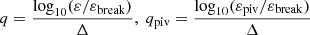
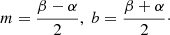
Two different approaches to measuring the width or sharpness of GRB data were undertaken by Axelsson & Borgonovo (2015) and Yu et al. (2015). Following Beloborodov (2013), Axelsson & Borgonovo (2015) define the width as the logarithmic ratio of the energies at the full width half maximum (FWHM) spectra:
and Yu et al. (2015) defined a sharpness angle (θ) at the νFν peak between two normalized fluxes at their respective normalized energies. With these definitions, both works define limits of different emission mechanisms in their respective measurement spaces as shown in Table 1. These mechanisms include a Planck function, single-particle synchrotron (SPS), synchrotron from a Maxwellian distribution of electrons (MS), and synchrotron from a power law distribution of electrons (PLS) with electron indices of either p = 2 or p = 4. In each approach, it was found that a majority of the data cannot be explained by synchrotron emission.
Derived physical widths.
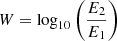
The sample selection in Axelsson & Borgonovo (2015) included GRBs from the Gamma-ray Burst Monitor (GBM) onboard the Fermi Gamma-ray Space Telescope (Meegan et al. 2009). The authors used all Band fits from the GBM catalog peak-flux spectral catalog regardless of which photon model best-fit the spectrum or if the Band function resulted in a failed maximum-likelihood fit. A cut was applied to the data requiring the low- and high-energy power laws of the Band function (α and β respectively) be α > −1.9 and β < −2.1. Herein, this analysis is replicated and then a further cut requiring that the best fitting spectrum as determined in the catalog be either the Band function or a smoothly-broken power law (SBPL) is applied. This eliminates spectra that may include Band parameters from failed fits due to a simpler function such as the exponentially-cutoff power law (CPL) or power law (PL) having been recorded as the best-fit. The width and the sharpness angle are computed from each observation in both the full and best-fit samples. The software used to compute the width and sharpness angle is released for the purpose of replication1.
Figure 1 shows that that when the cuts for best-fit spectrum are applied, the distributions shift to broader spectra or away from thermal spectra and towards optically-thin synchrotron spectra. Goldstein et al. (2012) note that with increasing signal-to-noise in the peak-flux spectra, the photon models shift from simple models such as the PL and CPL to more complex models such as the Band function or SBPL. This tentatively indicates that spectra are best fit by these simpler functions due to lack of photon statistics and not due to intrinsic physical reasons. The simpler functions are intrinsically narrower than the Band function and SBPL. Therefore, including spectra that were best fit by simpler (narrower) functions and not the Band function in the sample artificially leads to a bias towards narrower spectra. It is noted that Yu et al. (2015) computed the spectral sharpness on time-resolved spectra using the best-fitting model of each observed spectrum of the GBM time-resolved catalog (Yu et al. 2016).
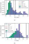 |
Fig. 1. Distributions of W (top) and θ (bottom) for the entire sample and the best-fit sample. |
The two width measures differ in their prediction for what types of spectra are viable. Figure 2 gives a toy example of how the measures look in νFν-space. Examining the W − θ plane, Figure 3 shows the full sample against the GBM best-fit sample as well as the regions allowed for different models. Over-plotted are the relation between W and θ with β = −2.25 and α ∈ { − 1.5, 0} as well as α = −0.8 and β ∈ { − 2.25, −4}. Interestingly, the best-fit sample follows a different trend than the full sample corresponding to the fixed-α curve. There is also a tentative correspondence of α and width with softer α values corresponding to larger width. It is clear that when a cut is not applied to the catalog fits to ensure that no failed fits are included, the width measures move away from the a clustering at “non-synchrotron” allowed values. Nevertheless, as pointed out in each work, the standard synchrotron models are strongly rejected by the width measures.
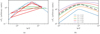 |
Fig. 2. Left: illustration of how W (green lines) and θ (via the red triangles) are realized on two different toy Band functions. Right: example of how the SBPL varies with Δ. For comparison, a Band function is superimposed in black dashed lines. |
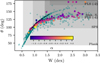 |
Fig. 3. W − θ plane from the full GBM catalog (teal) and the subsample of GRBs best fit by the Band function or a SBPL (purple-yellow). The boxes are the allowed regions for the corresponding physical emission mechanisms. The color of the subsample corresponds to the low-energy index (α) of the spectral fit. The two black dashed lines demonstrate how the W − θ plain evolves for fixed β (big dashes) and fixed α (small dashes). |
3. Synchrotron emission
Instead of employing empirical measures to infer if synchrotron can fit the data, let us now fit the data with a synchrotron model. A power law synchrotron model has been implemented into 3ML via astromodels2 following the method of Burgess et al. (2014) and described in Appendix A except that the Maxwellian part of the electron distribution is not included. In the spirit of open software, the model is made publicly available for use with 3ML3. The model has three free parameters: a normalization, the electron spectral index, and an energy scaling parameter (the magnetic field strength) proportional to the peak of the νFν spectrum. While it is numerically expensive to compute, it is functionally less complex than the four parameter Band function and five parameter SBPL thus making it less flexible.
3.1. Sample selection
The GBM has observed over 2000 GRBs with cataloged spectral parameters readily available online4. However, we must re-fit these data for this work. All spectral data used consist of 128 channel, time-tagged event (TTE) data obtained from the Fermi Science Support Center (FSSC). GRBs with cataloged parameters that were detected before 2017 and with best-fit peak-flux spectra of either Band or SBPL are used. These criteria result in a sample of 91 GRBs. Some catalog entries in the FSSC database had invalid response matrices and were discarded from the sample as it is important to use the exact responses that were used to compute the cataloged spectra5. Next, a cut on significance over background of 30σ was introduced to have a bright sample. A requirement that at least two Sodium Iodide (NaI) detectors in addition to one Bismuth Germinate (BGO) detector have acceptable viewing geometry of the GRB as denoted in the catalog further reduces the sample size. No selection on previously fitted spectral parameters was made to eliminate biasing the sample. Additionally, GRBs with Fermi Large Area Telescope (LAT) data are cut as they may include additional spectral features such as high-energy cutoffs. The final selections resulted in a sample of 44 GRBs.
Using the information provided in the GBM catalog, detectors, background and peak-flux intervals are selected to appropriately match with the selections used to produce the catalog. It was required that some background selections be modified as the ones specified in the online catalog occasionally contained on-source intervals. With these selections, the backgrounds were fitted with a series of polynomials of varying order via an unbinned Poisson likelihood and the best one was chosen via a likelihood ratio test (LRT). The modeled background count estimation and Gaussian error were extrapolated into the source interval as described in Greiner et al. (2016). For source intervals, the 1.024 s peak-flux intervals denoted in the catalog were selected to minimize the effects of spectral evolution as well as to keep the properties of the sample close to those which were used in Sect. 2.
3.2. Spectral fitting procedure
For spectral analysis, the Multi-Mission Maximum Likelihood framework6 (3ML Vianello et al. 2015) is used. The likelihood for the data is a Poisson-Gaussian likelihood to account for the Poisson nature of the total counts and the Gaussian nature of the modeled background (Arnaud 1996). 3ML allows for both maximum likelihood (MLE) and Bayesian posterior simulation (BPS) via a variety of optimization or sampling algorithms. For this study, BPS was chosen via the emcee (Foreman-Mackey et al. 2013) algorithm to fit the data in the sample. The fitting procedure involves two steps. First, MLE is used to find a starting point for the BPS. For MLE, the MINUIT (James & Roos 1975) optimization algorithm is used. With the MLE starting point, the posterior is sampled using flat, uninformative priors on all parameters7 To account for systematics in the GBM response matrices, the total effective area of all detectors is scaled to the brightest NaI detector by multiplicative constants. Instead of uninformative priors, informative Cauchy priors centered at unity, i.e., no correction, and width set to reflect the assumed 10% systematics in the GBM responses (Bissaldi et al. 2009) are used. The use of a Cauchy prior rather than a Gaussian is due to its wider shape around the mean reflecting the lack of knowledge about the systematics within 10%, but the belief that they are not too extreme.
Model comparison between the empirical functions used in Sect. 4 and synchrotron is not attempted because an empirical function can always be designed to fit the data with more predictability than a physical model. Moreover, it is invalid to treat the Band function as a null hypothesis against synchrotron emission as it is not a hypothesis, a special case of synchrotron (a so-called nested model), or part of a closed set of models which are known to include the true data-generating process8. In fact, this is the goal of empirical models. Instead, model checking of the synchrotron fits is performed via posterior predictive checks (PPC) which allows us to see if the observed data look plausible under the posterior predictive distribution. The details of the procedure are discussed in Appendix D.
3.3. Synchrotron results
In order to directly compare a success fit of the synchrotron model to the inference of the width measure, all data were also fitted by the Band function allowing for the Band derived width to be computed. This allows the fits to synchrotron to be displayed in the W − θ plane with their PPC values in Fig. 4a. Both width measures are computed from the Band function fit of the data. There are some spectra that lie in the excluded regions that have extremely poor PPC values as indicated by the blue X’s; however, several fits lie in the excluded region that can be well described by synchrotron. We demonstrate two of these fits in Fig. 5 which had similar PPC values as those fitted with the Band function. This explicitly demonstrates that models with very different shapes in photon space can be statistically similar in detector count space thus making empirically derived model assessment procedures very uninformative. Similar results were recently shown in Vianello et al. (2018). This is likely due to the Band function not properly modeling the inherent shape of the data and hence resulting in an misleading W or θ value. Therefore, empirical width measures fail to accurately predict if synchrotron is a viable spectral model for the data and hence cannot be used with the purpose for which they were designed. Synchrotron fit parameters are displayed in Appendix B. Figure 6 shows fits to both synchrotron and the Band function where the PPC for synchrotron was very bad and for the Band function acceptable. The pattern in the residuals for the synchrotron fit is not dissimilar to that of Fig. 5a. Naively, this would indicate that both fits should have bad PPCs. This is precisely why visual inspection of residuals which measures only a single point in the posterior can be misleading. PPCs have the advantage of measuring the deviation from the data across the entire posterior.
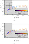 |
Fig. 4. W − θ plane with synchrotron PPCs (top) and Band PPCs (bottom). Blue X’s indicate extreme poor fits and color indicate deviation from 0.5, i.e., darker colors indicate better fits. The grey shaded regions are regions that would be excluded by synchrotron for an electron distribution of p = −4. |
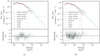 |
Fig. 5. Folded count spectra of two synchrotron fits (GRB 100131730 (left) and GRB 160101030 (right)) that had acceptable PPCs but would have been rejected via spectral width and sharpness angle as indicated in Fig. 4. The solid lines are the folded model through each GBM detector in the fit while the grey points indicate the raw count data. |
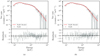 |
Fig. 6. Fit of synchrotron (left) and Band (right) to one of the detectors from GRB 160521385. Here, the PPC tail probability indicates that the synchrotron fit is very poor while the Band function accurately fits the data. A pattern can be seen in the residuals of the synchrotron fit. |
Goodness of fit via any method should be regarded with caution because one never has access to the true model. Moreover, it is preferable to compare physically motivated models to each other and chose the one which provides the best predictability of the data similar to what we have done with the empirical models. Nevertheless, PPCs for the Band function fits are computed and displayed in Fig. 4b. We can see that many of the Band function fits also do not accurately model the data according to the chosen PPC criterion, though the number of poor Band fits was smaller than poor synchrotron fits. The poor Band fits can be due to any number of issues such as unmodeled detector systematics like the K-edge non-linearity at ∼32 keV (Bissaldi et al. 2009; Goldstein et al. 2012). Therefore, I conclude that while synchrotron nor the Band function provide universally adequate fits, synchrotron does fit some spectra which would be ruled out by the width measures.
4. Fitting for the width
It is important to understand why the previous empirical width measures too conservatively reject synchrotron emission as shown in Sect. 3.3. Thus, the data are fitted with an SBPL of the form:
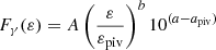
where
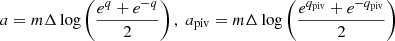
Here, εbreak is the break energy in keV, εpiv is the pivot energy, α and β are the low- and high-energy spectral indices respectively, and Δ is the break scale in decades of energy (for a similar use of a SBPL, see Ryde 1999). The proxy for the width of the spectral data will be Δ as it is a measure that is optimized during the fitting process and thus contains information about the width of the folded data. Figure 2 demonstrates how the function changes as a function of Δ for a range covering the distribution found from fitting the data. The intent of this fitting is not to introduce a new measure of width in the literature, but rather to see if the Band function is adequately modeling all features present in the data.
4.1. Fit results and model selection
Every GRB spectrum is fit to both the SBPL and Band function so that a comparison between the models can be made. The complexity of the SBPL function can result in local minima regardless of the optimization scheme; therefore, optimizing on a logarithmic grid of Δ and spectral normalizations results in a more robust result. Figure 7 illustrates the results of the fits to the two different functions. It can be seen that the SBPL allows for more posterior variance below the νFν peak due to its freedom to vary its width during the fit. Model selection via the likelihood ratio test (LRT) between the Band function an SBPL is not possible due to the fact that they are not nested functions. Additionally, for the empirical functions used, the aim is to assess whether a richer model is required to describe the data. The deviance information criteria (DIC) can be used to judge which model provides the best predictability of the data (see Appendix C). Table 2 details the results of the fits. Of the spectra fit, all but one are best described by the SBPL, i.e., positive δDIC in Table 2.
 |
Fig. 7. νFν spectra and 1σ contours of the SBPL (left) and Band (right) fits. The color corresponds to the 10 keV–4 MeV integrated energy flux (FE). The SBPL fits result in broader or smoother curvature around the νFν peak. |
Spectral fitting results.
The ability to fit a width parameter in the data indicates that the spectra have a variety of inherent widths rather than a single natural width of the Band function. Any change in the empirically measured width of the Band function is related to a change in spectral indices only. This variety is not captured by the Band function and hence, widths derived from the Band function can be systematically biased. It is noted that in GBM spectral catalogs, an SBPL is also fit to the spectra but its Δ is always fixed to 0.3 for historical reasons related to the bandpass of BATSE (Kaneko et al. 2006).
Another interesting feature of the SBPL fits is the different values of the measured α values. The distribution of α from the SBPL is shifted to softer values with a tail extending to hard values (see Fig. 8). Noticeably larger uncertainty on SBPL α’s is due to the additional freedom in the curvature. Physical inferences coming from empirical models are dependent on the spectral shape from which they are derived. The long standing paradigm that the Band function’s α should be used to infer physical spectra as well as the newly proposed limits of width measures do not hold if the Band function is not the best-fit to the data.
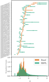 |
Fig. 8. Distributions of the low-energy index (α) from the Band and SBPL fits. The error bars represent the 0.68 highest posterior density intervals. There are systematic differences between the values of α due to the free curvature of the SBPL. The lower histograms are produced from the combined marginal distributions of the fits to fully incorporate the uncertainty in the fits. |
4.2. The smoothly-broken power law and synchrotron
Let us now examine the proxy for the width in the data, Δ, and its relation to synchrotron emission. To incorporate the uncertainty on Δ into the full sample distribution, the full marginal distributions from all fits are combined into a single distribution in Fig. 9. The distribution is unimodal with a tail extending to narrow widths. Hints of substructure are visually apparent in the distribution, but are likely an artifact of small sample size.
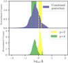 |
Fig. 9. Distribution of Δ from the fitted GRB spectra (top). Uncertainty on Δ is included via the marginal posteriors of each fit. Lower panel: marginal distributions of Δ for simulated synchrotron spectra with p = 2, 4. The 68% credible regions for these fits are superimposed on the full distribution. This demonstrates that the theoretical widths from pure synchrotron emission are consistent with the widths derived from the sample. |
A simple power law synchrotron model from Baring & Braby (2004), Burgess et al. (2014) was used to create synthetic count spectra using the GBM response matrices from a GRB in the sample. These synthetic spectra were then fit via BPS to a SBPL to estimate the values of Δ for different electron power law distributions. However, several factors influence the value of Δ beyond the shape of the electron distribution alone; most notably, the number of counts at high-energy in the synthetic spectra. This makes it difficult to set a hard limit on which values of Δ correspond to various synchrotron scenarios9. Nevertheless, examining the distribution of Δ expected from synchrotron with electron power law indices p = 2, 4 is necessary to follow the previous investigations into the spectral width. These limits are displayed in Fig. 9 both as the full marginal distribution from the BPS and as their respective 0.68 credible regions. The peak of the observed Δ distribution coincides with the SBPL-fitted Δ’s of the synthetic synchrotron spectra when p = 4. Thus, the distribution of widths from real data are marginally consistent with the limits derived from pure synchrotron emission. This is notably in contrast to the conclusions derived in previous studies providing further evidence that the natural width of the (less predictive) Band function is biasing the previously derived widths.
While these results are promising for synchrotron emission, it is worth examining their weaknesses. The difficulties of reconciling empirical models with physical spectra presents us with problems even when the more flexible SBPL is used to fit and characterize the spectra. Consider Fig. 10 which shows the fitted Band and SBPL functions to simulated synchrotron spectra. In the first case (Fig. 10a) the SBPL accurately models the spectra, in the second case (Fig. 10b) the SBPL overestimates the peak energy of the synthetic model and poorly models the non power law behavior of spectrum at low energies. In each case, the Band function fails to accurately model the synthetic spectrum. For these reasons, even though Δ serves as a better proxy for the width due to its ability to model the width directly in the data, it should not be used to set quantitative limits or inferences for the true underlying emission mechanisms in the data.
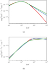 |
Fig. 10. Two examples of how the SBPL (blue) and Band (red) function fit a synthetic synchrotron spectrum (green). Top: an example where the SBPL models the synchrotron (W = −1.4, θ = 128) emission adequately while the Band function is too narrow and artificially softens β to compensate. Bottom: both the SBPL and Band functions are poor approximations of the true synchrotron spectrum (W = −1.6, θ = 170) and hence would result in poor empirical inference about the true underlying mechanism. |
5. Discussion
It has been demonstrated that the empirical width measures derived in Axelsson & Borgonovo (2015) and Yu et al. (2015) fail to predict when GRB data cannot be fit with a synchrotron spectra. Many of the spectra could be adequately fit with this model in regardless of the value of the spectral width derived from the Band function. These measures are derived from an empirical models that can poorly represent synchrotron emission. This was previously highlighted in Lloyd & Petrosian (2000) where parameterized synchrotron models were fit directly to the data and their asymptotic low-energy power law behavior was compared to that of the Band function. Only a small subset of GBM peak-flux spectra were examined and hence no physical conclusions about the validity of the synchrotron model used herein can be drawn. Such conclusions require examining the time-resolved spectra of individual GRBs. Instead, it was assessed whether empirical width measures which would have rejected synchrotron failed when synchrotron was actually fit to the same spectra. Furthermore, the question of whether synchrotron emission can be rejected when compared to other physical models has not been posed in this work as there are no other publicly available physical models to compare against. In reality, an emission model like synchrotron possesses multiple widths which may change non-linearly with the model parameters. This further exaggerates the issues with using secondary inference methods in fitted model space. This was not addressed directly in this study because the fact that the width fails to accurately predict the underlying model in the simple case is enough to demonstrate that fitting physical spectra is the proper way forward in GRB emission studies.
In an attempt to understand the spectral width by including the width of the data rather than the unfolded model, a sample of GRBs was re-fit with a SBPL and the distribution of its break scale parameter (Δ) was examined. With this measure, GRBs exhibit a variety of inherent data widths and the majority of these widths are not inconsistent with synchrotron emission. While this approach is a more appropriate empirical measure of the spectral width, it too suffers from the problem that the SBPL does not always model the shape of synchrotron emission properly. It is not entirely surprising that these empirical measures do not serve as quantitative inferences for physical models. Burgess et al. (2014, 2015) showed that synchrotron emission can fit GRBs that violate the “line-of-death” and that Band α values provide little insight into the presence of blackbodies in GRB spectra. Thus, it is strongly suggested that the fitting of physical models be performed to ascertain which model best represents the data.
While model checking can provide a qualitative guide to the validity of a spectra fit, other information should be used to fully justify the use of a model. These information can include physically motivated priors and predictions from time-evolving models such as those used in Dermer et al. (1999), Pe’er (2008), Bošnjak & Daigne (2014). For example, Burgess et al. (2016) used temporal predictions from Dermer et al. (1999) combined with synchrotron spectral fits to argue for an external shock interpretation of GRB 141028A. Therefore, without temporal or other information, it is important to not stress the physical implications of this work. Empirical models provide no such insight to physics other than assessing general features about the data e.g., the total flux, peak νFν energy and the existence of high-energy power laws. Deeper physical inferences from these empirical models should be regarded with caution until verified by complimentary analysis with physical emission models.
6. Supporting material
All processed GBM data files for use with XSPEC or 3ML as well as the analysis files containing the parameter marginals (readable by 3ML) are released for the purposes of replication. In addition, sample code for constructing the models used is also released10.
This is known as the ℳ-closed model comparison scenario (Vehtari & Ojanen 2012) under which LRTs and Bayes factors are a valid statistical test. This is explicitly not the case herein.
Both Axelsson & Borgonovo (2015) and Yu et al. (2015) calculate their respective limits in photon space rather than count space. Both works use Monte Carlo methods to calculate reportedly small errors on their respective measures.
All files can be located here: https://dataverse.harvard.edu/dataset.xhtml?persistentId=doi:10.7910/DVN/BDC2GS
Acknowledgments
I gratefully acknowledge fruitful discussion with Damien Bégué, Giacomo Vianello, David Yu, Patricia Schady, and Thomas Krühler concerning various aspects of this work.
References
- Ahlgren, B., Larsson, J., Nymark, T., Ryde, F., & Pe’er, A. 2015, MNRAS, 454, L31 [NASA ADS] [CrossRef] [Google Scholar]
- Akaike, H. 1977, Ann. Inst. Stat. Math., 29, 9 [CrossRef] [Google Scholar]
- Algeri, S., Conrad, J., & van Dyk, D. A. 2016, MNRAS, 458, L84 [NASA ADS] [CrossRef] [Google Scholar]
- Arnaud, K. A. 1996, Astron. Data Anal. Soft. Syst. V, 101, 17 [Google Scholar]
- Axelsson, M., & Borgonovo, L. 2015, MNRAS, 447, 3150 [NASA ADS] [CrossRef] [Google Scholar]
- Band, D., Matteson, J., & Ford, L. 1993, ApJ, 413, 281 [NASA ADS] [CrossRef] [Google Scholar]
- Baring, M. G. 2006, Adv. Space Res., 38, 1281 [NASA ADS] [CrossRef] [Google Scholar]
- Baring, M. G., & Braby, M. L. 2004, ApJ, 613, 460 [NASA ADS] [CrossRef] [Google Scholar]
- Beloborodov, A. M. 2013, ApJ, 764, 157 [NASA ADS] [CrossRef] [Google Scholar]
- Beniamini, P., & Piran, T. 2013, ApJ, 769, 69 [NASA ADS] [CrossRef] [Google Scholar]
- Bharali, P., Sahayanathan, S., Misra, R., & Boruah, K. 2017, New Astron., 55, 22 [NASA ADS] [CrossRef] [Google Scholar]
- Bissaldi, E., von Kienlin, A., Lichti, G., et al. 2009, Exp. Astron., 24, 47 [NASA ADS] [CrossRef] [Google Scholar]
- Blumenthal, G. R., & Gould, R. J. 1970, Rev. Mod. Phys., 42, 237 [NASA ADS] [CrossRef] [Google Scholar]
- Bošnjak, Ž., & Daigne, F. 2014, A&A, 568, A45 [NASA ADS] [CrossRef] [EDP Sciences] [Google Scholar]
- Briggs, M. S., Band, D. L., Kippen, R. M., et al. 1999, ApJ, 524, 82 [NASA ADS] [CrossRef] [Google Scholar]
- Buchner, J., Georgakakis, A., Nandra, K., & Hsu, L. 2014, A&A, 564, A125 [NASA ADS] [CrossRef] [EDP Sciences] [Google Scholar]
- Burgess, J. M., Preece, R. D., Connaughton, V., et al. 2014, ApJ, 784, 17 [NASA ADS] [CrossRef] [Google Scholar]
- Burgess, J. M., Ryde, F., & Yu, H.-F. 2015, MNRAS, 451, 1511 [NASA ADS] [CrossRef] [Google Scholar]
- Burgess, J. M., Bégué, D., Ryde, F., Omodei, N., Pe’er, A., & Racusin, J. 2016, ApJ, 822, 63 [NASA ADS] [CrossRef] [Google Scholar]
- Crider, A., Liang, E. P., Smith, I. A., & Preece, R. D. 1997, ApJ, 479, L39 [NASA ADS] [CrossRef] [Google Scholar]
- Dermer, C. D., Chiang, J., & Böttcher, M. 1999, ApJ, 513, 656 [NASA ADS] [CrossRef] [Google Scholar]
- Foreman-Mackey, D., Hogg, D. W., Lang, D., & Goodman, J. 2013, PASP, 125, 306 [CrossRef] [Google Scholar]
- Gelman, A. 2013, EJS, 7, 2595 [Google Scholar]
- Gelman, A., Hwang, J., & Vehtari, A. 2014, Stat. Comput., 24, 997 [CrossRef] [Google Scholar]
- Goldstein, A., Burgess, M. J., Preece, R. D., et al. 2012, ApJS, 199, 19 [NASA ADS] [CrossRef] [Google Scholar]
- Greiner, J., Sommer, M., Bade, N., et al. 1995, A&A, 302, 121 [NASA ADS] [Google Scholar]
- Greiner, J., Burgess, J. M., Savchenko, V., & Yu, H. F. 2016, ApJ, 827, L38 [NASA ADS] [CrossRef] [Google Scholar]
- Gruber, D., Goldstein, A., von Weller, A., et al. 2014, ApJS, 211, 12 [NASA ADS] [CrossRef] [Google Scholar]
- Iyyani, S., Ryde, F., Ahlgren, B., et al. 2015, MNRAS, 450, 1651 [NASA ADS] [CrossRef] [Google Scholar]
- Iyyani, S., Ryde, F., Burgess, J. M., Pe’er, A., & Bégué, D. 2016, MNRAS, 456, 2157 [NASA ADS] [CrossRef] [Google Scholar]
- James, F., & Roos, M. 1975, Comput. Phys. Commun., 10, 343 [NASA ADS] [CrossRef] [PubMed] [Google Scholar]
- Kaneko, Y., Preece, R. D., Briggs, M. S., et al. 2006, ApJS, 166, 298 [NASA ADS] [CrossRef] [Google Scholar]
- Lloyd, N. M., & Petrosian, V. 2000, ApJ, 543, 722 [NASA ADS] [CrossRef] [Google Scholar]
- Meegan, C., Lichti, G., Bhat, P. N., et al. 2009, ApJ, 702, 791 [NASA ADS] [CrossRef] [Google Scholar]
- Pe’er, A. 2008, ApJ, 682, 463 [NASA ADS] [CrossRef] [Google Scholar]
- Preece, R. D., Briggs, M. S., Mallozzi, R. S., et al. 1998, ApJ, 506, L23 [NASA ADS] [CrossRef] [Google Scholar]
- Protassov, R., van Dyk, D. A., Connors, A., Kashyap, V. L., & Siemiginowska, A. 2002, ApJ, 571, 545 [NASA ADS] [CrossRef] [Google Scholar]
- Ryde, F. 1999, Astrophys. Lett. Comm., 39, 281 [NASA ADS] [Google Scholar]
- Sari, R., Piran, T., & Narayan, R. 1998, ApJ, 497, L17 [NASA ADS] [CrossRef] [Google Scholar]
- Spiegelhalter, D. J., Best, N. G., Carlin, B. P., & Van Der Linde, A. 2002, J. R. Stat. Soc. Ser. B Stat. Methodol., 64, 583 [Google Scholar]
- Uhm, Z. L., & Zhang, B. 2014, Nature, 10, 351 [Google Scholar]
- van Dyk, D. A., & Kang, H. 2004, Stat. Sci., 19, 275 [CrossRef] [Google Scholar]
- Vehtari, A., & Ojanen, J. 2012, Stat. Surv., 6, 142 [CrossRef] [Google Scholar]
- Vianello, G., Lauer, R. J., Younk, P., et al. 2015, ArXiv e-prints [arXiv:1507.08343] [Google Scholar]
- Vianello, G., Gill, R., Granot, J., et al. 2018, ApJ, 864, 163 [NASA ADS] [CrossRef] [Google Scholar]
- Vurm, I., & Beloborodov, A. M. 2016, ApJ, 831, 175 [NASA ADS] [CrossRef] [Google Scholar]
- Wilks, S. S. 1938, Ann. Math. Stat., 9, 60 [Google Scholar]
- Yu, H.-F., van Eerten, H. J., Greiner, J., et al. 2015, A&A, 583, A129 [NASA ADS] [CrossRef] [EDP Sciences] [Google Scholar]
- Yu, H. F., Preece, R. D., Greiner, J., et al. 2016, A&A, 588, A135 [NASA ADS] [CrossRef] [EDP Sciences] [Google Scholar]
- Zhang, B.-B., Zhang, B., Liang, E.-W., et al. 2011, ApJ, 730, 141 [NASA ADS] [CrossRef] [Google Scholar]
- Zhang, B. B., Uhm, L. Z., Connaughton, V., et al. 2016, ApJ, 816, 72 [NASA ADS] [CrossRef] [Google Scholar]
Appendix A: Synchrotron modeling
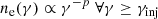
In order to fit synchrotron emission directly to the data, we assume a simple and pragmatic parameterization. More importantly, we assume the parameterization which captures the assumptions used to derive the rejection criteria for the various width measures adopted in previous works. The observed emission is assumed to come from a power law distribution of electrons that have been accelerated by an unspecified mechanism. Thus,
where γ is dimensionless electron energy, γinj the energy at which electrons are injected with spectral index p. The electrons are assumed to not cool via their radiation of synchrotron photons within a dynamical time. Therefore, we simply compute the synchrotron emission of this power law distribution by convolving it with the standard synchrotron emission kernel (Blumenthal & Gould 1970). Therefore,

where
and
Here, N is an arbitrary spectral normalization constant, B is the magnetic field strength, Bcrit = 4 × 10¹⁴ G, and γmax is the maximum electron energy which is set to have the spectral cutoff of the photon model above the GBM energy range.
With this simple parameterization, B and γinj are multiplicatively degenerate in setting the νFν peak of the spectrum, thus, the choice is made to fix γinj = 105 which is an arbitrary choice. This implies that the value of B found during fits is scaled and cannot be interpreted physically other than setting the location of the νFν peak. Therefore, there are three fitting parameters: B, p, and the arbitrary spectral normalization N. The high-energy shape of the photon spectrum is set by p while the low-energy shape is that of the synchrotron kernel. Note that this is the same functional form of synchrotron that is used to derive the conditions for rejecting synchrotron emission via the width or the line of death.
Appendix B: Synchrotron fit parameters
Here I include parameter plots for the synchrotron fits for reference. The synchrotron model in this work contains only two shape parameters and a normalization. Figure B.1 display the magnetic field strength and power law electron injection index from the fits. The plots are ranked and display the 68% highest density posterior intervals obtained from the fit. The electron spectral index is often found to be quite steep. This is not in conflict with expectations from relativistic, oblique shock acceleration theory (Baring 2006).
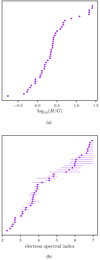 |
Fig. B.1. Parameter distributions of B and p from the synchrotron fits along with their 68% credible regions. |
It is stressed that the value of the magnetic field strength value has no scale unless assumptions about the emission region (emission radius, time scale, etc.) are assumed as noted in Appenidx A. For further discussion see Burgess et al. (2014).
Appendix C: Deviance information criteria
Model selection is one of the most difficult procedures in spectral analysis. The use of reduced χ2 as a model rejection criterion is not applicable to photon counting problems though it has previously been employed in GBM spectral catalogs. The lack of Gaussian likelihoods, generally non-linear models, unattained asymptotics of Wilk’s theorem (Wilks 1938) and the generally non-nested models employed (Protassov et al. 2002) violate a host of regularity conditions required to apply simple hypothesis testing. Additionally, the effective number of free parameters in a model is not necessarily equal to the number of fitted functional parameters. Therefore, rather than likelihood ratio tests, information criteria which seek to quantify the predictive accuracy of a model can be more useful for the current situation (see however the technique of Algeri et al. 2016, for an approach to assessing non-nested likelihood ratio tests)11.
The Akaike information criteria (AIC; Akaike 1977) has recently become common in X-ray spectral analysis as a model comparison tool (Zhang et al. 2011; Buchner et al. 2014); however, it relies of point estimates, an assumption of large number statistics, and only penalizes model complexity by the number of free model parameters. The deviance information criteria (DIC), uses the posterior mean, rather than a point estimate and penalizes model complexity with the effective number of free parameters which are a function of both the data and the model (Spiegelhalter et al. 2002).

where y are the data,  is the posterior mean and peff is the effective number of free parameters. The effective number of free parameters is a function of both the model and the data and can be negative if the posterior mean is far from the mode (Gelman et al. 2014). This allows for a model and data sensitive measure of a model’s data predictability.
Appendix D: Posterior predictive checks
Assessment of a model’s fit to data via posterior predictive checks (PPCs) allows for incorporating information in the posterior into a quantitative goodness of fit measure for future observations. The usefulness of PPCs in X-ray spectral analysis has been demonstrated in van Dyk & Kang (2004). PPCs offer a guide to model assessment but are simply a self-consistency check. In the current situation we lack other physical models with which to check against. The posterior predictive distribution is defined as
where y are the data and yrep are data replicated from a the posterior and θ are the parameters. One way to assess the lack of fit of data to this distribution is a tail-area probability known as the posterior p-value:

Here, T is a test statistic. For this work, 500 replicated spectra are produced from the simulated posterior and T(y, θ) is defined as the likelihood value for the given parameter. We compare these test statistics to that of the actual data to arrive at a measure of goodness of fit. A fit that adequately models the data should have pB ∼ 0.5 (Gelman 2013). Thus, we define a so-called good fit as being |pB − 0.5|∼0.
Model assessment and comparison is an ongoing and active part of statistical research. Further details can be found in Vehtari & Ojanen (2012).
All Tables
All Figures
|
Fig. 1. Distributions of W (top) and θ (bottom) for the entire sample and the best-fit sample. |
| In the text | |
|
Fig. 2. Left: illustration of how W (green lines) and θ (via the red triangles) are realized on two different toy Band functions. Right: example of how the SBPL varies with Δ. For comparison, a Band function is superimposed in black dashed lines. |
| In the text | |
|
Fig. 3. W − θ plane from the full GBM catalog (teal) and the subsample of GRBs best fit by the Band function or a SBPL (purple-yellow). The boxes are the allowed regions for the corresponding physical emission mechanisms. The color of the subsample corresponds to the low-energy index (α) of the spectral fit. The two black dashed lines demonstrate how the W − θ plain evolves for fixed β (big dashes) and fixed α (small dashes). |
| In the text | |
|
Fig. 4. W − θ plane with synchrotron PPCs (top) and Band PPCs (bottom). Blue X’s indicate extreme poor fits and color indicate deviation from 0.5, i.e., darker colors indicate better fits. The grey shaded regions are regions that would be excluded by synchrotron for an electron distribution of p = −4. |
| In the text | |
|
Fig. 5. Folded count spectra of two synchrotron fits (GRB 100131730 (left) and GRB 160101030 (right)) that had acceptable PPCs but would have been rejected via spectral width and sharpness angle as indicated in Fig. 4. The solid lines are the folded model through each GBM detector in the fit while the grey points indicate the raw count data. |
| In the text | |
|
Fig. 6. Fit of synchrotron (left) and Band (right) to one of the detectors from GRB 160521385. Here, the PPC tail probability indicates that the synchrotron fit is very poor while the Band function accurately fits the data. A pattern can be seen in the residuals of the synchrotron fit. |
| In the text | |
|
Fig. 7. νFν spectra and 1σ contours of the SBPL (left) and Band (right) fits. The color corresponds to the 10 keV–4 MeV integrated energy flux (FE). The SBPL fits result in broader or smoother curvature around the νFν peak. |
| In the text | |
|
Fig. 8. Distributions of the low-energy index (α) from the Band and SBPL fits. The error bars represent the 0.68 highest posterior density intervals. There are systematic differences between the values of α due to the free curvature of the SBPL. The lower histograms are produced from the combined marginal distributions of the fits to fully incorporate the uncertainty in the fits. |
| In the text | |
|
Fig. 9. Distribution of Δ from the fitted GRB spectra (top). Uncertainty on Δ is included via the marginal posteriors of each fit. Lower panel: marginal distributions of Δ for simulated synchrotron spectra with p = 2, 4. The 68% credible regions for these fits are superimposed on the full distribution. This demonstrates that the theoretical widths from pure synchrotron emission are consistent with the widths derived from the sample. |
| In the text | |
|
Fig. 10. Two examples of how the SBPL (blue) and Band (red) function fit a synthetic synchrotron spectrum (green). Top: an example where the SBPL models the synchrotron (W = −1.4, θ = 128) emission adequately while the Band function is too narrow and artificially softens β to compensate. Bottom: both the SBPL and Band functions are poor approximations of the true synchrotron spectrum (W = −1.6, θ = 170) and hence would result in poor empirical inference about the true underlying mechanism. |
| In the text | |
|
Fig. B.1. Parameter distributions of B and p from the synchrotron fits along with their 68% credible regions. |
| In the text | |
Current usage metrics show cumulative count of Article Views (full-text article views including HTML views, PDF and ePub downloads, according to the available data) and Abstracts Views on Vision4Press platform.
Data correspond to usage on the plateform after 2015. The current usage metrics is available 48-96 hours after online publication and is updated daily on week days.
Initial download of the metrics may take a while.