| Issue |
A&A
Volume 628, August 2019
|
|
|---|---|---|
| Article Number | A127 | |
| Number of page(s) | 7 | |
| Section | Planets and planetary systems | |
| DOI | https://doi.org/10.1051/0004-6361/201935655 | |
| Published online | 20 August 2019 | |
Upper limits on the water vapour content of the β Pictoris debris disk★
1
Department of Astronomy, AlbaNova University Center, Stockholm University,
106 91 Stockholm, Sweden
e-mail: This email address is being protected from spambots. You need JavaScript enabled to view it.
; This email address is being protected from spambots. You need JavaScript enabled to view it.
; This email address is being protected from spambots. You need JavaScript enabled to view it.
2
Konkoly Observatory, Research Centre for Astronomy and Earth Sciences, Hungarian Academy of Sciences, Konkoly-Thege Miklós út 15–17,
1121 Budapest, Hungary
3
Subaru Telescope, National Astronomical Observatory of Japan,
650 North A’ohoku Place,
Hilo,
HI 96720, USA
4
Department of Astronomy and Astrophysics, University of Toronto,
Toronto,
ON M5S 3H4, Canada
5
Department of Space, Earth and Environment, Chalmers University of Technology, Onsala Space Observatory,
439 92 Onsala, Sweden
Received:
10
April
2019
Accepted:
23
June
2019
Abstract
Context. The debris disk surrounding β Pictoris has been observed with ALMA to contain a belt of CO gas with a distinct peak at ~85 au. This CO clump is thought to be the result of a region of enhanced density of solids that collide and release CO through vaporisation. The parent bodies are thought to be comparable to solar system comets, in which CO is trapped inside a water ice matrix.
Aims. Since H2O should be released along with CO, we aim to put an upper limit on the H2O gas mass in the disk of β Pictoris.
Methods. We used archival data from the Heterodyne Instrument for the Far-Infrared (HIFI) aboard the Herschel Space Observatory to study the ortho-H2O 110–101 emission line. The line is undetected. Using a python implementation of the radiative transfer code RADEX, we converted upper limits on the line flux to H2O gas masses. The resulting lower limits on the CO/H2O mass ratio are compared to the composition of solar system comets.
Results. Depending on the assumed gas spatial distribution, we find a 95% upper limit on the ortho-H2O line flux of 7.5 × 10⁻²⁰ W m−2 or 1.2 × 10⁻¹⁹ W m−2. These translate into an upper limit on the H2O mass of 7.4 × 10¹⁶–1.1 × 10¹⁸ kg depending on both the electron density and gas kinetic temperature. The range of derived gas-phase CO/H2O ratios is marginally consistent with low-ratio solar system comets.
Key words: stars: individual: β Pictoris / submillimeter: planetary systems / methods: observational / circumstellar matter
Herschel is an ESA space observatory with science instruments provided by European-led PI consortia and with important participation from NASA.
International Research Fellow of Japan Society for the Promotion of Science (Postdoctoral Fellowships for Research in Japan (Standard)).
© ESO 2019
1 Introduction
Circumstellar debris disks are made up of planetesimals and dust and can be thought of as the remnants of planet formation. The small dust grains in debris disks are continuously removed by radiation pressure on timescales that are short compared to the age of the system. Therefore, the dust must be secondary and is replenished through collisions between larger bodies (e.g., Wyatt 2008, 2018). Thus, there exists a direct connection between the observed dust and the building blocks of planets. The study of debris disks is part of our efforts to understand the formation and evolution of planetary systems.
For a small subset of debris disks, gas has been detected in addition to the dust. Thanks to sensitive observations of CO emission with the Atacama Large Millimeter/submillimeter Array (ALMA), the set of known gaseous debris disks was recently significantly expanded (e.g., Lieman-Sifry et al. 2016; Moór et al. 2017). Most of the approximately 20 gaseous debris disks we currently know are hosted by young A-type stars. In general, the origin of this gas remains unknown. It could be primordial (i.e., leftover from the protoplanetary phase) or, like the dust, secondary (i.e., released from volatile-rich, icy bodies). For a few systems (e.g., β Pictoris, see below), there is evidence for a secondary origin of the gas. Studying this secondary gas allows us to constrain the composition of the parent bodies and compare it to solar system comets (Xie et al. 2013; Kral et al. 2016; Marino et al. 2016; Matrà et al. 2017a,b, 2018).
One example of a gaseous debris disk is found around the A-type star β Pictoris. This system has been the subject of numerous studies over the last three decades, with the IRAS discovery of the infrared (IR) excess of its debris disk dating back to 1984 (Smith & Terrile 1984). It is nearby (19.75 pc, Gaia Collaboration 2018), young (23 ± 3 Myr, Mamajek & Bell 2014) and harbours a giant planet at ~10 au, discovered by direct imaging (Lagrange et al. 2009). The belt of parent bodies of the disk is located at around 100 au (Dent et al. 2014), and is edge-on, making it an ideal target for absorption spectroscopy. The system has served as a laboratory for the study of various processes in a newly formed planetary system.
Several atomic metal lines have been detected in the gas phase of the β Pic disk. The lines appear in both absorption against the star and in emission. Besides species such as Fe, Na, and Ca+ (Brandeker et al. 2004), this includes oxygen (Brandeker et al. 2016) as well as both neutral and ionised carbon (Roberge et al. 2006; Cataldi et al. 2014, 2018; Higuchi et al. 2017). Carbon monoxide is the only molecule detected so far (e.g., Liseau & Artymowicz 1998; Dent et al. 2014; Matrà et al. 2018). In addition, Wilson et al. (2019) recently detected N in absorption and Wilson et al. (2017) detected H in close vicinity to the star (i.e., not in the main gas/dust disk). Elemental abundances differ significantly from solar values. In particular, there is an overabundance of C (Roberge et al. 2006; Cataldi et al. 2014), and perhaps O (Brandeker et al. 2016), relative to other elements.
Different pieces of evidence suggest that the gas in the β Pic disk is secondary. Firstly, the spatial distributions of gas and dust are similar (e.g., Brandeker et al. 2004; Dent et al. 2014), consistent with a common origin, and secondly, the dynamical lifetime of the gas is short compared to the age of the system (Fernández et al. 2006). Additional evidence comes from CO. Matrà et al. (2017a) showed that there is not enough H2 in the disk to shield CO from photodissociation over the age of the system. The photodissociation lifetime of CO is only ~50 yr (Cataldi et al. 2018), implying a replenishment mechanism. Therefore, the CO is believed to be produced from volatile-rich cometary bodies. At least part of the observed C and O must therefore come from CO photodissociation.
The CO emission from the β Pic disk was first resolved by ALMA (Dent et al. 2014). The data revealed a surprising asymmetry: a CO clump on the southwest (SW) side of the disk at a radial distance of ~85 au. The clump is interpreted as a site of enhanced CO gas production caused by an enhanced collision rate among volatile-rich bodies. The suggested mechanisms for the enhanced collision rate are a yet unseen, outward-migrating planet capturing comets in a resonance trap (Matrà et al. 2017a); a previous giant collision (Jackson et al. 2014); or an eccentric disk produced from a tidal disruption event (Cataldi et al. 2018).
Solar system comets consist mainly of amorphous water ice in a matrix structure, wherein volatiles like CO become trapped (Whipple 1950). If the CO seen in the β Pic disk is indeed produced by colliding comet-like bodies, we would expect water vapour to be produced as well, for example by photosputtering of grains formed in a collisional cascade; see Sect. 5. Based on the excitation conditions of O I, Kral et al. (2016) indirectly constrained the H2O/CO ratio of the β Pic comets. They find a lower ratio than what is observed for solar system comets, suggesting that the comets in the β Pic disk are depleted in water. However, their assumed spatial distribution of the gas (accretion disk) turned out to be inconsistent with new observations (Cataldi et al. 2018). It is unclear how this impacts their estimated H2O/CO ratio.
Matrà et al. (2017a,b) and Marino et al. (2016) found that the CO+CO2 mass abundances of the comets in the β Pic, Fomalhaut, and HD 181327 disks are consistent with abundances measured in solar system comets. Using data from the Submillimeter Array (SMA), Matrà et al. (2018) showed that the comets in the β Pic disk have a HCN/(CO+CO2) ratio of outgassing rates that is consistent with but at the low end of what is observed for solar system comets. This might be caused by the outgassing mechanism, or it might indicate a true depletion of HCN with respect to solar system comets.
One motivation to study the water content of extrasolar planetesimals comes from an astrobiological perspective. Water is required for life as we know it. Most of the water on Earth may have been delivered by asteroids (e.g., Alexander et al. 2012), and similar processes might occur in extrasolar systems. In this work, we aim to further investigate the water content of the bodies in the β Pic disk with a more direct approach compared to the Kral et al. (2016) study. We use an archival non-detection from Herschel/HIFI of the rotational 110 –101 transition of o-H2O. Our paper is organised as follows: in Sect. 2, we describe our observations. We derive upper limits on the o-H2O 110 –101 flux and the H2O mass in Sect. 3, and report them in Sect. 4. In Sect. 5, we discuss what our measurements tell us about the water content of the bodies in the β Pic disk. We summarise our results in Sect. 6.
2 Observations and data reduction
The star β Pictoris was observed on July 19, 2010 (ID 1342200907), with the Heterodyne Instrument for the Far-Infrared (HIFI, de Graauw et al. 2010) aboard Herschel (Pilbratt et al. 2010), as a Guaranteed Time observation. The Single Point mode of the High Resolution Spectrometer was used, and the observation time was roughly 58 min. The lower sideband of band 1b was chosen in order to observe the o-H2O 110 –101 line, which has arest frame frequency of 556.936 GHz (National Institute of Standards and Technology, Physical Measurement Laboratory 2016). The spectral resolution was 125 kHz. The FWHM beam size was 37′′. The clump of CO is at a separation of 4.3′′ from the centre of the beam, meaning the beam sensitivity at its location was 96%. As the bulk of the CO as determined by Dent et al. (2014) is within this angular distance, we do not perform any beam sensitivity correction in the data analysis.
The data were first processed in the Herschel Interactive Processing Environment (HIPE version 13.0.0, Ott 2010). The antenna temperature was converted to a flux density by assuming a point source. Standing waves were removed and a baseline correction was carried out. The four sub-bands were stitched together and since the Frequency Shift mode was used, the spectra were folded. The H and V polarisations were then averaged over. The spacing of data points was 0.12 MHz, but to ensure there were no remaining standing waves to correlate adjacent flux points, we calculated the auto-correlation in the background region (see below) using the built-in correlate function of NumPy. The FWHM of the best-fit Gaussian of the correlation function was then taken to be the correlation length, and was 0.3631 MHz. The spectrum was then rebinned to 0.5 MHz to ensure the bins were independent of one another. Figure 1 shows the reduced spectrum in a velocity scale relative to the β Pic system, where the star has a heliocentric velocity of 20.5 km s−1 (Brandeker 2011).
3 Analysis
3.1 Upper limit on the o-H2O 110 –101 flux
We assume that H2O and CO are released at the same locations in the disk and subsequently photodissociated on short timescales compared to the orbital timescale. At 85 au, the CO lifetime is ~50 yr. The lifetime of H2O is even shorter: using the stellar spectrum supplemented with UV data described in Cataldi et al. (2018) and photodissociation cross sections from the Leiden Observatory database of the “photodissociation and photoionisation of astrophysically relevant molecules1 ” (Mordaunt et al. 1994; van Harrevelt & van Hemert 2008; Heays et al. 2017), we calculate a lifetime of 3.5 d under the assumption that water is not shielded from dissociating radiation. This assumption is justified since neither CO nor C can shield water, as their cross sections for dissociation and ionisation, respectively, do not substantially overlap in wavelength with the cross section for water dissociation. Furthermore, we verified that water self-shielding is irrelevant for the column densities considered here. This implies that, while the CO may have some time to orbitally evolve before being dissociated (the orbital period at 85 au is ~600 yr), any water vapour must be close to its point of release.
In one of the proposed CO-production scenarios, the production region is caused by debris in eccentric orbits converging at a fixed region in space corresponding to the southwestern CO-“clump”. Orbital motion then moves the gas out of this region forming a tail (Dent et al. 2014). Due to the shorter lifetime of H2O, no water vapour tail would be formed and all H2O is expected to be restricted to the clump region. In the other proposed scenario, the CO production region is due to a mean motion resonance with an inner planet, in which case the production region is more spread out (Matrà et al. 2017a). To accommodate both scenarios, we test for two extremes: firstly with the assumption that the bulk of the gas production takes place in the clump region, and secondly using the assumption that the CO distribution reflects the production region, in which case the H2O would share the spatial distribution of the CO.
The spectrum does not contain any clear emission line. To estimate a reliable upper limit of the line flux, a Monte Carlo approach is used. Onemillion noise realisations are made by scaling a vector of random numbers drawn from a standard normal distribution by the error σi of the flux density, estimated as the standard deviation of the background flux density, where the background region is taken to be v > −0.56 km s−1 or v < −6.2 km s−1. Each noise realisation is then separately added to the original spectrum to produce 106 spectra with different noise realisations. A line profile is then fit by a χ2 minimisation in each alternate spectrum to obtain a best-fit flux. As line profiles we use the ones corresponding to the two scenarios (Fig. 1): in the case of H2O located in a clump we assume a Gaussian blueshifted to −3.5 km s−1 with a full width at half maximum (FWHM) matching that of the CO, namely 1 km s−1 (Dent et al. 2014). For the case where H2O shares the spatial distribution of CO, we use the same spectral profile as found for CO 3–2 (Matrà et al. 2017a). Since the shapes of the profiles are kept fixed, the only free parameter is the integrated flux, which is allowed to take on negative values. In this way a Gaussian distribution of one million values of the integrated line flux for each case is computed, from which the 95% upper limits are derived.
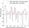 |
Fig. 1 95% upper limit models superimposed on the observed spectrum. The red solid line shows the expected profile coming from H2O restricted to the SW clump. The blue dashed line shows the profile from the model assuming the same spatial distribution for H2O as for CO (see Sect. 5). |
3.2 Upper limit on the H2O mass
To convert the upper limits on the line flux into upper limits on the H2O mass, we use pythonradex2, a Python implementation of the RADEX code (van der Tak et al. 2007). The program uses an escape probability formalism and an accelerated Lambda iteration (ALI) scheme to solve the radiative transfer in the non-local thermal equilibrium (non-LTE) regime, given the total gas mass, and the densities and kinetic temperature of the colliders. In this way we are able to calculate the expected line flux for a given ortho-H2O gas mass. To convert to total gas mass, a H2O ortho:para ratio of 3:1 is assumed.
The code assumes a uniform, spherical geometry (we choose a radius of 30 au) and that the line profile has a boxcar shape (we choose a width of 1.5 km s−1). Our model is thus not fully self-consistent, since we used different line profiles to compute upper limits on the line flux (Fig. 1). The assumption of a spherical rather than a flattened, edge-on distribution may be relevant if the emitting region is optically thick. We study this possibility in Sect. 5.
We assume that electrons are the only relevant colliders with H2O (e.g., Kral et al. 2016). While a certain amount of hydrogen should also be present (e.g., from H2O photodissociation), the collisional excitation rates with H are several orders of magnitude lower compared to electrons (A. Faure, priv. comm.). We use excitation rates from the LAMDA database3 (Schöier et al. 2005) published by Faure et al. (2004), supplemented at kinetic temperatures below 200 K with unpublished data (A. Faure, priv. comm.). In the low-temperature regime the data consist of excitation rates of transitions between the 14 lowest-lying levels of o-H2O, while the high-temperature regime includes 397 additional levels for a total of 411. The o-H2O 110 –101 emission line corresponds to the transition between the two lowest levels. We confirm that no levels other than the two lowest are significantly populated, which could otherwise lead to fluorescence effects. In any case, if fluorescence was important, neglecting it would result in an underestimate of the line flux from the transition and therefore an overestimated upper limit on the mass.
In addition to collisional excitation from electrons we also include a background radiation field consisting of the cosmic microwave background, stellar photons directly from β Pic, and a model of the dust radiation field. The latter is as shown in Fig. B1 of Kral et al. (2017) and represents the dust radiation field in the midplane of the disk at the position angle of the clump (L. Matrá, priv. comm.). The e− –H2O collisions are by far the most important excitation mechanism, hence including the background field does not change the results significantly.
Matrà et al. (2017a) studied the CO J = 3–2/J = 2–1 line ratio and found the gas kinetic temperature to be between 40 and a few hundred Kelvin, and the electron density in the disk to be around 102 –103 cm−3. The temperature and electron densities are degenerate with their estimates depending on the assumed mean molecular weight of the gas. We therefore consider four different temperatures (50, 100, 200 and 400 K) and three different electron densities (100, 300 and 900 cm−3). In addition, we also perform a calculation assuming LTE. For a given electron density and temperature, we then compute the o-H2O 110 –101 flux as a function of mass.
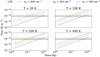 |
Fig. 2 Computed o-H2O 110 –101 flux as a function of H2O gas mass. Four different gas kinetic temperatures are shown; 50 K (top left), 100 K (top right), 200 K (bottom left) and 400 K (bottom right). Solid lines show LTE calculations, while each other line corresponds to an electron density; 100 (dashed), 300 (dotted), and 900 cm−3 (dash-dotted). The horizontal lines in each plot indicate the 95% line flux upper limit obtained from the data (Sect. 3.1). The solid horizontal line corresponds to using a Gaussian profile, and the dashed line to the spectral profile matching the CO. |
4 Results
The resulting upper limit on the o-H2O 110 –101 flux depends on the assumed line profile. With all water vapour constrained to the clump, the narrower spectral line results in a 95% upper limit of 7.5 × 10⁻²⁰ W m−2, while the corresponding limit for the broader spectral line coming from the spread-out scenario is 1.2 × 10⁻¹⁹ W m−2. Figure 1 shows a plot of the spectrum after the initial processing in HIPE with the spectral lines from both scenarios plotted at their 95% upper limit flux.
Figure 2 shows the calculated flux versus mass, as well as the observed line flux 95% upper limits, indicated by the horizontal lines. We take the intersection of these lines with the curves corresponding to different electron densities as our o-H2O gas mass upper limits. The measured CO mass of 2.0 × 10²⁰ kg (Matrà et al. 2017a) is then assumed in order to calculate (T, ne)-dependent lower limits on theCO/H2O, as presentedin Table 1. Finally, Table 2 shows the values of the optical depth at the centre of the emission line τν0, the line excitation temperatureTex, and the molecular column density  , all evaluated at the respective gas mass upper limits.
5 Discussion
A few different trends can be inferred from the plots in Fig. 2. The computed line flux generally increases with both gas mass and electron density, as one would expect. For a fixed line flux, the gas mass decreases as the electron density increases. In the presence of more electrons, the H2O molecules are excited more often, and therefore fewer of them are needed to account for the flux.
With increasing temperature, other behaviours become apparent. Firstly, the line flux in the LTE case decreases with increasing temperature. This is a result of higher levels becoming increasingly more excited than the ground level, decreasing the emission from the latter. Secondly, all curves flatten out at high masses. This is due to the emission becoming optically thick, and therefore more mass can be added without raising the flux. The effect is most pronounced for high densities.
The solid-phase number ratio 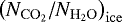 in solar system comets has been found to be between 0.002 and 0.23 (Bockelée-Morvan & Biver 2017). Taking into account the relative atomic weights and photodissociation lifetimes at 85 au in the β Pic system of the two species, the gas-phase mass ratio
 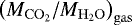 is determined as:
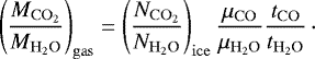 (1)
(1)
This corresponds to gas-phase mass ratios between roughly 16 and 1900, assuming continuous production.
Considering first the case of the narrow spectral line, the observed lower limits are compatible with solar system compositions for all cases of electron densities ne = 100, 300 cm−3. ALMA observations of CO lines find ne ~ 300 cm−3 at the location of the CO (Fig. 11 in Matrà et al. 2017a). None of the cases of ne = 900 or the T = 50, 100 K cases in LTE are compatible with solar system compositions, as the H2O content is too low. For the scenario of the broader spectral line, only the two LTE cases with T = 50, 100 K lie outside the expected range from solar system comets. As the gas is not expected to be in LTE, these two cases seem unlikely.
The true distribution of H2O probably lies somewhere between the two extremes we test for. It is difficult to say how likely each scenario is, and also whether or not the lower limits on the CO/H2O ratio will be pushed upwards by more sensitive observations. Because of the possibility of discrepancies between our derived values and solar system comet values, we here speculate on explanations for this.
One possible explanation could be episodic gas production; CO has a dissociative lifetime of ~50 yr, but H2O survives for only 3.5 days. If the gas is produced in intermittent bursts with a frequency lower than once every few days, rather than continuously, we may have caught the system at a time where H2O is gone but CO remains. In that case another observation made just days apart from this one could lead to very different results. Another possibility is that low-velocity collisions between the planetesimals can cause CO to vaporise while leaving the less-volatile H2O behind (Dent et al. 2014). However, since the collisions are continually taking place, the planetesimals will eventually be ground down to dust grains, from which the H2O is efficiently UV photo-sputtered by β Pic (Grigorieva et al. 2007). A third possibility is that the clump radius is significantly smaller than our assumed 30 au, in which case the increased optical depth would mean that more mass can be present without violating the upper limit on the flux, particularly so for low temperatures. We plot the inferred mass upper limit for the case of a narrow spectral line against emission region radius in Fig. 3. We see that the radius would have to shrink to less than about 15 au for the derived mass to change significantly. Finally, the non-detection of H2O could be caused by a different initial composition of the colliders compared to solar system comets. The β Pic system has been observed several times to have peculiar gas abundances. Carbon is particularly overabundant compared to Fe (Roberge et al. 2006; Brandeker 2011; Cataldi et al. 2018), and oxygen is likely overabundant as well (Brandeker et al. 2016). Integrating the spatial number density of Fe from Nilsson et al. (2012), we find the total Fe mass to be MFe = 3.0 × 10¹⁹ kg. Comparing to a possible mass range of C (MC = [3.0 − 18.5] × 1021 kg, Cataldi et al. 2018), a C/Fe number ratio of 50–330 times solar values is obtained. Given the different spatial distributions found for C and Fe, perhaps this is simply a reflection of different origins, where the C could be mostly produced by dissociation of CO and CO2. If so, the O abundance would likewise mostly be formed by dissociation of CO, CO2, and H2O, and an estimate of the O abundance could be used to indirectly constrain the H2O/CO ratio. Unfortunately, the O mass is difficult to derive since the detected O I 63 μm emission is optically thick and strongly dependent on the spatial distribution and excitation conditions. Other dissociation products that could be searched for are H and OH, both of which are accessible for sensitive measurements at radio frequencies by the planned Square Kilometer Array.
H2O gas mass 95% upper limits and corresponding CO/H2O lower limits.
Optical depth τν0, excitation temperature Tex, and H2O column density  .
.
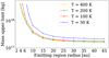 |
Fig. 3 Derived mass upper limits as a function of emission region radius (assumed to be spherical). In our calculations, we use a radius of 30 au. The mass upper limits are for the case of a Gaussian line profile. |
6 Summary
We present a HIFI non-detection of H2O emission in the β Pictoris system. We find the 95% upper limit on the o-H2O 110 –101 line flux to be 7.5 × 10⁻²⁰ W m−2 or 1.2 × 10⁻¹⁹ W m−2, depending on the assumed production region of H2O. We test for two scenarios: one where all H2O production occurs at the place of the previously observed CO clump, and one where the production follows the entire CO spatial profile.
Calculating the level populations for the case of an electron density of 300 cm−3, this is translated to an upper limit on the H2O gas mass of (1.75–3.96) × 1017 kg, depending on both the production region and the kinetic gas temperature, which has previously been constrained to be between 40 and a few hundred Kelvin (Matrà et al. 2017a).
From the mass upper limits we derive lower limits on the CO/H2O mass ratio. Assuming again ne ~ 300 cm−3, the ratios inthe scenario of a clump production region fall between 864 and 1140. For the spread-out production scenario, the ratios are between 505 and 681. Since the emission is thought to originate from colliding comet-like bodies, we can compare these lower limits to known solar system values of 16–1900 (Bockelée-Morvan & Biver 2017). In the case of this chosen electron density, the ratios fall within the solar system composition range. For electron densities of 900 cm−3 and the cases of LTE with T = 50, 100 K, all lower limits on CO/H2O in the clump production scenario are larger than expected from solar system values, indicating water-poor conditions. In the spread-out production scenario, this is only true for an emission region in LTE with temperatures of T = 50, 100 K. If the comets of β Pic are indeed water-poor, possible explanations are episodic gas production or simply an initial composition that is different from that of solarsystem comets.
Since the now decommissioned HIFI instrument was unique in targeting the H2O 110 –101 line, more sensitive measurements await future instrumentation. Measuring the dissociation products OH, H, or O could potentially indirectly constrain the water content of the colliding comets. The future Square Kilometer Array will be uniquely sensitive to both H and OH.
Acknowledgements
We thank Alexandre Faure for providing collisional excitation rates at low temperatures, and Luca Matrà for sharing the model of the dust radiation field and the ALMA data of CO. We also thank the referee for helpful and thorough comments. HIFI has been designed and built by a consortium of institutes and university departments from across Europe, Canada and the United States under the leadership of SRON Netherlands Institute for Space Research, Groningen, The Netherlands and with major contributions from Germany, France and the US. Consortium members are: Canada: CSA, U.Waterloo; France: CESR, LAB, LERMA, IRAM; Germany: KOSMA, MPIfR, MPS; Ireland, NUI Maynooth; Italy: ASI, IFSI-INAF, Osservatorio Astrofisico di Arcetri-INAF; Netherlands: SRON, TUD; Poland: CAMK, CBK; Spain: Observatorio Astronómico Nacional (IGN), Centro de Astrobiología (CSIC-INTA). Sweden: Chalmers University of Technology - MC2, RSS & GARD; Onsala Space Observatory; Swedish National Space Board, Stockholm University - Stockholm Observatory; Switzerland: ETH Zurich, FHNW; USA: Caltech, JPL, NHSC. This work was supported by the Momentum grant of the MTA CSFK Lendület Disk Research Group and by JSPS KAKENHI Grant Number JP16F16770. This research has made use of NASA’s Astrophysics Data System.
References
- Alexander, C. M. O., Bowden, R., Fogel, M. L., et al. 2012, Science, 337, 721 [NASA ADS] [CrossRef] [PubMed] [Google Scholar]
- Bockelée-Morvan, D., & Biver, N. 2017, Phil. Trans. R. Soc. London, Ser. A, 375, 20160252 [Google Scholar]
- Brandeker, A. 2011, ApJ, 729, 122 [NASA ADS] [CrossRef] [Google Scholar]
- Brandeker, A., Liseau, R., Olofsson, G., & Fridlund, M. 2004, A&A, 413, 681 [NASA ADS] [CrossRef] [EDP Sciences] [Google Scholar]
- Brandeker, A., Cataldi, G., Olofsson, G., et al. 2016, A&A, 591, A27 [Google Scholar]
- Cataldi, G., Brandeker, A., Olofsson, G., et al. 2014, A&A, 563, A66 [NASA ADS] [CrossRef] [EDP Sciences] [Google Scholar]
- Cataldi, G., Brandeker, A., Wu, Y., et al. 2018, ApJ, 861, 72 [NASA ADS] [CrossRef] [EDP Sciences] [Google Scholar]
- de Graauw, T., Helmich, F. P., Phillips, T. G., et al. 2010, A&A, 518, L6 [NASA ADS] [CrossRef] [EDP Sciences] [Google Scholar]
- Dent, W. R. F., Wyatt, M. C., Roberge, A., et al. 2014, Science, 343, 1490 [Google Scholar]
- Faure, A., Gorfinkiel, J. D., & Tennyson, J. 2004, MNRAS, 347, 323 [NASA ADS] [CrossRef] [Google Scholar]
- Fernández, R., Brandeker, A., & Wu, Y. 2006, ApJ, 643, 509 [NASA ADS] [CrossRef] [Google Scholar]
- Gaia Collaboration 2018, VizieR Online Data Catalog: I/345 [Google Scholar]
- Grigorieva, A., Thébault, P., Artymowicz, P., & Brandeker, A. 2007, A&A, 475, 755 [NASA ADS] [CrossRef] [EDP Sciences] [Google Scholar]
- Heays, A. N., Bosman, A. D., & van Dishoeck, E. F. 2017, A&A, 602, A105 [NASA ADS] [CrossRef] [EDP Sciences] [Google Scholar]
- Higuchi, A. E., Sato, A., Tsukagoshi, T., et al. 2017, ApJ, 839, L14 [NASA ADS] [CrossRef] [Google Scholar]
- Jackson, A. P., Wyatt, M. C., Bonsor, A., & Veras, D. 2014, MNRAS, 440, 3757 [NASA ADS] [CrossRef] [Google Scholar]
- Kral, Q., Wyatt, M., Carswell, R. F., et al. 2016, MNRAS, 461, 845 [NASA ADS] [CrossRef] [Google Scholar]
- Kral, Q., Matrà, L., Wyatt, M. C., & Kennedy, G. M. 2017, MNRAS, 469, 521 [NASA ADS] [CrossRef] [Google Scholar]
- Lagrange, A.-M., Gratadour, D., Chauvin, G., et al. 2009, A&A, 493, L21 [NASA ADS] [CrossRef] [EDP Sciences] [Google Scholar]
- Lieman-Sifry, J., Hughes, A. M., Carpenter, J. M., et al. 2016, ApJ, 828, 25 [NASA ADS] [CrossRef] [Google Scholar]
- Liseau, R., & Artymowicz, P. 1998, A&A, 334, 935 [NASA ADS] [Google Scholar]
- Mamajek, E. E., & Bell, C. P. M. 2014, MNRAS, 445, 2169 [NASA ADS] [CrossRef] [Google Scholar]
- Marino, S., Matrà, L., Stark, C., et al. 2016, MNRAS, 460, 2933 [NASA ADS] [CrossRef] [Google Scholar]
- Matrà, L., Dent, W. R. F., Wyatt, M. C., et al. 2017a, MNRAS, 464, 1415 [NASA ADS] [CrossRef] [Google Scholar]
- Matrà, L., MacGregor, M. A., Kalas, P., et al. 2017b, ApJ, 842, 9 [NASA ADS] [CrossRef] [Google Scholar]
- Matrà, L., Wilner, D. J., Öberg, K. I., et al. 2018, ApJ, 853, 147 [NASA ADS] [CrossRef] [Google Scholar]
- Moór, A., Curé, M., Kóspál, Á., et al. 2017, ApJ, 849, 123 [NASA ADS] [CrossRef] [Google Scholar]
- Mordaunt, D. H., Ashfold, M. N. R., & Dixon, R. N. 1994, J. Chem. Phys., 100, 7360 [NASA ADS] [CrossRef] [Google Scholar]
- National Institute of Standards and Technology, Physical Measurement Laboratory 2016, Molecular Spectroscopy Data, https://www.nist.gov/node/428991, Accessed: September 2016 [Google Scholar]
- Nilsson, R., Brandeker, A., Olofsson, G., et al. 2012, A&A, 544, A134 [NASA ADS] [CrossRef] [EDP Sciences] [Google Scholar]
- Ott, S. 2010, in Astronomical Data Analysis Software and Systems XIX, eds. Y. Mizumoto, K.-I. Morita, & M. Ohishi, ASP Conf. Ser., 434, 139 [NASA ADS] [Google Scholar]
- Pilbratt, G. L., Riedinger, J. R., Passvogel, T., et al. 2010, A&A, 518, L1 [CrossRef] [EDP Sciences] [Google Scholar]
- Roberge, A., Feldman, P. D., Weinberger, A. J., Deleuil, M., & Bouret, J.-C. 2006, Nature, 441, 724 [NASA ADS] [CrossRef] [PubMed] [Google Scholar]
- Schöier, F. L., van der Tak, F. F. S., van Dishoeck, E. F., & Black, J. H. 2005, A&A, 432, 369 [NASA ADS] [CrossRef] [EDP Sciences] [Google Scholar]
- Smith, B. A., & Terrile, R. J. 1984, Science, 226, 1421 [NASA ADS] [CrossRef] [PubMed] [Google Scholar]
- van Harrevelt, R., & van Hemert, M. C. 2008, J. Phys. Chem. A, 112, 3002 [CrossRef] [Google Scholar]
- van der Tak, F. F. S., Black, J. H., Schöier, F. L., Jansen, D. J., & van Dishoeck, E. F. 2007, A&A, 468, 627 [NASA ADS] [CrossRef] [EDP Sciences] [Google Scholar]
- Whipple, F. L. 1950, ApJ, 111, 375 [NASA ADS] [CrossRef] [Google Scholar]
- Wilson, P. A., Lecavelier des Etangs, A., Vidal-Madjar, A., et al. 2017, A&A, 599, A75 [NASA ADS] [CrossRef] [EDP Sciences] [Google Scholar]
- Wilson, P. A., Kerr, R., Lecavelier des Etangs, A., et al. 2019, A&A, 621, A121 [NASA ADS] [CrossRef] [EDP Sciences] [Google Scholar]
- Wyatt, M. C. 2008, ARA&A, 46, 339 [NASA ADS] [CrossRef] [Google Scholar]
- Wyatt, M. C. 2018, Handbook of Exoplanets (Berlin: Springer International Publishing AG), 146 [Google Scholar]
- Xie, J.-W., Brandeker, A., & Wu, Y. 2013, ApJ, 762, 114 [NASA ADS] [CrossRef] [Google Scholar]
All Tables
All Figures
|
Fig. 1 95% upper limit models superimposed on the observed spectrum. The red solid line shows the expected profile coming from H2O restricted to the SW clump. The blue dashed line shows the profile from the model assuming the same spatial distribution for H2O as for CO (see Sect. 5). |
| In the text | |
|
Fig. 2 Computed o-H2O 110 –101 flux as a function of H2O gas mass. Four different gas kinetic temperatures are shown; 50 K (top left), 100 K (top right), 200 K (bottom left) and 400 K (bottom right). Solid lines show LTE calculations, while each other line corresponds to an electron density; 100 (dashed), 300 (dotted), and 900 cm−3 (dash-dotted). The horizontal lines in each plot indicate the 95% line flux upper limit obtained from the data (Sect. 3.1). The solid horizontal line corresponds to using a Gaussian profile, and the dashed line to the spectral profile matching the CO. |
| In the text | |
|
Fig. 3 Derived mass upper limits as a function of emission region radius (assumed to be spherical). In our calculations, we use a radius of 30 au. The mass upper limits are for the case of a Gaussian line profile. |
| In the text | |
Current usage metrics show cumulative count of Article Views (full-text article views including HTML views, PDF and ePub downloads, according to the available data) and Abstracts Views on Vision4Press platform.
Data correspond to usage on the plateform after 2015. The current usage metrics is available 48-96 hours after online publication and is updated daily on week days.
Initial download of the metrics may take a while.