| Issue |
A&A
Volume 628, August 2019
|
|
|---|---|---|
| Article Number | A43 | |
| Number of page(s) | 38 | |
| Section | Cosmology (including clusters of galaxies) | |
| DOI | https://doi.org/10.1051/0004-6361/201935124 | |
| Published online | 06 August 2019 | |
Toward a characterization of X-ray galaxy clusters for cosmology
1
Max-Planck-Institut für extraterrestrische Physik, Giessenbachstraße, 85748 Garching, Germany
e-mail: This email address is being protected from spambots. You need JavaScript enabled to view it.
2
Department of Physics, University of Helsinki, PO Box 64 00014 Helsinki, Finland
3
Department of Astronomy, University of Geneva, Ch. d’Ecogia 16, 1290 Versoix, Switzerland
4
Argelander-Institut für Astronomie, Universität Bonn, Auf dem Hügel 71, 53121 Bonn, Germany
Received:
24
January
2019
Accepted:
21
June
2019
Abstract
Context. In the framework of the hierarchical model the intra-cluster medium properties of galaxy clusters are tightly linked to structure formation, which makes X-ray surveys well suited for cosmological studies. To constrain cosmological parameters accurately by use of galaxy clusters in current and future X-ray surveys, a better understanding of selection effects related to the detection method of clusters is needed.
Aims. We aim at a better understanding of the morphology of galaxy clusters to include corrections between the different core types and covariances with X-ray luminosities in selection functions. In particular, we stress the morphological deviations between a newly described surface brightness profile characterization and a commonly used single β-model.
Methods. We investigated a novel approach to describe surface brightness profiles, where the excess cool-core emission in the centers of the galaxy clusters is modeled using wavelet decomposition. Morphological parameters and the residuals were compared to classical single β-models, fitted to the overall surface brightness profiles.
Results. Using single β-models to describe the ensemble of overall surface brightness profiles leads on average to a non-zero bias (0.032 ± 0.003) in the outer part of the clusters, that is an approximate 3% systematic difference in the surface brightness at large radii. Furthermore, β-models show a general trend toward underestimating the flux in the outskirts for smaller core radii. Fixing the β parameter to 2/3 doubles the bias and increases the residuals from a single β-model up to more than 40%. Modeling the core region in the fitting procedure reduces the impact of these two effects significantly. In addition, we find a positive scaling between shape parameters and temperature, as well as a negative correlation of approximately −0.4 between extent and luminosity.
Conclusion. We demonstrate the caveats in modeling galaxy clusters with single β-models and recommend using them with caution, especially when the systematics are not taken into account. Our non-parametric analysis of the self-similar scaled emission measure profiles indicates no systematic core-type differences of median profiles in the galaxy cluster outskirts.
Key words: X-rays: galaxies: clusters / galaxies: clusters: general / cosmology: observations
© F. Käfer et al. 2019
 Open Access article, published by EDP Sciences, under the terms of the Creative Commons Attribution License (http://creativecommons.org/licenses/by/4.0), which permits unrestricted use, distribution, and reproduction in any medium, provided the original work is properly cited.
Open Access funding provided by Max Planck Society.
1. Introduction
Clusters of galaxies are formed from the collapse of initial density fluctuations in the early Universe and grow hierarchically to the densest regions of the large-scale structure. This makes them the most massive (Mtot ∼ 1014 − 1015 M⊙) gravitationally bound structures in our universe and their virialization timescales are less than the Hubble time. The gas between the galaxies, the intra-cluster medium (ICM), has been heated to temperatures1 of several 107 K by gravitational collapse. The primary emission mechanism of this hot, fully-ionized thermal plasma is thermal bremsstrahlung and line emission of heavy elements, such as iron. The majority (approximately 85%) of the baryonic component is in the form of the hot ICM. Therefore, the most massive visible component can be traced by X-ray emission, which makes X-ray astronomy a great and important tool to study galaxy clusters. However, flux-limited galaxy cluster samples compiled from X-ray surveys suffer from selection effects like Malmquist bias, that is the preferential detection of intrinsically brighter sources (a more detailed discussion of different selection effect biases is compiled in e.g., Hudson et al. 2010; Giodini et al. 2013). Another form of selection effect arises from the different core-types of galaxy clusters. In the central regions of galaxy clusters, gas is able to cool more efficiently compared to the outskirts. Several diagnostics were proposed to identify and categorize galaxy clusters according to their different core-types, for example a central temperature decrease (Sanderson et al. 2006), mass-deposition rates (Chen et al. 2007), cuspiness (Vikhlinin et al. 2007), or surface brightness concentration (Santos et al. 2008). Galaxy clusters exhibiting cool-cores show centrally-peaked surface brightness profiles, whereas non-cool-core clusters have flat profiles. In surveys differently shaped profiles are detected with different efficiencies. Even for the same brightness, cool-core clusters may be more easily detected since their surface brightness profiles are more peaked. Therefore, the central emission sticks out more above the background. The preferential detection of cool-core objects close to the detection threshold of flux-limited samples leads to the so-called cool-core bias (e.g., Eckert et al. 2011; Rossetti et al. 2017). It is crucial to take such selection effects into account in cosmological studies to obtain unbiased results. One possibility to quantify these biases is running the source detection chain on well-defined simulations. The quantification of the completeness, that is the fraction of detected clusters as function of mass and redshift, requires an accurate galaxy cluster model as input for such simulations.
Outside the core regions, scaled radial profiles (e.g., temperature, pressure, or entropy profiles) of galaxy clusters show a so-called “self-similar” behavior (e.g., Zhang et al. 2007; Ghirardini et al. 2019). It is believed that this is the result of a similar formation process of galaxy clusters, namely that tiny density perturbations in the early universe are amplified by gravitational instabilities and grow hierarchically, yielding the large-scale structure observed today. Galaxy clusters are then believed to correspond to the densest regions of the large-scale structure. This formation history motivated the theoretical consideration of the self-similar model (e.g., Kaiser 1986), where all galaxy clusters share the same average density and evolve with redshift and mass according to prescriptions given by spherical gravitational collapse. Therefore, galaxy cluster observables such as X-ray luminosity, spectral temperature, or gas mass are correlated to the total cluster mass. Assuming gravity is the dominant process, the self-similar model predicts simple power-law relations between those cluster observables and the total mass, so-called scaling relations (e.g., Maughan 2007; Pratt et al. 2009; Mantz et al. 2010, 2016; Maughan et al. 2012).
In this work, we aim toward a proper characterization of galaxy cluster shapes using different surface brightness parameterizations. We investigate scaling relations between surface brightness parameters and temperature by use of the HIghest X-ray FLUx Galaxy Cluster Sample (HIFLUGCS), a statistically complete, X-ray-selected, and X-ray flux-limited sample of 64 galaxy clusters compiled from the ROSAT all-sky survey (RASS, Voges et al. 1999). In addition we study the covariances between shape and other galaxy cluster parameters. The impact of the different core-types on the obtained scaling relations and covariances are quantified. The goal of this paper is to improve our understanding of galaxy cluster shapes. This serves as a basis for simulations quantifying selection effects, amongst others, for the future X-ray all-sky survey performed by the extended Roentgen Survey with an Imaging Telescope Array (eROSITA, Merloni et al. 2012; Predehl et al. 2018). In addition, the obtained covariance matrices can be implemented in current cosmological studies using the COnstrain Dark Energy with X-ray galaxy clusters (CODEX) sample, for example.
Throughout this paper a flat ΛCDM cosmology is assumed. The matter density, vacuum energy density, and Hubble constant are assumed to be Ωm = 0.3, ΩΛ = 0.7, and H0 = 70 km s−1Mpc−1 with h70 := H0/70 km s−1 Mpc−1 = 1, respectively. The natural logarithm is referred to as “ln” and “log” is the logarithm to base ten. All errors are 1σ unless otherwise stated.
2. Data
2.1. The sample
The HIghest X-ray FLUx Galaxy Cluster Sample (HIFLUGCS, Reiprich & Böhringer 2002; Hudson et al. 2010) comprises 64 galaxy clusters, constructed from highly complete cluster catalogs based on the ROSAT all-sky survey (RASS). The final flux limit of fX(0.1 − 2.4 keV)=20 × 10−12 erg s−1 cm−2 defines the X-ray-selected and X-ray flux-limited sample of the brightest galaxy clusters away from the Galactic plane. Although statically complete, HIFLUGCS is not necessarily representative or unbiased with respect to the cluster morphology (Hudson et al. 2010; Mittal et al. 2011). Eckert et al. (2011) calculated a significant bias in the selection of X-ray clusters of about 29% in favor of centrally peaked cool-core objects compared to non-cool-core (NCC) clusters. We minimize these kind of selection effects by restricting our study to objects above a temperature of 3 keV. This temperature threshold excludes the low mass galaxy groups, which are closer to the HIFLUGCS flux threshold and therefore have a high cool-core fraction as discussed in Sect. 1. Originally, the cluster RX J1504.1-0248 was not included in HIFLUGCS. This object is a strong cool-core (SCC) cluster that appears only marginally extended in the RASS, meaning that its extent is comparable to the ROSAT survey point-spread function (PSF). To avoid biasing our results because of the small extent of this system compared to the ROSAT PSF, this cluster is excluded in our full analysis. In total, we consider 49 galaxy clusters above our selected temperature threshold of 3 keV.
2.2. Data analysis
Pointed ROSAT observations were used whenever available. The pointed data is reduced with the ROSAT Extended Source Analysis Software package (Snowden et al. 1994) as described in Eckert et al. (2012). Otherwise RASS data from the public archive are used. There are 4 objects without pointed observations above our representative temperature threshold of 3 keV and excluding those from the analysis does not change our results significantly. Therefore, we do not expect our results to be affected by the use of heterogeneous data. All images for count rate measurements are restricted to the ROSAT hard energy band (channels 42 − 201 ≈ 0.4 − 2.0 keV) due to higher background levels in the soft band. Luminosities are taken from Reiprich & Böhringer (2002), which means that they are based on ROSAT data and are not corrected for cooling flows. The central temperature drop of the ICM in cool-core clusters biases the estimation of the cluster virial temperature, that is the temperature of the hot gas which is in hydrostatic equilibrium with the potential well of the cluster. This bias is a source of scatter in scaling relations related to temperature and can be minimized by excluding the central region for the temperature fitting. Since we are interested in how the galaxy cluster shape parameters scale with temperature, we adapt core-excised HIFLUGCS temperatures measured by Hudson et al. 2010 using Chandra’s Advanced CCD Imaging Spectrometer (ACIS) data. We re-scale all temperatures greater than 2 keV due to the Chandra calibration package updates according to the Mittal et al. (2011) best-fit relation
 (1)
(1)
which links temperature measurements (in keV) between the Calibration Database (CALDB) 3.2.1 and CALDB 4.1.1. The reader is referred to the aforementioned papers in this subsection for a detailed description of individual data analysis steps.
2.3. Masses
We adapt M500 values of the “Union catalog” (Planck Collaboration XI 2016) calculated by Planck Sunyaev-Zel’dovich (SZ) observations, which contains detections with a minimum signal-to-noise of 4.5. We note that SZ mass uncertainties are small due to being purely statistical and are not propagated when rescaling radii. The advantage of using masses calculated by the use of the YSZ − M relation in this study is that they are statistically not covariant with X-ray parameters and less affected by galaxy cluster core states (Lin et al. 2015). Above our selected temperature threshold of 3 keV there are four galaxy clusters without counterpart in the Planck catalog (Hydra-A, A1060, ZwCl1215, A2052). These clusters are rejected for studies that require characteristic masses or radii. Assuming spherical symmetry, the galaxy cluster masses can be transformed into r500 values according to
 (2)
(2)
3. Analysis
3.1. Surface brightness profiles
Using King’s (1962) analytical approximation of an isothermal sphere, measured X-ray surface brightness profiles of galaxy clusters are well described2 by a β-model (Cavaliere & Fusco-Femiano 1976)
![Mathematical equation: $$ \begin{aligned} s_{\mathrm{X}}(R) = \sum _{j=1}^{N} s_{0,j} \left[ 1 + \left( \frac{ R }{ r_{\mathrm{c},j} } \right)^{2} \right]^{-3 \beta _{j} + 0.5}. \end{aligned} $$](/articles/aa/full_html/2019/08/aa35124-19/aa35124-19-eq3.gif) (3)
(3)
For each component j, s0, j is the central surface brightness, which means at projected radial distance R = 0, rc, j is the core radius of the gas distribution, and the slope βj is motivated by the ratio of the specific energy in galaxies to the specific energy in the hot gas. For galaxy clusters exhibiting a central excess emission due to the presence of cool cores, a double (N = 2) β-model can improve the agreement between model and data as one component accounts for the central excess emission while the other accounts for the overall cluster emission. However, the two components are highly degenerate and except for very nearby galaxy clusters, the ROSAT point-spread function is insufficient to resolve the core regions since the apparent size of the objects is smaller. Therefore, a single (N = 1) beta model is used to describe the galaxy cluster emission and the central excess emission is included in the background model. Simulations (Navarro et al. 1995; Bartelmann & Steinmetz 1996) indicate that the measured β values are biased systematically low if the range of radii used for fitting is less than the virial radius of the cluster. The advantage of using ROSAT PSPC data to determine the surface brightness profiles is in the large field-of-view and the low background, allowing to trace the galaxy cluster emission to relatively large radii.
3.1.1. Wavelet decomposition
We use a wavelet decomposition technique as described in Vikhlinin et al. (1998). The technique is implemented as wvdecomp task of the publicly available ZHTOOLS3 package. The basic idea is to convolve the input image with a kernel which allows the isolation of structures of given angular size. Particular angular sizes are isolated by varying the scale of the kernel. The wavelet kernel on scale i used in wvdecomp is approximately the difference of two Gaussians, isolating structures in the convolved image of a characteristic scale of approximately 2i − 1. The input image is convolved with a series of kernels with varying scales, starting with the smallest scale. In each step, significantly detected features of the particular scale are subtracted from the input image before going to the next scale. This allows, among other things, to decompose structures of different sizes into their components, for instance in the case of point-like sources in the vicinity of an extended object. Wavelet kernels have the advantage of a simple linear back transformation, meaning that the original image is the sum of the different scales. We define a scale around 0.2 r500 up to which all emission from smaller scales is classified as contamination and is included in our background modeling for the core-modeled single β-model approach. The galaxy clusters 0.2 r500 wavelet scales are around 3 − 5 (2 − 3) for pointed (survey) observations. This corresponds to 4 − 16 pixel (2 − 4 pixel), with a pixel size of 15″ (45″). The detection threshold of a wavelet kernel convolved image is the level above which all maxima are statistically significant. Vikhlinin et al. (1998) performed Monte-Carlo simulations of flat Poisson background to define detection thresholds such that one expects on average 1/3 false detections per scale in a 512 × 512 pixel image. We adapt a slightly more stringent threshold of 5σ.
3.1.2. Likelihood function
Under the assumption that the observed counts are Poisson distributed, the maximum-likelihood estimation statistic to estimate the surface brightness profile parameters is chosen to be the Poisson likelihood. The so-called Cash statistic (Cash 1979) is derived by taking the logarithm of the Poisson likelihood function and neglecting the constant factorial term of the observed counts
 (4)
(4)
where Mi and Oi are the model and observed counts in bin i, respectively. The model counts of the background sources using wavelet decomposition, Bwv, i, are not Poissonian. We assume this background component without error, meaning that just the total amount of counts show dispersion. Thus, we can add this background component to the model counts (Greiner et al. 2016). In the same way, we add an additional particle background component, Bp, i, to Eq. (4) for pointed observations. Then, the likelihood function becomes
 (5)
(5)
A single β-plus constant background model is used to describe the surface brightness of each cluster (see Eq. (3), using N = 1 and dropping the index j)
![Mathematical equation: $$ \begin{aligned} s_{i}(R_{i}) = s_{0} \left[ 1 + \left( \frac{ R_{i} }{ r_{\mathrm{c}} } \right)^{2} \right]^{-3 \beta + 0.5} + b_{\mathrm{c}}. \end{aligned} $$](/articles/aa/full_html/2019/08/aa35124-19/aa35124-19-eq6.gif) (6)
(6)
The projected radii, Ri, are placed at the center of the bins. By use of the exposure map, we calculate the proper area, αi, and the vignetting corrected mean exposure time, ϵmean, i. The model counts in each bin are then calculated by multiplying Eq. (6) with the corresponding area and exposure time
 (7)
(7)
3.2. Point-spread function
The ability of an X-ray telescope to focus photons, in other words its response to a point source, is characterized by its point-spread function. More peaked cool-core objects are affected more by PSF effects compared to non-cool-core objects. The ROSAT PSF depends amongst others on photon energy, off-axis angle and observation mode. A detailed description of the ROSAT PSF functions is presented in Boese (2000). We use the Python package pyproffit4 to calculate PSF mixing matrices based on Eqs. (7) and (30) of Boese (2000) for pointed and survey observations, respectively. These matrices are folded in our surface brightness profile fitting method to obtain PSF unconvolved parameters.
3.3. Emission measure profiles
This subsection describes our approach to obtain background subtracted self-similar scaled emission measure profiles. First, the outer significance radius and background level of each galaxy cluster are iteratively determined using the growth curve analysis method (Böhringer et al. 2000; Reiprich & Böhringer 2002). The outer significance radius determines the maximum radius out to which galaxy cluster emission is detected and thus to which radius each profile is extracted. Background-subtracted and logarithmically binned surface-brightness profiles are converted into emission measure profiles using the normalisation of a partially absorbed Astrophysical Plasma Emission Code (APEC) model
![Mathematical equation: $$ \begin{aligned} \frac{10^{-14}}{4\pi [D_{\mathrm{A}}(1+z)]^{2}} \int n_{\mathrm{e}} n_{\mathrm{H}} \mathrm{d}V. \end{aligned} $$](/articles/aa/full_html/2019/08/aa35124-19/aa35124-19-eq8.gif) (8)
(8)
The total weighted hydrogen column density (calculated with the method of Willingale et al. 2013)5 is used to describe the absorption by the atomic and molecular Galactic column density of hydrogen. Metallicities are fixed to 0.35 Z⊙ and the abundance table compiled by Anders & Grevesse (1989) is used. The emission measure along the line-of-sight,
 (9)
(9)
is self-similar scaled according to Arnaud et al. (2002) and
 (10)
(10)
by
 (11)
(11)
where Δz is calculated using the density contrast, Δc, and matter density parameter at redshift z, Ωz = Ωm(1 + z)3/E(z)2, according to
 (12)
(12)
Under the assumption that the cluster has just virialized, Bryan & Norman (1998) derived an analytical approximation of Δc for a flat universe from the solution to the collapse of a spherical top-hot perturbation
 (13)
(13)
with w = Ωz − 1.
3.4. Scaling relations
In this subsection we describe the basic principle of our linear regression routine to obtain scaling relations. A set of two variates, x/y, is fitted by a power-law relation according to
 (14)
(14)
The pivot elements, nx/y, are set to the median along a given axis, such that the results of the slope and normalisation are approximately uncorrelated.
3.4.1. Likelihood function
Linear regression of the scaling relations is performed using a Markov chain Monte Carlo (MCMC) posterior sampling technique. We adapt an N dimensional Gaussian likelihood function
 (15)
(15)
extended compared to Kelly (2007) to account for intrinsic scatter correlation. The intrinsic scatter tensor, Λ, is described in more detail in Sect. 3.4.2. The uncertainty tensors Σn account for measurement errors in the independent and the dependent variables and  denote the residual vectors. For illustration purposes, this is how these two objects would look like in a bivariate example:
 (16)
(16)
 (17)
(17)
In this study, the correlation between different measurement errors in the uncertainty tensor is set to zero. The “true” coordinate  is normal-scattered according to the intrinsic scatter tensor via
 (18)
(18)
We integrate out, which means that we marginalize over,  and
and  . The scatter along the independent axis, λx, of the intrinsic scatter tensor is fixed to avoid degeneracies. This means that for this study the intrinsic scatter in temperature is fixed to 20%, that is λT = 0.11 (Kravtsov et al. 2006). The correlation between the intrinsic scatter values of the two variates x and y, λxy, is of particular interest for this study and will be described in more detail in Sect. 3.4.2. We use the emcee algorithm and implementation (Foreman-Mackey et al. 2013) for optimization. A chain is considered as converged when the integrated autocorrelation time is greater than one-hundredth of the chain length.
3.4.2. Covariance
The linear relationship and thus the joint variability between two or more sets of random variables can be quantified by the covariance between those variates. In the simple case of two variables x and y, each with a sample size of N and expected values  and
and  , the covariance is given by
 (19)
(19)
The degree of correlation can be calculated by normalizing the covariance to the maximum possible dispersion of the single standard deviations λx and λy, the so-called Pearson correlation coefficient:
 (20)
(20)
The Pearson correlation coefficient can take values between −1 and +1, where 0 means no linear correlation and +1 (−1) means total positive (negative) linear correlation. In the general case of n sets of variables {X1},…,{Xn}, the covariances can be displayed in a matrix, where the first-order covariance matrix is defined by
 (21)
(21)
In the previous example of two variables x and y, the covariance matrix reads
 (22)
(22)
The latter equality makes use of Eq. (19), which implies that the covariance of a variate with itself, that is cov(x, x), reduces to the variance of x or the square of the standard deviation of x. The off-axis elements are rewritten by solving Eq. (20) for the covariance and using the symmetry λxy = λyx.
Calculating the Pearson correlation coefficient between the ranked variables is a non-parametric measure of a monotonic relationship between the variables and is called the Spearman rank-order correlation coefficient.
3.4.3. Selection effects
As already discussed in Sect. 1, centrally peaked galaxy clusters are more likely to enter an X-ray selected sample due to their enhanced central emission. Mittal et al. (2011) investigated this effect by applying the HIFLUGCS flux limit to Monte Carlo simulated samples. Assuming HIFLUGCS being complete, one can vary the input fractions of different core-types in the simulations to match the observed ones. The intrinsic scatter increases the normalization of the luminosity-temperature relation because up-scattered clusters have a higher chance of lying above the flux threshold. In this study, we are not trying to determine the true luminosity-temperature relation but are interested in the residuals of the sample with respect to the mean to study the intrinsic scatter covariances. Therefore, we are neglecting Malmquist bias in the parameter optimization, although it is present in HIFLUGCS. To investigate the effect of Malmquist bias on the best-fit shape-temperature relation parameters and the intrinsic scatter correlation coefficients, we artificially decrease the luminosity-temperature relation normalization and find that the differences are insignificant.
3.5. Cool-core classification
Hudson et al. (2010) used HIFLUGCS to compare 16 different techniques to differentiate cool-core and non-cool-core clusters. The central cooling time, tcool, was found to be suited best and used to classify clusters into three categories. Clusters with central cooling times shorter than 1 Gyr are classified as strong-cool-core (SCC) clusters. They usually show characteristic temperature drops toward the center and low central entropies. Clusters exhibiting high central entropies and cooling times greater than 7.7 Gyr are classified as non-cool-core (NCC) clusters. In intermediate class with cooling times in between those of SCC and NCC clusters are classified as weak-cool-core (WCC) clusters. We adapt the Hudson et al. (2010) classification scheme and categorization of HIFLUGCS clusters for this study. There are 45 galaxy clusters above our selected temperature threshold of 3 keV with mass estimates in the Planck “Union catalog”. The amount of each core-type category is 15, 16 and 14 for SCC, WCC and NCC, respectively. For one of the SCC and three of the WCC objects, no ROSAT pointed observations are available and RASS data is used.
4. Emission measure profiles
This section describes a model-independent way to test the surface brightness (SB) behavior between different core-type populations by comparing their background subtracted self-similar scaled emission measure (EM) profiles. We show the SB and self-similar scaled EM profiles in Fig. 1. Outside the cluster core the galaxy clusters show self-similar behavior, as already discussed in several previous studies (e.g., Vikhlinin et al. 1999). The self-similar scaled EM profiles show a smaller intrinsic scatter compared to the surface brightness profiles in the 0.2 − 0.5 r500 range. It is reduced by 28% (33%) with respect to the median (weighted mean). To investigate possible differences between the core-type populations, the EM profiles are stacked according to their core types by calculating the weighted mean and the median, as shown in the top panel of Fig. 2. The bottom panel of Fig. 2 shows the ratio of the average EM profiles sorted according to their core types. The statistical errors on the weighted means or medians are very small. The error bars indicated on the plot correspond to uncertainties calculated by bootstrapping the data, that is by shuffling the profiles with repetition, repeating the operation 10 000 times and computing the median and percentiles of the output distribution. The bootstrap errors thus include information on the sample variance and non-Gaussianity of the underlying distribution.
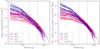 |
Fig. 1. Surface brightness (left panel) and self-similar scaled emission measure profiles (right panel) for HIFLUGCS objects with temperatures greater than 3 keV. Strong-cool-core, weak-cool-core, and non-cool-core clusters are labeled as SCC, WCC, and NCC, respectively. |
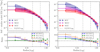 |
Fig. 2. Top panels: weighted mean (left panel) and median (right panel) self-similar scaled emission measure profiles for the individual core types of HIFLUGCS objects with temperatures greater than 3 keV. Bottom panels: Ratio of the self-similar scaled emission measure profiles between the different core type populations. Shown error bars were estimated with 10 000 bootstrapping iterations. The shaded regions represent the intrinsic scatter values of each bin. |
The weighted mean profiles reveal in a model-independent way the existence of subtle differences between the galaxy cluster populations. The amplitude of this effect between SCC and NCC clusters in the 0.2 − 0.5 r500 radial range is up to 30% and confirms the finding of Eckert et al. (2012). Compared to the heterogeneous sample of Eckert et al. (2012) HIFLUGCS is statistically complete, which confirms the result in a more robust way. If true, this finding implies that the outskirts are affected by the core-type and a detection algorithm tailored to the galaxy cluster outskirts will be more sensitive to the more abundant NCC objects, which needs to be taken into account in selection functions. In addition one could determine the statistical likelihood for the core-state of a particular galaxy cluster. However, the asymmetric bootstrap errors indicate an underlying non-Gaussian distribution or that the sample is affected by outliers. The median profiles, which are more robust against outliers, do not reveal the same trend of the emission measure ratios. As a test, we exclude the strong cool-core profile that deviates most with respect to the median within 0.2 − 0.5 r500 (Abell 3526). This cluster also shows the smallest statistical errors in this radial range. The weighted mean ratios resembles well the trend of the median when excluding this single cluster from the analysis. This reveals that the weighted mean is driven by an outlier with small statistical errors. Therefore, we conclude that there is no indication of a systematic core-type differences in the galaxy clusters 0.2 − 0.5 r500 radial range. Nevertheless, this comparison is useful because outliers like Abell 3526 will affect the selection function. The investigation of a possible redshift evolution of this analysis is left to a future study. Beyond 0.5 r500 the difference between SCC and NCC clusters become larger. Eckert et al. (2012) discussed gas redistribution between the core region and the outskirts as possible explanation. In this scenario, the injected energy due to a merging event flattens the density profile of interacting objects. Assuming that NCC clusters are more likely to have experienced a recent merging event, their self-similar scaled EM profiles would be different compared to CC objects. Another explanation could be the current accretion of large-scale blobs. Clusters with higher mass accretion rates show a larger fraction of non-thermal pressure in simulations (Nelson et al. 2014). Again assuming that NCC objects are merging clusters, the discrepancies can be explained by the different non-thermal energy content. However, this scenario seems unlikely since we expect to detect such structures in our wavelet images. An additional explanation can be that the dark matter halos of NCC and CC objects have different shapes and thus a different concentration at a given radius.
5. Large-scale center and ellipticity
The wavelet decomposition allows us to study galaxy cluster parameters on large scales. The one scale around 0.2 r500 is used to determine the center and ellipticities using the SExtractor program (Bertin & Arnouts 1996). This minimizes the impact of the different core states on these parameters. The chosen scale contains most of the cluster counts outside the core region and is therefore a good tracer for large-scale properties. Including scales up to around 0.5 r500 (an additional 1 − 3 scales) shows that the median and mean difference in ellipticity is just about 10%. The ellipticity, e, of an ellipse with major-axis, e1, and minor-axis, e2, is defined as
 (23)
(23)
and is shown as function of the cooling time in Fig. 3. The two parameters do not show a significant correlation (Spearman rank-order correlation coefficient of 0.17). The medians and sample standard deviations in the three bins are (0.24, 0.28, 0.25) and (0.08, 0.12, 0.14), respectively. There are no highly elliptical clusters with short cooling times. Therefore, selecting clusters above an ellipticity of approximately 0.3 creates a sample without SCC objects. The universality of this result needs to be confirmed with galaxy cluster samples of larger sizes.
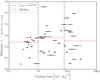 |
Fig. 3. Ellipticity as a function of central cooling time of HIFLUGCS objects with temperatures greater than 3 keV. Vertical dashed lines indicate cooling times corresponding to the cool-core classification. |
We perform a similar stacking analysis as in Sect. 4, where the sample is divided into 3 sub-classes according to ellipticity, rather than core-state. The weighted mean and median profiles are shown in Fig. 4. The median profiles do not show a difference between the sub-classes except in the core region and the very outskirts.
We quantify the covariance between ellipticity and core radius in kpc. For a core-modeled single β-model and fixed β-parameter, the Spearman rank-order correlation coefficient is 0.20, which is no strong indication for a correlation. Allowing the β-parameter to vary introduces a small positive correlation coefficient of 0.33. We see a similar behavior for best-fit core radii using a single β-model.
Clusters with large cooling times show a large range of 2D ellipticities. Assuming that they originate from the same population in 3D, the large scatter of ellipticity might be explained by projection effects, meaning that triaxial halos with random orientations will yield a wide range of observed 2D ellipticities. The verification of this effect using simulations is left to a future study. Considering ellipticity adds supplementary information since it is not significantly correlated with the core radius. The ellipticity in the galaxy cluster outskirts traces the amount of baryon dissipation (Lau et al. 2012). Thus, ellipticity is linked and may help to constrain cosmological parameters like the amplitude of the matter power spectrum, σ8. Halos form later for lower σ8 values and are therefore on average more elliptical (Allgood et al. 2006; Macciò et al. 2008). In addition, measuring ellipticity on several scales allows to indirectly study large-scale gas rotation in galaxy clusters (Bianconi et al. 2013). This allows us to test if the ICM is in hydrostatic equilibrium, an often made assumption in X-ray mass measurements. This makes the ellipticity an interesting survey measure for the future eROSITA X-ray all-sky survey, where we expect a range of ellipticities. The ratio of the weighted mean profiles between objects with low and high ellipticity shows a slight offset. Since this offset is not visible in the median profile, it cannot solely be explained by the larger non-Gaussianity per bin of elliptical surface brightness distributions extracted in circular annuli.
Hashimoto et al. (2007) studied the relationships between the X-ray morphology and several other cluster properties using a heterogeneous sample of 101 clusters taken from the Chandra archive, out of which 18 objects are represented in HIFLUGCS. The ellipticity measurements are in agreement with our study within a factor of approximately two, except for A0399. For this cluster, the ellipticity calculated by Hashimoto et al. (2007) is a factor of 5.6 larger (0.284 compared to 0.051). We note that the semi-major and semi-minor axis are calculated in the same way, that is by the 2nd-order moments but we subtracted the central excess emission of the cluster before. Including the central excess emission brings our results in better agreement with Hashimoto et al. (2007), especially in the case of A0399. For a single β-model description of the surface brightness profile, they find a slightly larger Spearman rank-order correlation coefficient of 0.37, compared to 0.26, between ellipticity and core radius in kpc.
6. Analysis of the residuals
In this section we quantify how well the different model parameterizations represent the underlying HIFLUGCS surface brightness profiles. All profiles are fitted over the full extracted radial range (see Fig. D.1) using an MCMC posterior sampling technique, taking uncertainties in the measured surface brightness into account. In case of the core-modeled single β-model all contaminating sources, including the excess emission in the cluster core, are modeled according to Eq. (5). For the single β-model fitting procedure we perform a classical approach of masking contaminating sources that are detected on the wavelet images. This includes point-like sources or extended emission like substructure but not emission from the cluster core. Thus the likelihood functions for the two cases are different because for a single β-model, Bwv, i in Eq. (5) is equal to zero for all i. The choice of priors is discussed in Appendix B. The background is modeled with an additive constant. We note that not subtracting the background before fitting introduces a positive degeneracy between the best-fit slope of the β-model and the background level. In this framework, residuals are defined as (data-model)/model, meaning that positive (negative) residuals indicate that the model under- (over-) predicts the observed surface brightnesses. We focus particularly on the 0.2 − 0.5 r500 radial range because most of the galaxy cluster counts outside the non-scalable core regions are expected there.
6.1. Discussion: Single β-models
A single β-model is a widely used description to fit surface brightness profiles, especially in the low statistics regime. Therefore, it is also commonly used to detect extended sources in X-ray surveys. In Fig. 5 (top left panel), we show the fractional median of the residuals from a single β-model in the 0.2 − 0.5 r500 radial range as function of core radius. There is a clear trend of positive residuals toward smaller core radii. This means that the flux in the outskirts is systematically under-predicted, especially for SCC objects (see Sect. 6.3). In addition, the core radii of objects that exhibit cool-cores are systematically biased low since a single β-model lacks degrees of freedom to model the central excess emission. Due to higher photon statistics in the core region, a single β-model fit tends to be driven by the inner radial bins. As an additional test we reduce the weight of the core region in the fitting procedure by assuming that the variance in the Gaussian likelihood function is underestimated by a given fractional amount f = 0.1. The qualitative behavior of the residuals remains the same. In cases where the cluster outskirts are poorly fitted, the background level is not determined properly as well because its level compensates for the poor fit in the outskirts. This influences the β value determination as already discussed. The median of the β parameters is 0.59 and thus smaller than the often assumed generic value of 2/3. The best-fit values of the surface brightness parameters are in good agreement with Reiprich & Böhringer (2002).
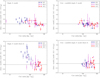 |
Fig. 5. Median of the fractional residuals from a single β-model (left panels) and a core-modeled single β-model (right panels) in 0.2 − 0.5 r500 radial bins for individual HIFLUGCS objects above a temperature of 3 keV as function of core radius. Bottom panels: β parameter is fixed to 2/3 in the surface brightness parameter optimization. |
The single β-model residuals for individual clusters have a wavy form. We investigate different functional forms to describe the common deviations from a single β-model, but no significant common form of the residuals could be found. The scatter around zero and bias in the 0.2 − 0.5 r500 radial bin are 0.092 and 0.032 ± 0.003, respectively. The non-zero bias reflects the same finding as discussed above.
The residuals in the 0.2 − 0.5 r500 radial range from a single β-model with fixed β parameter (β = 2/3) is shown in the bottom left panel of Fig. 5. The amplitude of the residuals for SCC objects increases up to over 40%. Fixing the β parameter increases the scatter and bias to 0.161 and 0.066 ± 0.003, respectively.
6.2. Discussion: Core-modeled single β-models
The negative effects of a single β-model as described in Sect. 6.1 are reduced when modeling the excess core emission by adding the counts on the small scales of the wavelet decomposition to the model counts in the Poisson likelihood function (see Sect. 3.1.2). The residuals in the 0.2 − 0.5 r500 radial range are shown in Fig. 5 (top right panel). The measured residuals scatter around zero and there is no bias between individual core types visible. The scatter around zero in the 0.2 − 0.5 r500 radial bin is slightly reduced compared to the single β-model (0.074). Most importantly, the bias gets more consistent with zero (−0.004 ± 0.003). In case of a fixed β parameter (bottom right panel of Fig. 5), the bias of a core-modeled single β-model is consistent with zero (−0.001 ± 0.003) and the scatter is slightly increased (0.087). The median of the β parameters is larger compared to the single β-model case and with 0.696 close to the generic value of 2/3.
To verify our core-modeling method and to confirm its results we excise the core region (< 0.2 r500) in the single β-model fitting procedure. This is an independent way to avoid the single β-model fit to be driven by the non-scalable core emission and to reduce residuals between model and data in the cluster outskirts. In more than 90% of the cases, we find that this approach delivers comparable best-fit parameters for β and core-radii as when modeling the core emission. Due to excluding data, the constraining power is reduced and the degeneracy of the shape parameters with the β-model normalization is larger. In several cases, this results in a larger mismatch of the β-model fluxes compared to the real flux of the objects.
6.3. Flux comparison
This section compares the overall model flux, as well as the model flux in the cluster outskirts for the single β-model and core-modeled single β-model to the measured flux in the corresponding radial range. For each model, we calculate the cluster count rate by integrating a single β-model with the corresponding best-fit parameters in a given radial range, that is 0 − rx (the outer significance radius) for the overall model flux and 0.2 − 0.5 r500 for the flux in the outskirts. We are interested in flux ratios, in which the count rate to flux conversion factors of individual clusters cancel each other out. We calculate the total flux of the single β-model including the central excess emission and subtract the wavelet-detected central excess emission in the core-modeled case. The median of the measured fluxes in the outskirts and the overall fluxes of the NCC and WCC objects agree very well with each other. The measured overall single β-model fluxes of the SCC objects are on average approximately 23% larger compared to the measured overall core-modeled fluxes and the flux ratio has an intrinsic scatter of approximately 14% around the median. The median accuracy between model and measured total flux is within approximately 4% (2%) for the (core-modeled) single β-model, regardless of the core-type or if the β value is free to vary or fixed to 2/3. The flux in the outskirts of the core-modeled single β-model has the same median accuracy of 2%. For the single β-model, the accuracy stays at the 4% level for WCC and NCC objects. For SCC objects, for the single beta-model case, the flux in the outskirts is biased low by 6% and increases to 10% when β is fixed to 2/3; meaning that the bias is 3 − 5 times larger than for the core-modeled case. In all cases, the intrinsic scatter values of the ratios are below 6%. The Spearman rank-order correlation coefficients do not reveal a significant correlation between the flux underestimation and the cluster temperature.
7. Scaling relations
This section describes how the shape parameters scale with temperature and how they correlate with luminosity. In Fig. 6, we show the core radius as a function of temperature, where the β parameter is fixed to 2/3 to avoid degeneracies between the surface brightness parameters. We note that the overall picture does not change when fixing β to the median of the full population or the medians of the individual core-type populations. To account for a possible temperature dependence, the core radii are divided by the square-root of the corresponding cluster temperatures (see below for more details). The figure emphasizes the systematic differences between the individual core types in the modeling with a single β-model. The discrepancies get less prominent when modeling the core region using the wavelet decomposition. In addition, the intrinsic scatter is reduced by 8%, 11%, and 35% for NCC, WCC, and SCC objects, respectively. In both modeling cases, the Spearman rank-order correlation coefficients indicate a stronger negative (−0.7), a mild positive (0.3) and no significant (0) correlation for the NCC, WCC, and SCC populations, respectively.
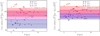 |
Fig. 6. Core radius as a function of temperature for a single β-model (left panel) and core-modeled (right panel) single β-model. The dashed lines and shaded regions represent the medians and their intrinsic scatter of the individual core populations. |
We determine scaling relations as outlined in Sect. 3.4. The best-fit relations between shape parameters and temperature (Fig. 7), as well as luminosity and temperature are determined simultaneously. This allows studying the covariances between shape and luminosity from the joint fit. The best-fit values are shown in Tables 1 and 2. In Fig. 8, we show the correlation between the shape parameters and luminosity. The Spearman rank-order correlation coefficients between luminosity and β, as well as luminosity and core radius are 0.37 and 0.12 (0.32 and 0.22) for the (core-modeled) single β-model, respectively. When the β value is fixed to 2/3, the luminosity-core radius correlation coefficients become mildly negative with −0.23 (−0.22).
Parameters from single β-model and core-modelled single β-model fits to the y-temperature scaling relations.
Correlation coefficients between different galaxy cluster parameters from single β-model and core-modelled single β-model fits.
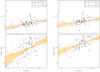 |
Fig. 7. Scaling relations between single β-model (left panels) and core-modeled single β-model (right panels) parameters and temperature. The HIFLUGCS clusters with temperatures greater than 3 keV (black points) are used for optimization. Red points mark HIFLUGCS objects below this temperature threshold for visualization. The orange lines and shaded regions show the best-fit relations and their uncertainties, respectively. The blue dashed lines correspond to the intrinsic log-normal scatter. |
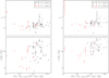 |
Fig. 8. Single β-model (left panels) and core-modeled single β-model (right panels) parameters as a function of luminosity. The HIFLUGCS clusters with temperatures greater than and below 3 keV are marked as black and red points, respectively. |
The best-fit parameters of the single β-model and core-modeled single β-model scaling relations agree approximately on the 1σ level, except that in the latter case the intrinsic scatter value of the core radius is reduced by almost a factor of two. In both modeling approaches the shape parameters show a positive correlation with temperature. The shape parameters of galaxy clusters are often fixed to generic values (e.g., β = 2/3) or scaling relations (e.g., rc ∝ r500, Pacaud et al. 2018). The assumption that the core-radius is proportional to r500, together with Eq. (10) results in a self-similar scaling of rc ∝ T1/2. We find a core-radius-temperature relation with a marginally steeper slope of 1.04 ± 0.37 (0.75 ± 0.20) for the (core-modeled) single β-model compared to this expectation. Fixing the value of β to 2/3 results in 0.77 ± 0.14 (0.50 ± 0.16), consistent with the self-similar value when modeling the excess core emission. We study the correlation coefficients (Table 2) between the different galaxy cluster parameters by simultaneously fitting for the scaling relations and the intrinsic scatter tensor. We expect some degeneracy between the single β-model parameters in the fitting, amongst others that a larger core-radius is compensated by a steeper slope. This is reflected in the strong positive correlation between core-radius and β. We do not find a significant correlation between β and luminosity. There is a strong negative correlation between core radius and luminosity, meaning that at a given temperature, more luminous objects tend to be more compact. For all modeling cases, the best-fit correlation coefficients are consistent on a 1σ level. This implies, that the measured correlation between core radius and luminosity is not significantly affected by modeling the central excess emission. Neither this covariance nor the shape-temperature relations are taken into account in existing simulations for eROSITA but may play a crucial role in understanding selection effects related to the detection of clusters in X-ray surveys, which is a key ingredient for using X-ray galaxy clusters as a precision cosmological probe. The findings presented here can be used to perform more realistic simulations and a comparison between different sets of simulations allows to study the impact of these covariances on obtained cosmological parameters.
8. Summary
X-ray morphologies of galaxy clusters play a crucial role in the determination of the survey selection function. We compare self-similar scaled emission measure profiles of a well defined galaxy cluster sample (HIFLUGCS) above a representative temperature threshold of 3 keV. One outlier (Abell 3526) with small statistical errors drives the weighted mean profiles of sub-populations according to different core properties toward a different behavior of strong cool-core and non-cool-core objects in the 0.2 − 0.5 r500 radial range. Excluding this object from the analysis or calculating the median profiles reveals no systematic difference in the aforementioned radial range. We conclude that there is no indication for a correlation between the behavior in the 0.2 − 0.5 r500 radial range and the core state, although the overall shapes of the SCC and NCC populations are different. The median SCC profile shows a larger normalization toward the center and is steeper compared to the median NCC profile. This leads to a turnover of the profile ratio at approximately 0.3 r500. The difference in the center can be explained by the core state but the difference in the outskirts is still under debate. As discussed in Sect. 4 possible explanations are gas redistribution between the core region and the outskirts, the current accretion of large-scale blobs, or different shapes of the dark matter halos leading to different concentrations at a given radius. Characterizing galaxy cluster surface brightness profiles with single β-models is still state-of-the-art in the determination of selection functions. We investigate the residuals of a single β-model fit to the overall cluster profile, revealing that this description tends to underestimate the flux in the galaxy cluster outskirts for less extended clusters. Fixing the β parameter to 2/3 increases this effect dramatically, that is up to over 40%. In both cases, the core-radius measurement for SCC objects are biased low. In addition, the intrinsic scatter values with respect to the medians of the self-similar scaled extent parameters show a more than 1σ tension between strong and non-cool-core objects. These three effects can be minimized by adapting a wavelet decomposition based surface brightness modeling that is sensitive to the galaxy cluster outskirts and models the excess emission in the core region. Then, the fit is not driven by the local processes in the core. Compared to a single β-model approach the residuals in the 0.2 − 0.5 r500 radial range are much smaller and the core radii depend much more mildly on the core state. Our method to model the excess core emission has very interesting applications for future galaxy cluster surveys, for example with eROSITA. The performance study for high redshift objects with small angular extent and establishing the most robust method for clusters where r500 is unknown is left to a future work. Using wavelet decomposition allows to determine large-scale ellipticities of the clusters. The ellipticity is an interesting new survey measure for eROSITA since it’s determination does not require many photon counts and it adds additional information to the β-model shape parameters and core-excised luminosities. A detailed study of measuring galaxy cluster ellipticities with eROSITA and it’s implications is left to a future work.
We study how shape parameters and luminosity scale with temperature. There is no significant difference of the best-fit values between a single β-model and core-modeled single β-model, except that the intrinsic scatter of the core radius is almost twice as large for the single β-model case. The slope of the core radius-temperature relation is steeper than the self-similar prediction of 1/2 but gets in agreement when fixing the β parameter to 2/3 in the surface brightness profile modeling. More interestingly, the shape parameters are covarient with luminosity, meaning that at a given temperature, more compact objects are more luminous. These covariances are usually neglected in simulations to determine the survey selection function (Pacaud et al. 2007; Clerc et al. 2018). In addition, these previous studies assumed a fixed β value, while we find that β is a function of temperature. Taking shape-temperature scaling relations and shape-luminosity covariances into account will lead to a more realistic set of simulated galaxy clusters and will provide a better understanding of the survey completeness.
X-ray gas temperatures are often expressed in kiloelectronvolt (keV). Using the Boltzmann constant kB, 1 keV/kB ≈ 1.16 × 10⁷ K.
We note that the assumption of single β-models is that the hot gas and the galaxies are in hydrostatic equilibrium and isothermal.
Please contact A. Vikhlinin for the latest version of ZHTOOLS (This email address is being protected from spambots. You need JavaScript enabled to view it. ).
Acknowledgments
This research was made possible by the International Max Planck Research School on Astrophysics at the Ludwig-Maximilians University Munich, as well as their funding received from the Max-Planck Society.
References
- Allgood, B., Flores, R. A., Primack, J. R., et al. 2006, MNRAS, 367, 1781 [NASA ADS] [CrossRef] [Google Scholar]
- Anders, E., & Grevesse, N. 1989, Geochim. Cosmochim. Acta, 53, 197 [Google Scholar]
- Arnaud, M., Aghanim, N., & Neumann, D. M. 2002, A&A, 389, 1 [NASA ADS] [CrossRef] [EDP Sciences] [Google Scholar]
- Bartelmann, M., & Steinmetz, M. 1996, MNRAS, 283, 431 [NASA ADS] [Google Scholar]
- Bertin, E., & Arnouts, S. 1996, A&AS, 117, 393 [NASA ADS] [CrossRef] [EDP Sciences] [Google Scholar]
- Bianconi, M., Ettori, S., & Nipoti, C. 2013, MNRAS, 434, 1565 [NASA ADS] [CrossRef] [Google Scholar]
- Boese, F. G. 2000, A&AS, 141, 507 [NASA ADS] [CrossRef] [EDP Sciences] [Google Scholar]
- Böhringer, H., Voges, W., Huchra, J. P., et al. 2000, ApJS, 129, 435 [NASA ADS] [CrossRef] [Google Scholar]
- Bryan, G. L., & Norman, M. L. 1998, ApJ, 495, 80 [NASA ADS] [CrossRef] [Google Scholar]
- Cash, W. 1979, ApJ, 228, 939 [NASA ADS] [CrossRef] [Google Scholar]
- Cavaliere, A., & Fusco-Femiano, R. 1976, A&A, 49, 137 [NASA ADS] [Google Scholar]
- Chen, Y., Reiprich, T. H., Böhringer, H., Ikebe, Y., & Zhang, Y.-Y. 2007, A&A, 466, 805 [NASA ADS] [CrossRef] [EDP Sciences] [Google Scholar]
- Clerc, N., Ramos-Ceja, M. E., Ridl, J., et al. 2018, A&A, 617, A92 [NASA ADS] [CrossRef] [EDP Sciences] [Google Scholar]
- Eckert, D., Molendi, S., & Paltani, S. 2011, A&A, 526, A79 [NASA ADS] [CrossRef] [EDP Sciences] [Google Scholar]
- Eckert, D., Vazza, F., Ettori, S., et al. 2012, A&A, 541, A57 [NASA ADS] [CrossRef] [EDP Sciences] [Google Scholar]
- Foreman-Mackey, D., Hogg, D. W., Lang, D., & Goodman, J. 2013, PASP, 125, 306 [CrossRef] [Google Scholar]
- Ghirardini, V., Eckert, D., Ettori, S., et al. 2019, A&A, 621, A41 [NASA ADS] [CrossRef] [EDP Sciences] [Google Scholar]
- Giodini, S., Lovisari, L., Pointecouteau, E., et al. 2013, Space Sci. Rev., 177, 247 [NASA ADS] [CrossRef] [Google Scholar]
- Greiner, J., Burgess, J. M., Savchenko, V., & Yu, H.-F. 2016, ApL, 827, 38 [Google Scholar]
- Hashimoto, Y., Böhringer, H., Henry, J. P., Hasinger, G., & Szokoly, G. 2007, A&A, 467, 485 [NASA ADS] [CrossRef] [EDP Sciences] [Google Scholar]
- Hudson, D. S., Mittal, R., Reiprich, T. H., et al. 2010, A&A, 513, A37 [NASA ADS] [CrossRef] [EDP Sciences] [Google Scholar]
- Kaiser, N. 1986, MNRAS, 222, 323 [NASA ADS] [CrossRef] [Google Scholar]
- Kelly, B. C. 2007, ApJ, 665, 1489 [NASA ADS] [CrossRef] [Google Scholar]
- King, I. 1962, AJ, 67, 471 [NASA ADS] [CrossRef] [Google Scholar]
- Kravtsov, A. V., Vikhlinin, A., & Nagai, D. 2006, ApJ, 650, 128 [NASA ADS] [CrossRef] [Google Scholar]
- Lau, E. T., Nagai, D., Kravtsov, A. V., Vikhlinin, A., & Zentner, A. R. 2012, ApJ, 755, 116 [NASA ADS] [CrossRef] [Google Scholar]
- Lin, H. W., McDonald, M., Benson, B., & Miller, E. 2015, ApJ, 802, 34 [NASA ADS] [CrossRef] [Google Scholar]
- Macciò, A. V., Dutton, A. A., & van den Bosch, F. C. 2008, MNRAS, 391, 1940 [NASA ADS] [CrossRef] [Google Scholar]
- Mantz, A., Allen, S. W., Ebeling, H., Rapetti, D., & Drlica-Wagner, A. 2010, MNRAS, 406, 1773 [NASA ADS] [Google Scholar]
- Mantz, A. B., Allen, S. W., Morris, R. G., et al. 2016, MNRAS, 463, 3582 [NASA ADS] [CrossRef] [Google Scholar]
- Maughan, B. J. 2007, ApJ, 668, 772 [NASA ADS] [CrossRef] [Google Scholar]
- Maughan, B. J., Giles, P. A., Randall, S. W., Jones, C., & Forman, W. R. 2012, MNRAS, 421, 1583 [NASA ADS] [CrossRef] [Google Scholar]
- Merloni, A., Predehl, P., Becker, W., et al. 2012, ArXiv e-prints [arXiv:1209.3114] [Google Scholar]
- Mittal, R., Hicks, A., Reiprich, T. H., & Jaritz, V. 2011, A&A, 532, A133 [NASA ADS] [CrossRef] [EDP Sciences] [Google Scholar]
- Navarro, J. F., Frenk, C. S., & White, S. D. M. 1995, MNRAS, 275, 720 [NASA ADS] [CrossRef] [Google Scholar]
- Navarro, J. F., Frenk, C. S., & White, S. D. M. 1996, A&A, 462, 563 [Google Scholar]
- Navarro, J. F., Frenk, C. S., & White, S. D. M. 1997, A&A, 490, 493 [Google Scholar]
- Nelson, K., Lau, E. T., & Nagai, D. 2014, ApJ, 792, 25 [NASA ADS] [CrossRef] [Google Scholar]
- Pacaud, F., Pierre, M., Adami, C., et al. 2007, MNRAS, 382, 1289 [NASA ADS] [CrossRef] [Google Scholar]
- Pacaud, F., Pierre, M., Melin, J.-B., et al. 2018, A&A, 620, A10 [NASA ADS] [CrossRef] [EDP Sciences] [Google Scholar]
- Planck Collaboration XI. 2016, A&A, 594, A27 [NASA ADS] [CrossRef] [EDP Sciences] [Google Scholar]
- Pratt, G. W., Croston, J. H., Arnaud, M., & Böhringer, H. 2009, A&A, 498, 361 [NASA ADS] [CrossRef] [EDP Sciences] [Google Scholar]
- Predehl, P., Bornemann, W., Bräuninger, H., et al. 2018, SPIE Conf. Ser., 10699, 106995H [Google Scholar]
- Reiprich, T. H., & Böhringer, H. 2002, ApJ, 567, 716 [NASA ADS] [CrossRef] [Google Scholar]
- Rossetti, M., Gastaldello, F., Eckert, D., et al. 2017, MNRAS, 468, 1917 [NASA ADS] [CrossRef] [Google Scholar]
- Sanderson, A. J. R., Ponman, T. J., & O’Sullivan, E. 2006, MNRAS, 372, 1496 [NASA ADS] [CrossRef] [Google Scholar]
- Santos, J. S., Rosati, P., Tozzi, P., et al. 2008, A&A, 483, 35 [NASA ADS] [CrossRef] [EDP Sciences] [Google Scholar]
- Schellenberger, G., & Reiprich, T. H. 2017, MNRAS, 469, 3738 [NASA ADS] [CrossRef] [Google Scholar]
- Snowden, S. L., McCammon, D., Burrows, D. N., & Mendenhall, J. A. 1994, ApJ, 424, 714 [NASA ADS] [CrossRef] [Google Scholar]
- VanderPlas, J. 2016, Python Data Science Handbook: Essential Tools for Working with Data, 1st edn. (O’Reilly Media, Inc.) [Google Scholar]
- Vikhlinin, A., McNamara, B. R., Forman, W., et al. 1998, Astrophysical Journal, 502, 558 [Google Scholar]
- Vikhlinin, A., Forman, W., & Jones, C. 1999, ApJ, 525, 47 [NASA ADS] [CrossRef] [Google Scholar]
- Vikhlinin, A., Burenin, R., Forman, W. R., et al. 2007, in Heating versus Cooling in Galaxies and Clusters of Galaxies, eds. H. Böhringer, G. W. Pratt, A. Finoguenov, P. Schuecker, 48 [CrossRef] [Google Scholar]
- Voges, W., Aschenbach, B., Boller, T., et al. 1999, A&A, 349, 389 [NASA ADS] [Google Scholar]
- Willingale, R., Starling, R. L. C., Beardmore, A. P., Tanvir, N. R., & O’Brien, P. T. 2013, MNRAS, 431, 394 [NASA ADS] [CrossRef] [Google Scholar]
- Zhang, Y.-Y., Finoguenov, A., Böhringer, H., et al. 2007, A&A, 467, 437 [NASA ADS] [CrossRef] [EDP Sciences] [Google Scholar]
Appendix A: Mass comparison
In this section we compare our previous emission measure ratio results of Sect. 4 to profiles that are re-scaled by a characteristic radii according to hydrostatic mass estimates by Schellenberger & Reiprich (2017). We adapt their preferred “NFW Freeze” model, where a NFW profile (Navarro et al. 1996, 1997) is fit to the outermost measured mass profiles of Chandra observations and a concentration-mass relation is used to reduce the degrees of freedom. We are interested in the difference between individual core-types and not in the bias between the Planck and hydrostatic masses. Therefore, we assume that the bias is constant for all clusters. To probe the masses at the same radii, we recalculate the hydrostatic masses at the Planck r500 values according to Formula (31) of Schellenberger & Reiprich (2017)
 (A.1)
(A.1)
where c500 denotes the NFW concentration parameter and Y(u)=ln(1 + u)−u/(1 + u). These recalculated masses are on average lower than the corresponding masses in the Planck catalog. The median of the NCC cluster masses is approximately 13% larger than that of the SCC objects (see Fig. A.1), increasing the SCC to NCC weighted mean ratio effect in the 0.2 − 0.5 r500 range to 40%. This increase due to the dynamical states is also seen in simulations, for example in different fractions of non-thermal pressure for different mass accretion rates (Nelson et al. 2014). The differences can thus be explained by assuming that NCC clusters are merging objects and that they contain more non-thermal energy. An alternative explanation is that the differences come from the assumed concentration-mass relation. We expect different core-types to have different shapes of the dark matter halo and therefore different concentrations at a given radius. However, fitting for the concentration in Schellenberger & Reiprich (2017) results in some cases to unrealistic high or low masses, potentially because of limited radial coverage due to the relatively small Chandra field-of-view.
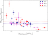 |
Fig. A.1. Comparison between Planck and hydrostatic mass estimates of HIFLUGCS objects with temperatures greater than 3 keV. |
Appendix B: Priors
We list the priors used for this analysis in Table B.1. They are chosen to be weakly- or non-informative and varying them does not influence the results of this study significantly.
List of parameters and their priors.
Appendix C: HIFLUGCS parameters
Galaxy cluster parameters.
Appendix D: HIFLUGCS images and surface brightness profiles
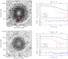 |
Fig. D.1. Left panels: ROSAT count rate images for individual galaxy clusters. The large-scale centers are shown as green plus signs. Red contours correspond to wavelet scales used for background modeling. The large scales (the ones above 0.2 r500) are shown as blue contours. These large scales are used to calculate the center and ellipticities. The extracted SExtractor ellipses are displayed in dashed green. Each box size corresponds to the outer significance radius of the shown cluster. Right panels: top panels show the measured (black points) surface brightness profiles of individual galaxy clusters. The background models used for the single β-model fits (solid blue lines) are shown as red points. Bottom panels: residuals of the core-modelled single β-model fits. |
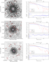 |
Fig. D.1. continued. |
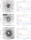 |
Fig. D.1. continued. |
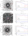 |
Fig. D.1. continued. |
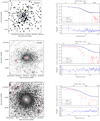 |
Fig. D.1. continued. |
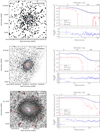 |
Fig. D.1. continued. |
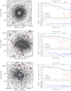 |
Fig. D.1. continued. |
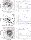 |
Fig. D.1. continued. |
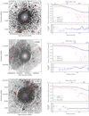 |
Fig. D.1. continued. |
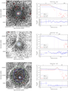 |
Fig. D.1. continued. |
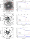 |
Fig. D.1. continued. |
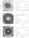 |
Fig. D.1. continued. |
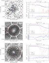 |
Fig. D.1. continued. |
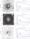 |
Fig. D.1. continued. |
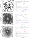 |
Fig. D.1. continued. |
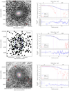 |
Fig. D.1. continued. |
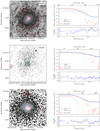 |
Fig. D.1. continued. |
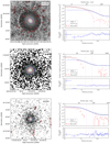 |
Fig. D.1. continued. |
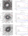 |
Fig. D.1. continued. |
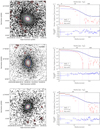 |
Fig. D.1. continued. |
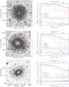 |
Fig. D.1. continued. |
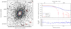 |
Fig. D.1. continued. |
All Tables
Parameters from single β-model and core-modelled single β-model fits to the y-temperature scaling relations.
Correlation coefficients between different galaxy cluster parameters from single β-model and core-modelled single β-model fits.
All Figures
|
Fig. 1. Surface brightness (left panel) and self-similar scaled emission measure profiles (right panel) for HIFLUGCS objects with temperatures greater than 3 keV. Strong-cool-core, weak-cool-core, and non-cool-core clusters are labeled as SCC, WCC, and NCC, respectively. |
| In the text | |
|
Fig. 2. Top panels: weighted mean (left panel) and median (right panel) self-similar scaled emission measure profiles for the individual core types of HIFLUGCS objects with temperatures greater than 3 keV. Bottom panels: Ratio of the self-similar scaled emission measure profiles between the different core type populations. Shown error bars were estimated with 10 000 bootstrapping iterations. The shaded regions represent the intrinsic scatter values of each bin. |
| In the text | |
|
Fig. 3. Ellipticity as a function of central cooling time of HIFLUGCS objects with temperatures greater than 3 keV. Vertical dashed lines indicate cooling times corresponding to the cool-core classification. |
| In the text | |
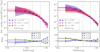 |
Fig. 4. Same as Fig. 2, except that the classification is done according to ellipticity. |
| In the text | |
|
Fig. 5. Median of the fractional residuals from a single β-model (left panels) and a core-modeled single β-model (right panels) in 0.2 − 0.5 r500 radial bins for individual HIFLUGCS objects above a temperature of 3 keV as function of core radius. Bottom panels: β parameter is fixed to 2/3 in the surface brightness parameter optimization. |
| In the text | |
|
Fig. 6. Core radius as a function of temperature for a single β-model (left panel) and core-modeled (right panel) single β-model. The dashed lines and shaded regions represent the medians and their intrinsic scatter of the individual core populations. |
| In the text | |
|
Fig. 7. Scaling relations between single β-model (left panels) and core-modeled single β-model (right panels) parameters and temperature. The HIFLUGCS clusters with temperatures greater than 3 keV (black points) are used for optimization. Red points mark HIFLUGCS objects below this temperature threshold for visualization. The orange lines and shaded regions show the best-fit relations and their uncertainties, respectively. The blue dashed lines correspond to the intrinsic log-normal scatter. |
| In the text | |
|
Fig. 8. Single β-model (left panels) and core-modeled single β-model (right panels) parameters as a function of luminosity. The HIFLUGCS clusters with temperatures greater than and below 3 keV are marked as black and red points, respectively. |
| In the text | |
|
Fig. A.1. Comparison between Planck and hydrostatic mass estimates of HIFLUGCS objects with temperatures greater than 3 keV. |
| In the text | |
|
Fig. D.1. Left panels: ROSAT count rate images for individual galaxy clusters. The large-scale centers are shown as green plus signs. Red contours correspond to wavelet scales used for background modeling. The large scales (the ones above 0.2 r500) are shown as blue contours. These large scales are used to calculate the center and ellipticities. The extracted SExtractor ellipses are displayed in dashed green. Each box size corresponds to the outer significance radius of the shown cluster. Right panels: top panels show the measured (black points) surface brightness profiles of individual galaxy clusters. The background models used for the single β-model fits (solid blue lines) are shown as red points. Bottom panels: residuals of the core-modelled single β-model fits. |
| In the text | |
|
Fig. D.1. continued. |
| In the text | |
|
Fig. D.1. continued. |
| In the text | |
|
Fig. D.1. continued. |
| In the text | |
|
Fig. D.1. continued. |
| In the text | |
|
Fig. D.1. continued. |
| In the text | |
|
Fig. D.1. continued. |
| In the text | |
|
Fig. D.1. continued. |
| In the text | |
|
Fig. D.1. continued. |
| In the text | |
|
Fig. D.1. continued. |
| In the text | |
|
Fig. D.1. continued. |
| In the text | |
|
Fig. D.1. continued. |
| In the text | |
|
Fig. D.1. continued. |
| In the text | |
|
Fig. D.1. continued. |
| In the text | |
|
Fig. D.1. continued. |
| In the text | |
|
Fig. D.1. continued. |
| In the text | |
|
Fig. D.1. continued. |
| In the text | |
|
Fig. D.1. continued. |
| In the text | |
|
Fig. D.1. continued. |
| In the text | |
|
Fig. D.1. continued. |
| In the text | |
|
Fig. D.1. continued. |
| In the text | |
|
Fig. D.1. continued. |
| In the text | |
Current usage metrics show cumulative count of Article Views (full-text article views including HTML views, PDF and ePub downloads, according to the available data) and Abstracts Views on Vision4Press platform.
Data correspond to usage on the plateform after 2015. The current usage metrics is available 48-96 hours after online publication and is updated daily on week days.
Initial download of the metrics may take a while.