| Issue |
A&A
Volume 628, August 2019
|
|
|---|---|---|
| Article Number | A73 | |
| Number of page(s) | 17 | |
| Section | Interstellar and circumstellar matter | |
| DOI | https://doi.org/10.1051/0004-6361/201834923 | |
| Published online | 08 August 2019 | |
Chemical and radiative transfer modeling of propylene oxide
Indian Centre for Space Physics,
43 Chalantika, Garia Station Road,
Kolkata
700084,
India
e-mail: This email address is being protected from spambots. You need JavaScript enabled to view it.
Received:
19
December
2018
Accepted:
10
June
2019
Abstract
Context. The recent identification of the first complex chiral molecule, propylene oxide (PrO), in space opens up a new window to further study the origin of homochirality on the Earth. There are some recent studies to explain the formation of PrO however additional studies on the formation of this species are needed for better understanding.
Aims. We seek to prepare a complete reaction network to study the formation of propylene oxide in the astrophysically relevant conditions. Based on our results, a detailed radiative transfer modeling has been carried out to propose some more transitions that would potentially be targeted in the millimeter wave domain.
Methods. A gas-grain chemical network was used to explain the observed abundance of PrO in a cold shell surrounding the high-mass star-forming region of Sgr B2. Quantum chemical calculations were employed to study various reaction parameters and to compute multiple vibrational frequencies of PrO.
Results. To model the formation of PrO in the observed region, we considered a dark cloud model. Additionally, we used a model to check the feasibility of forming PrO in the hot core region. Some potential transitions in the millimeter wave domain are predicted that could be useful for the future astronomical detection. We used radiative transfer modeling to extract the physical condition that might be useful to know the properties of the source in detail. Moreover, we provided vibrational transitions of PrO, which could be very useful for the future detection of PrO by the upcoming James Webb Space Telescope.
Key words: astrochemistry / methods: numerical / ISM: abundances / ISM: molecules / line: identification
© ESO 2019
1 Introduction
The discovery of a large number of complex interstellar species have significantly improved our understanding of the chemical processes involved in the interstellar medium (ISM). It is speculated that the building blocks of life (biomolecules) were formed in the ISM and were delivered by the comets to the Earth in the later stages (Chyba et al. 1990; Raymond et al. 2004; Hartogh et al. 2011). These life-making primordial organic compounds may also have been formed in the pre-solar nebula rather than on the early Earth (Bailey et al. 1998; Chakrabarti & Chakrabarti 2000a,b; Hunt-Cunningham & Jones 2004; Holtom et al. 2005; Buse et al. 2006; Herbst & van Dishoeck 2009). The prospect of extraterrestrial origin of biomolecules is a fascinating topic since many biomolecules are chiral. Synthesis and detection of prebiotic molecules in the ISM have been studied and discussed by various authors (Cunningham et al. 2007; Das et al. 2008a; Gupta et al. 2011; Majumdar et al. 2012; Garrod & Herbst 2006; Nuevo et al. 2014; Chakrabarti et al. 2015). In between the living organisms on the Earth, amino acids and sugars are chiral. Interestingly, most of the amino acids of terrestrial proteins and sugars found on the Earth are homochiral; amino acids are left-handed whereas sugars are right-handed. When and how this homochirality developed on the Earth is a matter of debate (Cohen et al. 1995). Various biomolecules were identified in the Murchison meteorite. Interestingly, an excess amount of L-amino acids were identified (Engel & Nagy 1982; Engel & Macko 1997), which also suggest an extraterrestrial source for molecular asymmetry in the solar system. Thus, observation of more chiral species along with their enantiomeric excess in space could be very useful for the better understanding of the origin of homochirality. But unfortunately, with the present observational facility, it is very difficult to define the enantiomeric excess of an interstellar species.
Cunningham et al. (2007) attempted to observe PrO in the Orion KL and Sgr B2(LMH) using the Mopra Telescope. Based on their observational results, they predicted an upper limit on the column density (~6.7 × 1014 cm−2) of PrO in the Sgr B2 (LMH) and predicted an excitation temperature of 200 K with a compact source size of 5″. Recently, McGuire et al. (2016) attempted to search for the existence of a complex chiral species in space. They targeted star-forming regions such as Sgr B2 with Parkes Observatory and Green Bank Telescope (GBT) and successfully identified the first complex chiral molecule (PrO) in space. They were unable to determine the enantiomeric excess of PrO because of the lack of high precision and full polarization state measurement. McGuire et al. (2016) identified three transitions of PrO in absorption that correspond to the excitation temperature of ~5 K and column density ~1 × 1013 cm−2.
PrO has a significant proton affinity (Hunter & Lias 1998) and should be converted into protonated form through some ion-neutral (IN) reactions. Panels a, b, and c of Fig. 1 depict the structure of PrO and its two protonated forms, respectively. Swalen & Hershbach (1957) and Hershbach & Swalen (1958) discussed the internal barrier of PrO and its various rotational transitions in the ground and torsionally excited states. Later, Creswell & Schwendeman (1977) calculated the centrifugal distortional constants and structural parameters of PrO. The absorption spectrum of PrO was studied by various authors (Polavarapu et al. 1985; Lowe et al. 1986; Gontrani et al. 2014). Recently, the IR spectrum of solid PrO was experimentally obtained by Hudson et al. (2017). These authors also proposed that the reaction between O atom and C3 H6 may lead to the formation of PrO and its four other isomers. We considered these pathways in our model to study the formation of PrO and its isomers.
A large number of observational and theoretical studies reveal that complex organic molecules (COMs) begin to form in the cold region of the dense molecular cloud. Cosmic dust particles act as a reservoir for molecules and also as a catalyst for reactions, which lead to the formation of COMs in molecular clouds (Öberg et al. 2009; Bacmann et al. 2012; Das et al. 2016). In low temperature and moderately high-density regions, gas phase exothermic reactions (such as IN reactions) are more feasible because they do not possess any activation barrier (Agúndez & Wakelam 2013). At the same time, various irradiation-triggered solid-phase reactions also contribute to the formation of various complex interstellar species. In the low temperature, nonthermal desorption mechanism plays an efficient means to transport the surface species into the gas phase upon its formation. In this process, all the surface reactions that are exothermic and resulting in a single product can break the surface-molecule bond with some fraction and transfer the surface species to the gas phase (Garrod et al. 2007). Nonthermal reactions on the grain surface also play a crucial role in governing the abundances of the surface species where the diffusion of atom (ground state) or radical diffusion chemistry is inefficient. Oxygen(1D) insertion reaction mentioned in Bergner et al. (2017) and Bergantini et al. (2018) can be characterized as nonthermal reactions. These excited oxygens or suprathermal oxygens(1D) are mainly produced by the effects of secondary electrons generated in the path of cosmic rays when it is in contact with the grain mantle. The main sources of these oxygens are the various oxygen rich species such as CO2, H2O, and CO.
Occhiogrosso et al. (2012) carried out theoretical modeling for the formation of ethylene oxide (EO) in space. These authors were able to reproduce the observed abundance of EO successfully. Additionally, they considered the reaction between C3H6 and O on the surface to include the formation of PrO. However, they did not include a complete reaction network for the creation and destruction of PrO and its associated species. More importantly, they did not consider the formation of C3H6 on the grain surface. Recently Hickson et al. (2016) provided some pathways for the formation of C3H6 on the grain surface that eventually can produce PrO.
In this paper, we study the synthesis of PrO along with two of its structural isomers, namely, propanal and acetone in star-forming conditions. We carried out the radiative transfer models to identify the most active transition of PrO in the millimeter (mm) wave regions. Absorption features of PrO and integral absorption coefficients obtained with high-level quantum chemical methods could be handy for its future detection by the high-resolution Stratospheric Observatory for Infrared Astronomy (SOFIA) and the most-awaited James Webb Space Telescope (JWST). The remainder of this paper is as follows: Sect. 2 describes the reaction pathways considered in our modeling. In Sect. 3, we discuss chemical modeling. In Sect. 4, vibrational spectroscopy is presented. Radiative transfer modeling is discussed in Sect. 5, and finally, in Sect. 6 we draw our conclusions.
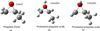 |
Fig. 1 Structure of propylene oxide and two of its protonated forms. |
Surface reactions for propylene and propylene oxide synthesis.
Kinetics of the reaction between C3H6 and O.
2 Reaction pathways
2.1 Methodology
To study the formation and destruction reactions of propylene oxide and associated species, we considered both gas phase and grain surface reactions. To study the reaction pathways, we employed quantum chemical methods. We carried out quantum chemical calculations to find out the reaction enthalpies of these gas/ice phase reactions. In Table 1, we summarize all the surface reactions considered for the formation of propylene and propyline oxide. In Table 2, we provide the enthalpy of reactions between C3H6 and O(3 P) for five (R12-R16) product channels. The Gaussian 09 program was used (Frisch et al. 2015) for such calculations. In this work, we used the density functional theorem (DFT) with 6-311G basis set with the inclusion of diffuse (++) along with polarization functions (d,p) and B3LYP functional (Becke 1988; Lee et al. 1988). We used the polarizable continuum model using the integral equation formalism variant with the default self-consistent reaction field method (SCRF) to model the solvation-effect for the computation of enthalpy of the ice phase reactions.
2.2 Formation pathways
Marcelino et al. (2007) discovered propylene (C3H6) toward the TMC-1 by using the IRAM 30 m radio telescope. These authors estimated the column density of propylene ~ 4 × 1013 cm −2. Herbst et al. (2010) studied the formation of gas phase propylene in the cold interstellar cloud. They proposed that propylene could mainly be formed by the dissociative recombination (DR) of its precursor ion,  via
via 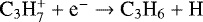 . For the formation of
  , the following reactions were included in the UMIST 2012 (McElroy et al. 2013) network:
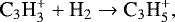
But a recent study by Lin et al. (2013) found that above two reactions contain some activation barrier (25.5 and 24.7 kJ mol−1, respectively). In the low-temperature regime, it is problematic to overcome such a high barrier in the gas phase and thus the formation of gas phase  is inadequate by these routes; this suggests considering some alternative reaction pathways to enable the formation of C3H6 rather than by the electron recombination reaction as proposed by Herbst et al. (2010). Recently, Hickson et al. (2016) proposed some pathways for the formation of C3H6 in the ice phase. In this work, we also considered their pathways for the formation of this species. In Table 1, we list the formation and destruction pathways of C3H6 found in the literature and calculated in this work. Though we considered the formation of C3 on the grain surface, around the low temperature, its formation on the grain surface is not adequate owing to the higher binding energy (4000 K from the KIDA database) of the C atom. C3 is efficiently forming on the gas phase and thus the formation of C3H6 begins after the accretion of gas phase C3 on the grain surface. Sequential hydrogenation reactions (R1-R8 of Table 1) in the ice phase then leads to the formation of C3H6. Most of these hydrogenation reactions are barrierless (only reaction R6 has some barrier), so these pathways are very efficient for the formation of C3H6 in ice phase. Recently, Bergantini et al. (2018) used the reaction between CH and C2H6 for the formation of propylene with a branching fraction of 0.25 (R18). We also considered reaction numbers R18 and R19 (0.75 branching fraction) of Table 1 in our calculations. A high abundance of ice phase species may be reflected in the gas phase by various efficient desorption mechanisms such as thermal, nonthermal, and cosmic-ray-induced desorption.
The gas phase reaction between oxygen atom O(3P) and propylene (C3H6) has been well studied by several authors (Stuhl & Niki 1971; Atkinson & Cvetanov 1972; Atkinson & Pitts 1974; Knya et al. 1992). The branching ratios of the reaction between C3H6 and O atom were studied by DeBoer & Dodd (2007). They showed that the propylene and oxygen atom could form a stable biradical (CH3CHCH2O) having an activation barrier of ~ 7.5 kJ mol−1. Dissociation of this biradical follows various pathways with both singlet and triplet potential energy surfaces. Isomerization of PrO can produce (a) acetone, (b) propanal (c) methyl vinyl alcohol, and (d) ally alcohol. However, all these have to overcome very high activation barriers (Dubnikova & Lifshitz 2000), which is not possible at our desired environment.
Ward &Price (2011) described the production of EO and PrO on interstellar dust (graphite surface). They found an activation barrier of about 40 K for the formation of PrO by the reaction between C3H6 and O(3 P). Hudson et al. (2017) proposed that the reaction between O(3P) atom and C3H6 can produce any of the following five species, namely, (i) propylene oxide (C3H6O), (ii) propanol (CH3CH2CHO), (iii) 1-methyl vinyl alcohol (CH3COHCH2), (iv) acetone (CH3COCH3), and (v) 2-methyl vinyl alcohol (CH3CHCHOH). We carried out quantum chemical calculations to find out the reaction enthalpies of these gas/ice phase reactions. In Table 2, we show the enthalpy of reactions between C3H6 and O(3 P) for these five (R12-R16) product channels. Table 2 depicts that in between the five product channels (R12-R16), the production of acetone is comparatively most favorable and the production of PrO is least favorable. In Table 1, reactions R12-R16 are arranged according to their exothermicity values obtained from our calculated values in Table 2. Ward & Price (2011) found an activation barrier of about 40 K for the formation ofice phase PrO. We considered the activation barrier of the other product channels using a scaling factor based on their exothermicity values obtained from the ice phase reactions of Table 2. The ice phase rate coefficients of these reactions (R12-R16) were calculated by the method described in Hasegawa et al. (1992), which is based on thermal diffusion. For the binding energy of O, we used 1660 K (He et al. 2015)and for C3H6 we used 2580 K (Ward & Price 2011), respectively. For the other species, we considered the most updated set of energy barriers available in KIDA database. Calculated ice phase rates for these five product channels are shown in the last column of Table 2 for (Tice = 25 K).
Recently Leonori et al. (2015) computed the rate constant for the formation of gas phase PrO at high temperature for the addition and abstraction reactions interpolated between 300−2000 K. According to their results, formation of PrO by the addition of C3H6 and O(3P) can be approximated by the following Arrhenius expression:

where α = 4.52 × 10⁻¹⁶, β = 1.406 and Ea, the activation barrier is − 12.5 K. We assumed that this reaction is also feasible around the low temperature as well. Using the above relation, at 30 K, we have a rate of 8.3 × 10⁻¹⁴ cm3 s−1 for the formation of gas phase PrO (R16 of Table 2). Since the activation barrier for the other four products resulting from the gas phase reaction between C3H6 and O (R12-R15 of Table 2) are yet to be known, we used their gas phase exothermicity values pointed out in Table 2 to scale the activation barrier (Ea). Thus, for these four product channels, we have kept α and β same as the gas phase reaction number R16 of Table 2 and have scaled Ea according to their exothermicity values.
Dickens et al. (1997) proposed the following gas phase formation pathways of EO:

followedby

Following the same trend as EO, we also assumed that all the isomers of PrO could also be produced by the DR of C3H7O+ with the same rate. The formation of C3H7O+ ( ; i.e., protonated acetone or ethyl, 1- methoxy-, ion) was already included in the UMIST 2012 network, so we did not use any additional channel to form this ion. Instead, only the destruction of this ion by the DR is considered.
2.3 Formation by suprathermal oxygen
Recently, Bergantini et al. (2018) carried out a combined theoretical and experimental work to study the formation of interstellar PrO. They found that the galactic, cosmic-ray-induced ice phase chemistry with suprathermal oxygen (O* or O(1 D)) may lead to the significant amount of PrO (R17 of Table 1). For the generation of suprathermal oxygen, they considered the dissociation of CO2, H2O, and CO. The rate constants of the radiolysis were calculated using the following relation:
![Mathematical equation: \begin{equation*} R=\frac{\zeta}{10^{-17} [\textrm{s}^{-1}]} \frac{G}{100 [\textrm{eV}]}S_{\textrm{e}} \phi_{\textrm{ism}} \ \ \ \textrm{s}^{-1}, \end{equation*}](/articles/aa/full_html/2019/08/aa34923-18/aa34923-18-eq11.png)
where, G is the radiolysis yield per 100 eV, Se is the electronic stopping cross section, Φism is the interstellar cosmic-ray flux and ζ is the cosmic-ray ionization rate. We used same G value as used in Bergantini et al. (2018) (2.23, 0.7, and 0.8 for CO2, H2O, and CO, respectively), ϕism = 10 cm−2 s−1 following Abplanalp et al. (2016). We used ζ = 1.3 × 10⁻¹⁷ s−1 instead of 1.3 × 10⁻¹⁶ used in Bergantini et al. (2018). Although Abplanalp et al. (2016) mentioned that Se is the electron stopping cross section for electrons, Bergantini et al. (2018) used Se as the electron stopping cross section for protons from the PSTAR program1. We used ESTAR program2 as used by Abplanalp et al. (2016) for the computation of the Se parameter. Since, Se is sensitive to the projectile energy, for a better approximation for Se, we used projectile energy of the electron 1 KeV (minimum available value in the ESTAR program), 5 KeV, and 10 KeV, respectively, and considered their average. We found Se = 3.62 × 10⁻¹⁵, 1.80 × 10⁻¹⁵, and 2.34 × 10⁻¹⁵ ev cm2 molecule−1 when we used CO2, H2O, and CO ice as target materials, respectively. For the density of the target materials, we used 1.3, 1, and 0.81 gm cm−3 for CO2, H2O, and CO ice,respectively, from Lauck et al. (2015) and references therein. By considering these Se parameters, we obtained rate constants of 1.05 × 10⁻¹³, 1.64× 10⁻¹⁴, and 2.43× 10⁻¹⁴ s−1 for CO2, H2O, and CO ice, respectively, as a target material.
For the consideration of the suprathermal oxygen (O(1D)) in our network, we considered some trivial approximations. After the generation of these suprathermal oxygens, they are treated similarly as the O(3 P), except the reaction with C3H6. For the reaction between C3H6 and O(1D), we assumed that the reaction is barrierless in nature and process in each encounter. The binding energy of the O(1 D) is assumed to be the same as O(3P) and supposed to behave similarly in the gas phase upon its sublimation. We did not consider the O(1 D) insertion reactions for any other species in our network. We used these reactions only for the formation of PrO. We tested the effect of these oxygen insertion reactions on the abundances of the major species, which remain mostly unaltered.
2.4 Destruction pathways
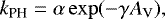
All the destruction pathways for the PrO along with its isomers are shown in Table 3. We considered IN reactions for the destruction of PrO and its isomers. The most abundant ions like,  and HCO+ have been considered (Occhiogrosso et al. 2012). Additionally, DR, photodissociation (PH), and dissociation by cosmic rays (CRPH) have also been considered for the destruction. Ion-neutral reactions are very efficient for the destruction of neutral interstellar species. If the neutral species is nonpolar, we used the Langevin collision rate coefficient (Herbst 2006; Wakelam et al. 2010) and if the neutral species is polar, then we employed the trajectory scaling relation (Su & Chesnavich 1982; Woon & Herbst 2009). For the destruction by photoreactions, we used the following equation:
 (1)
(1)
where α is the rate coefficient (s−1) in the unshielded interstellar ultraviolet radiation field, AV is the visual extinction, and γ controls the extinction of the dust at the ultraviolet wavelength. We used α = 1.13 × 10−09 s−1 and γ = 1.6 for the PH of CH3CHCH2.
For the cosmic-ray-induced photoreactions, we used the following relation (Gredel et al. 1989):
 (2)
(2)
where, α is the cosmic-ray ionization rate (s−1), γ′ is the number of photodissociative events that take place per cosmic-ray ionization and ω is the dust grain albedo in the far ultraviolet. We used ω = 0.6, α =1.3 × 10⁻¹⁷ s−1, and γ′ = 750.0 by following the cosmic-ray-induced photoreactions of CH3OH in Woodall et al. (2007).
3 Chemical modeling
We used our large gas-grain chemical network (Das et al. 2008b, 2013a,b, 2015a,b; Majumdar et al. 2014a,b; Gorai et al. 2017a,b) to estimate the formation of PrO in the star-forming region. The gas phase chemical network is mainly adopted from the UMIST 2012 database (McElroy et al. 2013) and the grain surface chemical network is primarily developed from Ruaud et al. (2016). As the initial elemental abundances (Table 4), we considered the “low metal” abundance with C/O ratio ~ 0.607 (Hincelin et al. 2011), which are often used for the modeling of dense clouds, where the majority of the hydrogen atoms are locked in the form of hydrogen molecules.
3.1 Dark cloud model
3.1.1 Physical condition
To mimic the observed region of the PrO, we considered a total hydrogen number density (nH) = 2 × 104 cm−3 and a gas temperature (Tgas) = 30 K and dust temperature (Tice) = 10 and 25 K, respectively. We assumed a visual extinction parameter (AV) of 30 and considered a cosmic-ray ionization rate (ζ) of 1.3 × 10⁻¹⁷ s−1 (Herbst & Klemperer 1973). Since reactive desorption (Garrod et al. 2007) is a very efficient means to transfer surface species into the gas phase upon formation, we considered this in our model.
3.1.2 Results and discussions
Chemical evolution of PrO and C3H6 is shown in Fig. 2. The left panel of Fig. 2 is for Tice = 10 K and right panel is for Tice = 25 K. The left panel depicts two scenarios: one scenario has a fiducial reactive desorption parameter of a = 0.03 and the other has that of a = 0; unless otherwise stated, we always used this value (a = 0.03) of desorption factor along with the desorption probability 1 (for the reactions producing single product). This shows that when reactive desorption parameter is absent (a = 0), the formation of PrO is insignificant in both the phases. The reason for this is that C3H6 can efficiently be formed on ice phase but when a = 0.03 is considered, a significant portion of C3H6 can be able to transfer to the gas phase, which is not possible for a = 0. Woodall et al. (2007) considered barrierless reactions for the formation of  and
and  in gas phase. But it is already discussed in Sect. 2.2 that these two reactions contain high barrier and it is quite problematic to overcome such a high obstacle around low temperature. Moreover, because of high-energy barrier of O atom (1660 K for ground-state oxygen and suprathermal oxygen atom), oxygenation reaction is not as fast as hydrogenation reaction at low temperatures (Tice = 10 K) and thus the ice phase PrO formation is inadequate at low temperatures. At low temperatures (~ 10 K) PrO can mainly be formed in the gas phase bythe reaction between O atom and C3H6, where the major contribution of C3H6 is coming from the ice. As we increased the temperature (right panel, Tice = 25 K), the situation has changed because of the increase in the mobility of O atom on grain, which enables a significant production of PrO on the grain surface. From our dark cloud model (for a = 0.03 and Tice = 10 K), in between our simulation timescale (~106 yr), we have a peak abundance (w.r.t. H2) of PrO to be 4.17 × 10⁻¹⁴ and 5.26 × 10⁻¹⁴ in the gas and ice phases, respectively, whereas for a = 0.03 and Tice = 25 K it is 1.33 × 10⁻¹¹ and 2.04 × 10⁻⁷, respectively. In order to check the dependency of our result on the fiducial factor, we further considered a = 0.01 and Tice = 25 K and found that the peak gas phase abundance (~4.58 × 10⁻¹²) decreased by ~3 times compared to the case with a = 0.03 and Tice = 25 K.
Since, the abundance of C3H6 in the gas phase is not adequate, no significant amount of PrO is obtained for Tice = 10 K but for Tice = 25 K, formation of C3H6 significantly enhanced and resulting significant increase in the production of PrO. To find out a parameter space for the formation of PrO in the dark cloud condition, we varied the number density of total hydrogen (nH) in between 104 and 107 cm−3 and ice temperature between 10 and 25 K and kept the gas temperature at 30 K. The resulting plot is shown in Fig. 3. It is clear from the plot that the observed abundance (approximately × 10−11) of PrO can be obtained in between nH = 104−105 cm−3 and the ice temperature range from 20 to 25 K.
Since we considered a small activation barrier of about 40 K for the ice phase reaction between C3H6 and O(3 P), consideration of suprathermal oxygen has not influenced our results. It is important to keep in mind that because of the unavailability of the binding energy values for O(1 D), we considered the same binding energy as that for O(3P). However, it is expected that because of the generation process of the suprathermal oxygen, it would carry some extra energy which would enable it to move much faster than O(3 P). Thus, it is expected that the binding energy of O(1D) would be lower than O(3P). We tested the abundance of PrO again by considering a lower binding energy value (half of the normal oxygen) for O(1 D). However, again for this case, we did not find any significant difference. The reason behind is that, on the one hand, lower binding energy provides much faster diffusion rate and enhances the chance of recombination, but on the other hand, it gives much quicker sublimation rate. This decreases the residence time of O(1 D) on the grain surface and thus reduces the chance of recombination. Since in our network, PrO mainly formed by the reaction between C3H6 and O(3 P), lowering the binding energy of O(1D) did not change our PrO abundance. A higher dose of cosmic rays would be useful to generate more suprathermal oxygen; this could be helpful in the PrO formation, but it would also dissociate PrO as well. We think that the cosmic-ray ionization rate of about 1.3 × 10⁻¹⁷ s−1 used in this work is a standard value for the region in which the three transitions of PrO were observed.
Destruction pathways of PrO and its isomers.
Initial elemental abundances with respect to total hydrogen nuclei.
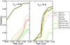 |
Fig. 2 Chemical evolution of PrO and C3H6 for a dark cloud model. The solid line represents ice phase abundance and dotted line represents the gas phase abundance. |
 |
Fig. 3 Parameter space of the abundance of PrO in dark cloud conditions. The color bar represents the fraction abundance of PrO. |
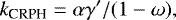
3.2 Hot core model
3.2.1 Physical condition
Cunningham et al. (2007) attempted to observe PrO and glycine in Sgr B2(LMH) and Orion-KL with the MOPRA Telescope. However, they did not detect either species but were able to put an upper limit on the abundances of these two molecules in these sources. They proposed an upper limit of about 6.7 × 1014 cm−2 for the column density of PrO in Sgr B2 (LMH). To estimate the abundance of PrO in the hot core region, we considered a two-phase model as used by Garrod & Herbst (2006). The first phase is assumed to be isothermal at 10 or 25 K and lasts for 106 yr. For this phase, we considered AV = 30 and ζ = 1.3 × 10⁻¹⁷ s−1. The subsequent phase is assumed to be a warm-up period where the temperature can gradually increase up to 200 K in 105 yr. So our total simulation time is restricted up to a total 1.1 × 10⁶ yr. The number density of the total hydrogen is assumed to be constant (nH = 104−107 cm−3) in both phases of our simulation.
3.2.2 Results and discussions
In Fig. 4, we show the chemical evolution of PrO for various density clouds (nH= 104−107 cm−3). The last panel shows the abundance variation of peak gas phase abundance and final abundance (i.e., at the end of the simulation the timescale ~ 1.1 × 10⁶ yr) of PrO with the number density variation. In case of the Tice = 10 K, as we decreased the density, the gas phase abundance of PrO increased slightly and have a maximum (~ 1.5 × 10⁻⁷ w.r.t. H2) around nH = 1 × 104 cm−3. In the high-density region (~ 107 cm−3), we obtained the peak abundance ~1.3 × 10⁻⁹. The final abundance for this case varies between 1.4 × 10⁻¹⁰ and 8.9 × 10⁻⁸. In case of Tice = 25 K, the peak and final abundance roughly remain invariant; the peak abundance varies between 1.03× 10⁻⁷ and 2.4 × 10⁻⁷ and final abundance varies between 1.7 × 10⁻⁸ and 3.5 × 10⁻⁸.
3.3 Comparison with the previous modeling results
There are some basic differences between the model described above and those used by the other authors to explain the observed abundance of PrO. Recently, Bergantini et al. (2018) have used a combined experimental and theoretical study to explain the abundance of PrO in the ISM. They have explained the formation of PrO by nonequilibrium reactions initiated by the effects of secondary electrons. More specifically, they used suprathermal (1 D) oxygen insertion reaction with propylene to explain the PrO formation. They did not consider the formation of PrO by the addition of ground state oxygen (3P). In our case, we considered the formation of PrO by both types of oxygen atoms. Ward & Price (2011) found a low activation barrier (~ 40K) for the ice phase reaction between C3H6 and O(3P). Such a low activation barrier could be overcome at low temperatures. As a result, we found an adequate production of PrO even in absence of the suprathermal oxygen insertion reaction.
4 Vibrational spectroscopy
4.1 Methodology
To compute the vibrational transitions of PrO and its protonated form, we used the Gaussian 09 program. We used the DFT with 6-311G basis set including diffuse and polarization functions for these calculations. Initially, we verified our results with various methods and basis sets and compared it with the experimentally obtained results. We found that B3LYP/6-311++G(d, p) method is best suited to reproduce the experimentally obtained transitions of PrO. Moreover, we also considered IEPCM model with the method mentioned above to compute the vibrational transitions of PrO in the ice phase. All optimized geometry was verified by harmonic frequency analysis (having no negative frequency). We performed our calculations by placing the solute (species) in the cavity within the solvent (water molecule) reaction field. We used the SCRF method following the earlier study of Woon (2002).
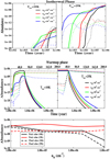 |
Fig. 4 Chemical evolution of PrO in a two-phase model by considering various cloud densities. The upper two panels indicate the isothermal phase, the middle two panels indicate the warm-up, and the lower panel is for the gas phase peak abundance of PrO and final abundance of PrO at the warm-up phase for various density cloud. Different colors denote different cloud densities. In the upper and middle panels, the solid line represents the abundance in the gas phase whereas the dotted line represents the abundance in ice phase. |
4.2 Results and discussions
In Table 5, we summarized calculated and experimental vibrational frequencies of PrO along with the integral absorption coefficients and band assignments. Similarly, Table 6 presents the determined vibrational frequencies along with the integral absorption coefficient of protonated PrO. Our calculated values of absorption coefficients and vibrational frequencies are in excellent agreement with the experimentally obtained results (Hudson et al. 2017). Puzzarini et al. (2014) studied the spectroscopic details of protonated oxirane (C2H5O+). Similarly, protonation of PrO can take place. PrO could be protonated via IN reactions in which the proton is transferred to the neutral. Protonated PrO may be formed in the gas phase by the reaction of PrO with the ions such as H3O+, HCO+, and  . We found a proton affinity of PrO about 803.169 kJ mol−1 by doing quantum chemical calculations (using the HF/6-31G(d) method), which is in excellent agreement with Hunter & Lias (1998) (803.3 kJ mol−1). For anotherprotonated form of PrO, the proton affinity value is found to be 801.827 kJ mol−1. Thus, the protonated PrO shown in Fig. 1c possesses slightly higher energy (about 175 K) than protonated PrO shown in Fig. 1b. Since the experimental data for protonated PrO are yet to be published based on the accuracy obtained for the vibrational transitions of PrO, the same method and basis set were applied for protonated PrO to compute the vibrational transitions and integral absorption coefficients. Panels a and b of Fig. 5 depict the absorption spectra of PrO and its protonated form. Figure 5a covers 1600 − 200 cm−1 region (some parts of the mid-IR: 2000−400 cm−1 and some parts of the far-IR: 400−50 cm−1) and Fig. 5b covers 3800−3000 cm−1 region (i.e., some parts of the near-IR: 12 800−2000 cm−1).
Vibrational analysis of propylene oxide using B3LYP/6-311++G(d,p).
Vibrational analysis of protonated propylene oxide (C3H6OH+) using B3LYP/6-311++G(d,p).
4.3 Comparison with experimentally obtained results
In the upper and lower panels of Fig. 6a, a comparison between our computed and experimentally obtained vibrational spectra is shown for (1600−800) cm−1 and (3200−2700) cm−1 frequency window, respectively. In these two panels, we also show how the clustering of PrO can affect the computed vibrational spectra of PrO. The blue line in Fig. 6 represents the experimental data extracted from Hudson et al. (2017), whereas the black, red, and green lines represent the calculated spectra with PrO monomer, PrO dimer, and PrO tetramer, respectively. Figure 6a depicts that in the mid-IR region, we have a good agreement between our theoretical and experimental results of Hudson et al. (2017). We noticed that most of the transitions within this mid-IR region are within an error bar of about 10 cm−1. One transition at 1291.89 cm−1 is found to be shifted maximum by 25 cm−1. The intensity of each mode of vibration and the area under the curve of various regime changes with the cluster size of PrO. We noticed that if a scaling factor of 0.9728 is used, there is an excellent agreement around the stretching mode, and thus in Fig. 6b we scaled our computed wavenumber accordingly.
5 Radiative transfer modeling
5.1 Methodology
In astrochemistry, a major aim of radiative transfer modeling is to extract the molecular abundances from the line spectra at infrared andsub(millimeter) wavelengths. Three different levels of radiative transfer model are in use, which range from the basic local thermodynamic equilibrium (LTE) models to complex nonlocal models in 2D and even more complex models in 3D (Van der Tak 2011).
A simple single excitation temperature model, i.e., LTE modeling was carried out to predict the most probable transition of PrO. We consider LTE modeling to be a good starting point for predicting the line parameters around the high-density region. Moreover, itdoes not require additional collisional information. We used the CASSIS program, which was developed by IRAP-UPS/CNRS3 for the LTE modeling. Recently, McGuire et al. (2016) observed three transitions of PrO in absorption. Cunningham et al. (2007) used the MOPRA telescope at the 3 mm band for theidentification of various transitions of PrO in Sgr B2(LMH) and Orion-KL. They were unable to detect any PrO transitions in these two targeted regions but they had provided an upper limit for the abundance of PrO around these sources. We carried out the LTE calculations for two different cases. The first is for the sources in which we are expecting the transitions of PrO in the extended molecular shell around the embedded, massive protostellar object as observed by McGuire et al. (2016) and for the second, we considered the input parameters in such a way that wemay observe some strong transitions of PrO in the hot core regions as attempted by Cunningham et al. (2007).
In the LTE model, level populations are controlled by Boltzmann distribution. As an interstellar chemical process that is far from thermodynamic equilibrium, it is essential to consider the non-LTE method in which the balance between the excitation and de-excitation of molecular energy levels are explicitly solved. Both the collisional and radiative processes contribute to this balance. Most importantly, for the non-LTE method, the collisional data file is required that is not available for most of the species. Collisional data file for PrO was not available in any database. To have an educated estimation of the line parameters in non-LTE, we considered the collisional rate parameters of e-CH3OH with H2 (Rabli & Flower 2010) for preparing the collisional data file of PrO. Since PrO is a slightly asymmetric rotor molecule, it would have been better if we used the collisional parameters of H2CO in this work. But the unavailability of the collisional rates for the sufficient number of energy levels for H2CO tempted us to use e-CH3OH as an approximation for which we have the collisional parameters available in LAMDA database (Schöier et al. 2005) for sufficient number of energy levels. We used the RADEX program (Van der Tak et al. 2007) for this non-LTE computation.
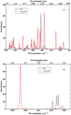 |
Fig. 5 Comparison between our calculated IR spectra of propylene oxide and protonated propylene oxide. |
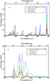 |
Fig. 6 Comparison between our calculated spectra with those obtained in the experiment (Hudson et al. 2017). The results of Hudson et al. (2017) have been digitally extracted using https://apps.automeris.io/wpd. Upper panel: the mid-IR region. Lower panel: the near-IR region. For the sake of better visualization, we scaled down the Y-axis of our calculated values in (a) and (b). Our calculated wavenumber in the X-axis of (b) is scaled by 0.9728 to have better agreement. |
5.2 Results and discussions
5.2.1 LTE model
For the first case, we considered the GBT 100 m telescopic parameter for the modeling and adopted parameters are shown in Table 7. For this case, we assumed that the source size (θs) 20″ and beam size (θb) may vary depending upon the frequency by  (Hollis et al. 2007), where ν is the frequency in GHz. Beam dilution factor is computed by
  and applied on the obtained intensity. The recent observation by McGuire et al. (2016) observed three transitions of PrO in cold molecular shell in front of the bright continuum sources/hot cores within Sgr B2. In Table 8, we point out the obtained LTE parameters for these three transitions only. We noticed that the obtained intensities are very weak and are even below the RMS noise level of 1 mK. The reason behind this result is that in the CASSIS module of LTE we used a constant background continuum temperature of 2.73 K. However, a variable background continuum temperature was required to observe these transitions in absorption. We return to the discussion about the absorption feature of these three transitions in a later section of this paper.
For the second case, we modeled the LTE transitions of PrO for the hot core region. We used our computed gas phase PrO abundance ~ 1.74 × 10⁻⁸ (final abundance with nH = 106 cm−3 or  cm−3 with initial dust temperature 25 K). We used theAtacama Large Millimeter/submillimeter Array (ALMA) 400 m telescopic parameter to model this feature. We considered that source size (1.5″) and beam size vary as
  (for ALMA 400 m) and the beam dilution effect applied following the same formula (
 ) mentioned above. To verify the potential observability of these PrO transitions, we checked the blending of these transitions with any other interstellar molecular transitions. Interestingly, we identified a few intense transitions of PrO in Band 3 (84−116 GHz) and Band 4 (125−163 GHz) which are not blended. In Table 9, we point out all the potentially observable transitions of PrO in the hot core region. Based on our simple LTE model, we isolated some strong transitions of PrO. We further used the ALMA simulator to check the integration time required to observe these transitions by ALMA. We found that for ALMA Band 4 (for e.g 130 GHz), with 20 mK RMS noise, 0.4 km s−1 spectral resolution, and 43 antennas along with the dual polarization, 1 hr on-source integration time is required for 5σ detection of PrO in Sgr B2 (N) with an angular resolution of 1.5″. For the similar configuration, 3 h on-source integration time is required for a Band 3 (e.g., 100 GHz) observation with ALMA.
Input parameters used for the LTE modeling.
LTE line parameters of the various transitions of PrO using GBT.
LTE line parameters of the various transitions of PrO using ALMA.
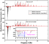 |
Fig. 7 Line parameters of PrO for non-LTE condition by considering (a) constant source size (20”) and (b) varied source size (Hollis et al. 2007). The observed and other possible transitions are highlighted inside a separate box in Fig. 7. |
5.2.2 Non-LTE
In panels a and b of Fig. 7, we show our computed radiation temperature for the various transitions of PrO within a wide range of frequency (1−200 GHz). In this case, our target was to find out the line parameters that are relevant for the observations performed by McGuire et al. (2016). Thus, we considered, Tex= 5 K, a column density of PrO = 1 × 1013 cm−2, a FWHM = 15 Km s−1 (for the observed three transitions, McGuire et al. 2016 obtained a full width at half maximum (FWHM) of 11.6, 15.8, and 19.6, respectively, and we considered the average of these three FWHMs) and  cm−3. For this non-LTE model, we used GBT 100 m telescopic parameters. Background continuum temperature measurement was already carried out by Hollis et al. (2007). These authors showed the observed continuum antenna temperatures by the GBT spectrometer toward SgrB2 (N-LMH). We considered this variation of background temperature by digitally extracting Fig. 1 of Hollis et al. (2007) using an online programme4. For the GBT 100 m telescope, the changes in continuum temperature beyond 40 GHz are very small5. Extracting the values from Hollis et al. (2007), we have the continuum temperature ~ 3.35 K at 49 GHz. Beyond this, they did not provide any data for the continuum temperature, so we considered a fixed continuum temperature of about 2.73 K beyond 100 GHz. In between the 49 and 100 GHz we interpolated the continuum temperature from 3.35 to 2.73 K. We considered the variation of beam size by considering the relation
  (Hollis et al. 2007). In Fig. 7a, we considered that the source size is constant at 20″ and in Fig. 7b, we considered the source size variation using
  (Hollis et al. 2007). We present the radiation temperatures of the various transitions of PrO in Fig. 7a and b, considering the beam dilution effect and avoiding this effect. Most interestingly, with the given conditions, we obtained all the three transitions (12.07, 12.8, and 14.04 GHz) in absorptions. Additionally, we identified three more transitions at 15.78 GHz, 18.1 GHz, and 23.98 GHz, which might potentially be observed around the same region where the other three transitions were observed.
We further worked on these six transitions to find out the region that shows the absorption feature. In this effort, we used a wide range of parameter spaces (by varying the number density and kinetic temperature of the medium) to find out the probable absorption zone for these transitions. We used the RADEX program again for this purpose. In Fig. 8, we show the variation of the radiation temperature depending on the H2 density (104 −107 cm−3) and kinetic temperature (5−35 K). This figure depicts that the absorptions are prominent around the low kinetic temperature (5− 10 K) and for  cm−3. The value of the color box at the end of the panels represents the obtained radiation temperature of the transitions in K.
In addition to the three transition of PrO discussed above, McGuire et al. (2016) observed 18 transitions of acetone and 11 transitions of propanal from the Prebiotic Interstellar Molecular Survey (PRIMOS). To test the fate of these transitions with the collisional rate file adopted from e-CH3OH, we calculated the radiation temperature of these transitions for a wide range of parameter spaces. We further explored the validity of our collisional data file by checking the computed radiation temperature of propanal and acetone in PRIMOS. In Figs. A.1 and A.2, we show the radiation temperature of 11 transitions of propanal and 18 transitions of acetone that were observed in PRIMOS. Figure A.1 shows that for the first six transitions of propanal, we obtained the absorption feature at Tex= 5−7 K and relatively at higher densities ( cm−3). For the transitions at 29.619 and 31.002 GHz, we obtained the absorption features at relatively lower H2 densities (103 −104 cm−3) and kinetic temperatures (10−35 K). We noticed that the last three transitions of propanal show emission for the whole range of density and temperature adopted in this work. Similarly in case of Fig. A.2, for the first 14 transitions of acetone, we obtained the absorption feature within a minimal zone of parameter space, but for the last four transitions we did not receive the absorption feature. Since then we saw a significant discrepancy between our calculated and observed radiation temperature at the higher frequencies, which could be attributed to the unavailability of the collisional rates and its present approximation.
Our non-LTE model accurately reproduces the three observed transitions of PrO in absorption, and for this, we used observed parameters such as excitation temperature, FWHM, and column density of PrO following McGuire et al. (2016). We also found a good agreement between the observed transitions of propanal and acetone with our calculated non-LTE transitions. The parameter spaces for the radiation temperature of the most probable transitions of PrO, propanal, and acetone are presented (Figs. 8, A.1 and A.2) with the non-LTE condition. Similar results obtained by observation (McGuire et al. 2016) and radiative transfer model are used to constrain the physical conditions (density, temperature) of the region in which these molecules were observed.
In Table 9, we already pointed out the line parameters of various PrO transitions for the hot core region that lies in the ALMA Band 3 and Band 4 regions. For all the transitions shown in Table 9. we show the variations of radiation temperatures in Fig. A.3 for a wide range of parameter spaces. In constructing the parameter space for the hot core region, we used Tex = 5−160 K and  cm−3. Outside each panel, a color box is placed to show the radiation temperature in K. Figure A.3 gives information that is very useful to gain an understanding of the emission feature of these viable transitions before its real observation.
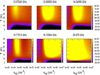 |
Fig. 8 Parameter space for the radiation temperature of the most probable 6 transitions with non-LTE condition. |
5.3 Estimation of physical properties from obtained line parameters
Mangum & Wootten (1993) used a formaldehyde (H2CO) molecule to trace kinetic temperature and spatial density within molecular clouds. Normally, symmetric rotor molecules (e.g., NH3, CH3CN, and CH3C2H) are used for the measurements of kinetic temperature. However, the usage of these species are doubtful because of the spatially variable abundances and complex excitation properties. The main reason behind the choice of formaldehyde was that it permeates the ISM at a relatively high abundance. Formaldehyde is a slightly asymmetric rotor molecule that should possess closer kinetic temperaturesensitivities such as purely symmetric rotors. Since PrO is an asymmetric top molecule, the ratio of lines from different J states would be used as the density tracers and the ratio of lines from the same J state but different K-states could be used as probes of the regional temperature.
5.3.1 Kinetic temperature measurements
In the case of symmetric rotors, ΔKa = 0 dictates the dipole selection rules. Transitions between other Ka values are only possible by the collisional excitation. Owing to this unique feature, a comparison between the energy level populations from different Ka levels withinthe same symmetry species may be used as a measure of the kinetic temperature. If we consider the ratio between two transitions that could be measured within the same frequency band, various observational uncertainties could be nullified.
Propylene oxide is an asymmetric rotor. We can check the line ratio of propylene oxide for the measurement of temperature and check the consistency of this method with that obtained for H2CO. Figure 9 depicts the rotational energy level diagram of propylene oxide. Because of its complexity, PrO is not as widespread as H2CO. On the other hand, PrO is also a slightly asymmetric top molecule, and thus we can compare the line ratios obtained by the PrO observation with the H2CO observation to derive the precise kinetic temperature of the source. The collisions primarily connect different Ka ladders of PrO. Thus the relative population occupying the ground states of these two Ka ladders are related by the Boltzmann equation at Kinetic temperature. Based on the selection process of Mangum & Wootten (1993) for the measurement of the kinetic temperature, we used the following selection rule to have the line ratio between twotransitions. Suppose the line ratio (R) between the two transitions is
where, Ji, Ka i, Kc i (i = 1, 4) are used to denote the quantum numbers of the energy levels involved in the transition. We used the following selection rules for the measurement of the kinetic temperature from the line ratio: (a) ΔJ = 1 (i.e., J1 − J2 = J3 − J4 = 1), (b) J1 = J3 and J2 = J4, (c) ΔKa = 0 (i.e., Ka1 − Ka2 = Ka3 − Ka4 = 0), (d) Ka1≠Ka3, Ka1≠Ka4, Ka2≠Ka3, Ka2≠Ka4, (e) ΔKc = 1 (i.e., Kc1 − Kc2 = Kc3 = Kc4 = 1), and (f) the frequency should be closely spaced. Unfortunately, the observed three transitions (McGuire et al. 2016) did not fulfill the above criterion. Thus, we are unable to predict the kinetic temperature from the line ratio method in this work. Alternatively, we focused on the transitions of PrO that might be observed in the hot core region and identified some of the transitions that might be useful to find out the physical properties of the perceived source. In Table 9, we already selected some transitions based on the obtained intensity and avoided blending with possible interstellar species. Among these, we found out some transitions for the measurement of the kinetic temperature. The advantage of plotting these line ratios are that these are less sensitive to the calibration errors and both the lines would have been equally affected. It is worthy to calculate several transition ratios to avoid the discrepancy in measuring the kinetic temperature. We found out following line pairs for the measurement of the kinetic temperature:  . The line ratios of PrO mentioned in this work have the transitions from various Ka ladders (i.e., with the Ka = 3, 4, 5, 6, 7, 8, 9). It is obvious that around the low-temperature region, the ground state of the Ka ladders are well populated and lower Ka values would pile up earlier than those of the higher Ka values.
From Fig. 9, the ground state of Ka = 3, 4, 5, 6, 7, 8, and 9 ladder is 331, 441, 551, 661, 771, 881, and 991, respectively.The upstate energy of the each transitions considered are all below 100 K. Let us first check under LTE approximation how these ratios can behave. At the high densities, LTE conditions are best suited. Therefore, the relative population occupying the ground states from the two Ka ladders should obey the Boltzmann equation at the kinetic temperature. Mangum & Wootten (1993) derived the following relation for the estimation of kinetic temperature from the obtained line ratio if both the transitions are optically thin:
![Mathematical equation: \begin{equation*} T_{\textrm{K}}=[E(J,K')-E(J,K)]\left[\textrm{ln}\left(\frac{S_{JK'}\int J(T_{\textrm{R}}(J,K)\textrm{d}\nu}{S_{JK}\int J(T_{\textrm{R}}(J,K')\textrm{d}\nu}\right)\right]^{-1},\end{equation*}](/articles/aa/full_html/2019/08/aa34923-18/aa34923-18-eq31.png) (3)
(3)
where, E(J, K′) is the upstate energy of the bottom transition, E(J, K) is the upstate energy of the transition at the numerator,  and SJK are the transition line strengths of the two upstate involved in the transition ratio, and TR (J, K′), TR (J, K) are the obtained radiation temperatures. By using the above relation and using the line strengths available6, we computed the line ratio of the radiation temperature for the above transitions. Figure 10 shows the variation of these line ratios with the various kinetic temperatures. It is interesting to note that around the low temperature, this ratio is maximum and drastically reduced with increasing temperature. After a certain temperature, it remains roughly invariant (small decreasing slope) on the increase of the kinetic temperature. This feature would be better understood if we explain it in terms of the 1st transition ratio,
  (see first panel of Fig. A.4). Around the low temperature (TK < 25.98 K) the ground state of the Ka = 3 (i.e., 331) and Ka = 4 ladder (i.e., 441) are mostly populated. Since 634 level lies below the 643 level, its population is comparatively higher at the low temperature. Similarly, 735 level lies below the 744 level and this implies that the population is higher in 735 level. As weincrease the temperature, the population at the ground state falls much faster. Since the upper and lower levels of the transition at the denominator are at a relatively higher energy levels than those of the upper and lower energy levels of the transition at the top, the population in the 643 level falls much faster than the 744 level and shows a faster increasing trend of 744−643 transition in comparison to the top transition. At TK > Eu the decreasing slope of the ratio changes and at TK ≫ Eu it tends to become roughly invariant on the kinetic temperature. The expression provided in Eq. (3) is independent of the number density of the cloud and thus provides the kinetic temperature at the LTE condition. Since we considered the hot core region, where the H2 density should be on the higher side (may vary in between ~ 105 and 107 cm−3) and temperatures should be between 100−200 K, the LTE condition is best suited. Since from various observations, we know the kinetic temperature of Sgr B2 (Bonfand et al. 2017), we may constrain the line ratio of PrO around this region. Our obtained line ratios from the LTE condition are presented in Table 10 at TK = 150 K.
Since we already prepared our approximated collisional rate file, we again calculated these line ratios with the non-LTE calculation for a wide range of parameter spaces. In our calculations, we varied the kinetic temperature from 5 to 160 K and kept the column density of PrO constant at 1013 cm−2. We also considered the column density as high as 1.74 × 1016 cm−2, which we obtained from our two-phase model presented in Fig. 4 and assuming a H2 column density of 1024 cm−2; in considering the column density, we see the effect on the calculated ratio but do not find any drastic difference. In Fig. A.4, we show the line ratios that might be useful to trace precisely the temperature of the region where these lines would be observed. At the top of the panel, we mentioned the upstate energy of four energy states that were involved in the transition ratio. In Table 10, we also note our line ratios obtained from the non-LTE calculations with nH = 107 cm−3 and Tex = 150 K. It should be noted that the line ratios obtained from the LTE calculation are uncertain by < 30% (Mangum &Wootten 1993) and we adopt random approximation for the consideration of our collisional data file. Despite this fact we obtained excellent agreement between the LTE consideration and non-LTE calculation (Table 10).
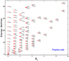 |
Fig. 9 Rotational energy level diagram of propylene oxide. |
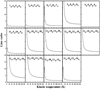 |
Fig. 10 Variation of line ratio with the kinetic temperature in LTE approximation. |
5.3.2 Spatial density measurements
Measurement of the spatial density is more critical than the measurement of the kinetic temperature. Based on the study by Mangum & Wootten (1993), spatial density could be measured by measuring a specific line ratio. Mangum & Wootten (1993) used the line ratio of various H2CO transitions for the measurement of the spatial density. We applied a similar technique to find out the line ratio for some of the observable transitions of PrO in the hot core region such as Sgr B2(LMH). We used the following criterion for the selection of the transition ratios: (a) ΔJ = 1 (i.e., J1 − J2 = J3 − J4 = 1), (b) J1≠ J3 and J2≠ J4, (c) ΔKa = 0 (i.e., Ka1 − Ka2 = Ka3 − Ka4 = 0), (d) Ka1 = Ka2 = Ka3 = Ka4, (e) ΔKc = 1 (i.e., Kc1 − Kc2 = Kc3 = Kc4 = 1), and (f) the frequency should be closely spaced. The above criteria are very rarely satisfied and sometimes the frequency lies very far away, and thus absolute calibration of each transition is required. The observed three transitions (McGuire et al. 2016) do not satisfy the above criterion. We also did not find any other transitions that can satisfy the above criterion around the region (dark cloud condition), where these three transitions were observed. Thus, we selected some more transitions (744− 643∕946 − 845, 744 − 643∕945 − 844, 744 − 642∕946 − 845, 743 − 642∕945 − 844, 827 − 726∕928 − 827) from the LTE model of the hot core region (Table 9), which can fulfill the above criterion and are suitable for observation in the hot core region. To constrain a limit on the number density, in Fig. A.5, we show the line ratios of the PrO transitions for Tex= 150 K. The parameter space is based on the column density of PrO and the H2 number density of the medium. The column densities are varied between 1013 and 1016 cm−2 and the H2 number density of the medium is varied between 104 and 107 cm−3. The density and temperature of the Sgr B2 (LMH) region were well studied, and it would be assumed that the H2 density may vary between 106 and 107 cm−3 and the kinetic temperature may vary between 100 and 150 K. Assuming the predicted upper limit of the PrO column density of 6.7 × 1014 cm−2 from Cunningham et al. (2007), we have the line ratio of 0.55, 0.57, 0.57, 0.59 and 0.8 for the above five transitions in the Sgr B2(LMH), respectively.
Estimated line ratio of PrO for the measurement of Kinetic temperature at 150K from LTE and non-LTE.
6 Conclusions
The presence of chiral species in the ISM been recently confirmed by McGuire et al. (2016). The observation of more chiral species and identification of their chirality may provide some insight into the homochirality of various pre-biotic species. In this paper, we studied the chemical evolution of PrO under various physical conditions and find out the line parameters of its transitions that are relevant to constrain the physical properties of the source. The major conclusions are the following:
A complete reaction network for the formation of PrO was prepared. This pathway is implemented in our gas-grain chemical model to find out its chemical evolution. To understand the formation of PrO in the cold environment as observed by (McGuire et al. 2016), we considered a static cloud model; for the formation of PrO in the hot core region, we considered a two-phase model, i.e., a static isothermal phase followed by a warm-up phase. We found that the reaction between C3H6 and O(3 P) with an activation barrier of 40 K is the dominant means for the formation of PrO in the ice phase. This ice phase PrO desorbed to the gas phase by various means that could be observed by their rotational transitions. We also considered the formation of PrO by O(1 D) but we noticed that we have significant production of PrO instead of this consideration. This is because of the lower activation barrier for the reaction between C3H6 and O(3P).
We computed various vibrational transitions of PrO along with its protonated form that might be observable with the forthcoming JWST facility.
To constrain the physical properties of the cloud, we carried out non-LTE modeling (by considering approximated collisional data file) for the most probable transitions identified by the LTE calculations by considering a wide range of parameter spaces (spanned by the H2 density range of ~ 103−107 cm−3 of the collisional partner and the kinetic temperature temperature range of ~ 5−35 K). We found that the observed three transitions at 12.07243 GHz (110 −101), 12.83734 GHz (211 −202), and 14.04776 GHz (312 −303) showed absorption features around the high H2 density (104 −107 cm−3) and low temperature (<10 K) region. Additionally, we found three more transitions (at 15.78, 18.10, and 23.975 GHz) that might be observed in absorption around the same region in which the three transitions were identified by McGuire et al. (2016).
We identified the line parameters suitable for the hot core observation of PrO. We point out potentially observable transitions lying in the ALMA Band 3 and Band 4, which would be used for the for future observations.
Various line ratios were directly found to be linked with the kinetic temperature and spatial density distribution. Thus from observation, we can extract the physical properties of the star-forming region by comparing their observation with our proposed parameters.
Our result depends on a very simple-minded cloud model that has no rotation; also the evolution was carried out until an estimated time. Thus the estimation of the parameters mentioned above could slightly depend on the evolution time inside the cloud. These aspects will be further explored in the future.
Acknowledgements
This research was possible in part due to a Grant-In-Aid from the Higher Education Department of the Government of West Bengal. A.D. is grateful to ISRO Respond project (Grant No. ISRO/RES/2/402/16-17). P.G. acknowledges the CSIR extended SRF fellowship (Grant No. 09/904 (0013) 2018 EMR-I). We want to acknowledge the reviewer for the numerous suggestions that improved the paper.
Appendix A Additional figures
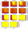 |
Fig. A.1 Parameter space for the radiation temperature of the 11 observed propanal transitions with non-LTE conditions. |
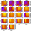 |
Fig. A.2 Parameter space for the radiation temperature of the 18 observed acetone transitions with non-LTE conditions. |
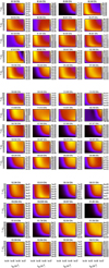 |
Fig. A.3 Parameter space of the radiation temperature for the probable PrO transitions in the hot core region. |
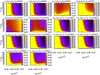 |
Fig. A.4 Variation of the line ratios (useful for the kinetic temperature measurement) for a wide range of parameter spaces (number density and kinetic temperature). |
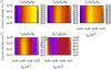 |
Fig. A.5 Variation of line ratios (useful for the measurement of the spatial density) for a wide range of parameter spaces (column density and number density). |
References
- Abplanalp, M. J., Förstel, M., & Kaiser, R. I. 2016, Chem. Phys. Lett., 644, 79 [NASA ADS] [CrossRef] [Google Scholar]
- Adams, F. C., Lada, C. J., & Shu, F. H. 1987, ApJ, 312, 788 [NASA ADS] [CrossRef] [Google Scholar]
- Agúndez, M., & Wakelam, V. 2013, Chem. Rev., 113, 8710 [CrossRef] [PubMed] [Google Scholar]
- Atkinson, R., & Cvetanov, R. J. 1972, J. Chem. Phys., 56, 432 [NASA ADS] [CrossRef] [Google Scholar]
- Atkinson, R., & Pitts, J. N. 1974, Chem. Phys. Lett., 27, 467 [NASA ADS] [CrossRef] [Google Scholar]
- Bailey, J., Chrysostomou, A., Hough, J. H. 1998, Science, 281, 672 [NASA ADS] [CrossRef] [Google Scholar]
- Bacmann, A., Taquet, V., Faure, A., Kahane, C., & Ceccarelli, C. 2012, A&A, 541, L12 [NASA ADS] [CrossRef] [EDP Sciences] [Google Scholar]
- Becke, A. D. 1988, Phys. Rev. A, 38, 3098 [Google Scholar]
- Bergner, J. B., Öberg, K. I., & Rajappan, M. 2017, ApJ, 845, 29 [NASA ADS] [CrossRef] [Google Scholar]
- Bergantini, A., Abplanalp, M. J., Pokhilko, P., et al. 2018, ApJ, 860, 108 [NASA ADS] [CrossRef] [Google Scholar]
- Breslow, R., & Cheng, Z.-L. 2009, Proc. Natl. Acad. Sci., 106, 9144 [NASA ADS] [CrossRef] [Google Scholar]
- Breslow, R., Levine, M., & Cheng, Z. L. 2010, Orig. Life Evol. Biosph., 40, 11 [NASA ADS] [CrossRef] [Google Scholar]
- Busemann, H., Young, A. F., Alexander, C. M. O.’D., et al. 2006, Science, 312, 727 [NASA ADS] [CrossRef] [PubMed] [Google Scholar]
- Bonfand, M., Belloche, A., Menten, K. M., Garrod, R. T., & Müller, H. S. P. 2017, A&A, 604, A60 [NASA ADS] [CrossRef] [EDP Sciences] [Google Scholar]
- Cohen, J. 1995, Science, 267, 1265 [NASA ADS] [CrossRef] [Google Scholar]
- Creswell, R. A., & Schwendeman, R. H. 1977, J. Mol. Spectr., 64, 295 [NASA ADS] [CrossRef] [Google Scholar]
- Cunningham, M. R., Jones, P. A., Godfrey. P. D., et al. 2007, MNRAS, 376, 1201 [NASA ADS] [CrossRef] [Google Scholar]
- Chakrabarti, S., & Chakrabarti, S. K. 2000a, A&A, 354, L6 [NASA ADS] [Google Scholar]
- Chakrabarti, S. K., & Chakrabarti, S. 2000b, Int. J. Pharm., 74B, 97 [Google Scholar]
- Chakrabarti, S. K., Das, A., Acharyya, K., & Chakrabarti, S. 2006a, A&A, 457, 167 [NASA ADS] [CrossRef] [EDP Sciences] [Google Scholar]
- Chakrabarti, S. K., Das, A., Acharyya, K., & Chakrabarti, S. 2006b, Bull. Astron. Soc. India, 34, 299 [NASA ADS] [Google Scholar]
- Chakrabarti, S. K., Majumdar, L., Das, A., & Chakrabarti, S. 2015, Ap&SS, 357, 90 [NASA ADS] [CrossRef] [Google Scholar]
- Chyba, C. F., Thomas, P. J., Brookshaw, L., & Sagan, K. 1990, Science, 249, 366 [NASA ADS] [CrossRef] [Google Scholar]
- Das, A., & Chakrabarti, S. K. 2011, MNRAS, 418, 545 [NASA ADS] [CrossRef] [Google Scholar]
- Das, A., Chakrabarti, S. K., Acharyya, K., & Chakrabarti, S. 2008a, New Astron., 13, 457 [NASA ADS] [Google Scholar]
- Das, A., Acharyya, K., Chakrabarti, S., & Chakrabarti, S. K. 2008b, A&A, 486, 209 [NASA ADS] [CrossRef] [EDP Sciences] [Google Scholar]
- Das, A., Acharyya, K., & Chakrabarti, S. K. 2010, MNRAS 409, 789 [NASA ADS] [CrossRef] [Google Scholar]
- Das, A., Majumdar, L., Chakrabarti, S. K., & Chakrabarti, S. 2013a, New Astron., 23, 118 [NASA ADS] [CrossRef] [Google Scholar]
- Das, A., Majumdar, L., Chakrabarti, S. K., Saha, R., & Chakrabarti, S. 2013b, MNRAS, 433, 3152 [Google Scholar]
- Das, A., Majumdar, L., Chakrabarti, S. K., & Sahu, D. 2015a, NewA, 35, 53 [NASA ADS] [CrossRef] [Google Scholar]
- Das, A., Majumdar, L., Sahu, D., et al. 2015b, ApJ, 808, 21 [NASA ADS] [CrossRef] [Google Scholar]
- Das, A., Sahu, D., Majumdar, L., & Chakrabarti, S. K. 2016, MNRAS, 455, 540 [NASA ADS] [CrossRef] [Google Scholar]
- Das, A., Sil, M., Gorai, P., Chakrabarti, S. K., & Loison, J. C. 2018, ApJS, 237, 9 [NASA ADS] [CrossRef] [Google Scholar]
- DeBoer, G. D., & Dodd, J. A. 2007, J. Phys. Chem. A, 111, 12977 [CrossRef] [Google Scholar]
- Dubnikova, F., & Lifshitz, A. 2000, J. Phys. Chem., 104, 4489 [CrossRef] [Google Scholar]
- Dickens, J. E., Irvine, W. M., Ohishi, M., et al. 1997, ApJ, 489, 753 [NASA ADS] [CrossRef] [Google Scholar]
- Engel, M. H., & Nagy, B. 1982, Nature, 296, 837 [CrossRef] [Google Scholar]
- Engel, M. H., & Macko, S. A. 1997, Nature, 389, 265 [NASA ADS] [CrossRef] [PubMed] [Google Scholar]
- Frisch, M. J., Trucks, G. W., Schlegel, H. B., et al. 2015, Gaussian 09, Revision A.02 (Wallingford, CT: Gaussian Inc.) [Google Scholar]
- Garrod, R. T. 2013, ApJ, 765, 60 [Google Scholar]
- Garrod, R. T.,& Herbst, E. 2006, A&A, 457, 927 [NASA ADS] [CrossRef] [EDP Sciences] [Google Scholar]
- Garrod, R. T., Wakelam, V., & Herbst, E. 2007, A&A, 467, 1103 [NASA ADS] [CrossRef] [EDP Sciences] [Google Scholar]
- Gontrani, L., Nunziante, C. S., Stranges, S., Bencivenni, L., & Pierett, A. 2014, Spectrochim. Acta, 120, 558 [CrossRef] [Google Scholar]
- Gorai, P., Das, A., Das, A., et al. 2017a, ApJ, 836, 70 [NASA ADS] [CrossRef] [Google Scholar]
- Gorai, P., Das, A., Majumdar, L., et al. 2017b, Mol. Astrophys., 6, 36 [NASA ADS] [CrossRef] [Google Scholar]
- Gredel, R., Lepp, S., Dalgarno, A., & Herbst, E. 1989, ApJ, 347, 289 [NASA ADS] [CrossRef] [Google Scholar]
- Gupta, V. R., Tandon, P., Rawat, P., Singh, R. N., & Singh, A. 2011, A&A, 528, A129 [NASA ADS] [CrossRef] [EDP Sciences] [Google Scholar]
- Hartogh, P., Lis, D. C., Bockelée-Morvan, D, et al. 2011, Nature, 478, 218 [NASA ADS] [CrossRef] [PubMed] [Google Scholar]
- Hasegawa, T., Herbst, E., & Leung, C. M. 1992, ApJ, 82, 167 [NASA ADS] [Google Scholar]
- He, J., Shi, J., Hopkins, T., Vidali, G., & Kaufman, M. J. 2015, ApJ, 801, 120 [NASA ADS] [CrossRef] [Google Scholar]
- Herbst, E. 2006, in Springer Handbook of Atomic, Molecular, and Optical Physics, ed. G. W. F. Drake (New York: Springer), 561 [CrossRef] [Google Scholar]
- Herbst, E., & Klemperer, W. 1973, ApJ, 185, 505 [NASA ADS] [CrossRef] [Google Scholar]
- Herbst, E., & van Dishoeck, E. F. 2009, ARA&A, 47, 427 [NASA ADS] [CrossRef] [Google Scholar]
- Herbs, E., Roueff, E., & Talbi, D. 2010, Mol. Phys., 108, 2171 [NASA ADS] [CrossRef] [Google Scholar]
- Hershbach, D. R., & Swalen, J. D. 1958, J. Chem. Phys., 29, 4 [Google Scholar]
- Hickson, K. M., Wakelam, V., & Loison, J.-C. 2016, Mol. Astrophys., 3, 1 [NASA ADS] [CrossRef] [Google Scholar]
- Hincelin, U., Wakelam, V., Hersant, F., Guilloteau, S., Loison, J.-C., et al. 2011, A&A, 530, A61 [NASA ADS] [CrossRef] [EDP Sciences] [Google Scholar]
- Hocuk, S., Szűcs, L., & Caselli, P. 2017, A&A, 604, A58 [NASA ADS] [CrossRef] [EDP Sciences] [Google Scholar]
- Hogerheijde, M. R., van der Tak, F. F. S. 2000, A&A, 362, 697 [NASA ADS] [Google Scholar]
- Hollis, J. M., Jewell, P. R., Remijan, A. J., & Lovas, F. J. 2007, ApJ, 660, L126 [Google Scholar]
- Holtom, P. D., Bennett, C. J., Osamura, Y., Mason, N. J., & Kaiser, R. I. 2005, ApJ, 626, 940 [NASA ADS] [CrossRef] [Google Scholar]
- Hudosn, R. L., Loeffler, M. J., & Yocum, K. M. 2017, ApJ, 835, 225 [NASA ADS] [CrossRef] [Google Scholar]
- Hunt-Cunningham, M. R., & Jones, P. A. 2004, IAU Symp., 213, 159 [NASA ADS] [Google Scholar]
- Hunter, E. P., & Lias, S. G. 1998, J. Phys. Chem. Ref. Data, 27, 413 [NASA ADS] [CrossRef] [Google Scholar]
- Knyazev, V. D., Arutyunov, V. S., & Vedeneev, V. I. 1992, Int. J. Chem. Kinet., 24, 545 [CrossRef] [Google Scholar]
- Lauck, T., Karssemeijer, L., Shulenberger, K., et al. 2015, ApJ, 801, 118 [NASA ADS] [CrossRef] [Google Scholar]
- Leonori, F., Balucani, N., Nevrly, V. 2015, J. Phys. Chem. C, 119, 26, 14632 [CrossRef] [Google Scholar]
- Lee, H. H., Herbst, E., Pineau des Forets, G., Roueff, E., & Le Bourlot, J. 1996, A&A, 311, 690 [NASA ADS] [Google Scholar]
- Lee, C., Yang, W., & Parr, R. G. 1988, Phys. Rev. B, 58, 785 [NASA ADS] [CrossRef] [Google Scholar]
- Lin, Z., Talbi, D., Roueff, E., Herbst Eric, E., et al. 2013, ApJ, 765, 80 [NASA ADS] [CrossRef] [Google Scholar]
- Lowe, M. A., Alper, J. S., Kawiecki, R., & Stephens, P. J. 1986, J. Phys. Chem., 90, 41, 50 [Google Scholar]
- Majumdar, L., Das, A., Chakrabarti, S. K., & Chakrabarti, S. 2012, Res. Astron. Astrophys., 12, 1613 [NASA ADS] [CrossRef] [Google Scholar]
- Majumdar, L., Das, A., Chakrabarti, S. K., & Chakrabarti, S. 2013, New Astron., 20, 15 [NASA ADS] [CrossRef] [Google Scholar]
- Majumdar, L., Das, A., & Chakrabarti, S. K. 2014a, A&A, 562, A56 [NASA ADS] [CrossRef] [EDP Sciences] [Google Scholar]
- Majumdar, L., Das, A., & Chakrabarti, S. K. 2014b, ApJ, 782, 73 [NASA ADS] [CrossRef] [Google Scholar]
- Mangum, J. G., & Wootten, A. 1993, ApJS, 89, 123 [NASA ADS] [CrossRef] [Google Scholar]
- Marcelino, N., Cernicharo, J., Aguńdez, M., et al. 2007, ApJ, 665, L127 [NASA ADS] [CrossRef] [Google Scholar]
- McElroy, D., Walsh, C., Markwick, A. J. 2013, A&A, 550, A36 [NASA ADS] [CrossRef] [EDP Sciences] [Google Scholar]
- McGuire, B. A., Carroll, P. B., Loomis, R. A., et al. 2016, Science, 352, 1449 [NASA ADS] [CrossRef] [Google Scholar]
- Nuevo, M., Materese, C. K., & Sandford, S. A. 2014, ApJ, 793, 125 [NASA ADS] [CrossRef] [Google Scholar]
- Öberg, K. I., Garrod, R. T., van Dishoeck, E. F., & Linnartz, H. 2009, A&A, 504, 891 [NASA ADS] [CrossRef] [EDP Sciences] [Google Scholar]
- Occhiogrosso, A., Viti, S., Ward, M. D., & Price, S. D. 2012, MNRAS, 427, 2450 [NASA ADS] [CrossRef] [Google Scholar]
- Polavarapu, P.L., Hess, Jr. B. A., & Schaad, L. J. 1985, J. Chem. Phys., 82, 1705 [NASA ADS] [CrossRef] [Google Scholar]
- Puzzarini, C., Ali, A., Biczysko, M., & Barone, V. 2014, ApJ, 792, 118 [NASA ADS] [CrossRef] [Google Scholar]
- Rabli, D., & Flower, D. R. 2010, MNRAS, 406, 95 [NASA ADS] [CrossRef] [Google Scholar]
- Raymond, S. N., Quinn, T. R., & Lunine, J. I. 2004, Icarus, 168, 1 [NASA ADS] [CrossRef] [MathSciNet] [Google Scholar]
- Ruaud, M., Wakelam, V., & Hersant, F. 2016, MNRAS, 459, 3756 [NASA ADS] [CrossRef] [Google Scholar]
- Schiwietz, G., & Grande, P. L. 2011, Phys. Rev. A, 84, 052703 [NASA ADS] [CrossRef] [Google Scholar]
- Schöier, F. L., van der Tak, F. F. S., van Dishoeck, E. F., & Black, J. H. 2005, A&A, 432, 369 [NASA ADS] [CrossRef] [EDP Sciences] [Google Scholar]
- Sil, M., Gorai,P., Das, A., et al. 2017, ApJ, 853, 2 [Google Scholar]
- Shu, F. 1977, ApJ, 214, 488 [NASA ADS] [CrossRef] [Google Scholar]
- Stuhl, F., & Niki, H. 1971, J. Chem. Phys., 55, 3954 [NASA ADS] [CrossRef] [Google Scholar]
- Swalen, J. D., & Hershbach, D. R. 1957, J. Chem. Phys, 27, 100 [NASA ADS] [CrossRef] [Google Scholar]
- Su, T., & Chesnavich, W. J. 1982, J. Chem. Phys., 76, 5183 [NASA ADS] [CrossRef] [Google Scholar]
- Vasyunin, A. I., & Herbst, E. 2013, ApJ, 769, 34 [Google Scholar]
- Van der Tak, F. F. S. 2011, Proceedings IAU Symposium No. 280, eds. Cernicharo, J. & Bachiller, R. (Cambridge: Cambridge University Press) [Google Scholar]
- Van der Tak, F. F. S., Black, J. H., Schöier, F. L., Jansen, D. J., & van Dishoeck, E. F. 2007, A&A, 468, 627 [NASA ADS] [CrossRef] [EDP Sciences] [Google Scholar]
- Wakelam, V., Smith, I. W. M., Herbst, E., et al. 2010, Space Sci. Rev., 156, 13 [NASA ADS] [CrossRef] [Google Scholar]
- Ward, M. D., & Price, S. P. 2011, ApJ, 741, 2011 [NASA ADS] [Google Scholar]
- Woodall, J., Agndez, M., Markwick-Kemper, A. J., & Millar, T. J. 2007, A&A, 466, 1197 [NASA ADS] [CrossRef] [EDP Sciences] [Google Scholar]
- Woon, D. E. 2002, ApJ, 571, L177 [NASA ADS] [CrossRef] [Google Scholar]
- Woon, D. E., & Herbst, E. 2009, ApJS, 185, 273 [NASA ADS] [CrossRef] [Google Scholar]
All Tables
Vibrational analysis of protonated propylene oxide (C3H6OH+) using B3LYP/6-311++G(d,p).
Estimated line ratio of PrO for the measurement of Kinetic temperature at 150K from LTE and non-LTE.
All Figures
|
Fig. 1 Structure of propylene oxide and two of its protonated forms. |
| In the text | |
|
Fig. 2 Chemical evolution of PrO and C3H6 for a dark cloud model. The solid line represents ice phase abundance and dotted line represents the gas phase abundance. |
| In the text | |
|
Fig. 3 Parameter space of the abundance of PrO in dark cloud conditions. The color bar represents the fraction abundance of PrO. |
| In the text | |
|
Fig. 4 Chemical evolution of PrO in a two-phase model by considering various cloud densities. The upper two panels indicate the isothermal phase, the middle two panels indicate the warm-up, and the lower panel is for the gas phase peak abundance of PrO and final abundance of PrO at the warm-up phase for various density cloud. Different colors denote different cloud densities. In the upper and middle panels, the solid line represents the abundance in the gas phase whereas the dotted line represents the abundance in ice phase. |
| In the text | |
|
Fig. 5 Comparison between our calculated IR spectra of propylene oxide and protonated propylene oxide. |
| In the text | |
|
Fig. 6 Comparison between our calculated spectra with those obtained in the experiment (Hudson et al. 2017). The results of Hudson et al. (2017) have been digitally extracted using https://apps.automeris.io/wpd. Upper panel: the mid-IR region. Lower panel: the near-IR region. For the sake of better visualization, we scaled down the Y-axis of our calculated values in (a) and (b). Our calculated wavenumber in the X-axis of (b) is scaled by 0.9728 to have better agreement. |
| In the text | |
|
Fig. 7 Line parameters of PrO for non-LTE condition by considering (a) constant source size (20”) and (b) varied source size (Hollis et al. 2007). The observed and other possible transitions are highlighted inside a separate box in Fig. 7. |
| In the text | |
|
Fig. 8 Parameter space for the radiation temperature of the most probable 6 transitions with non-LTE condition. |
| In the text | |
|
Fig. 9 Rotational energy level diagram of propylene oxide. |
| In the text | |
|
Fig. 10 Variation of line ratio with the kinetic temperature in LTE approximation. |
| In the text | |
|
Fig. A.1 Parameter space for the radiation temperature of the 11 observed propanal transitions with non-LTE conditions. |
| In the text | |
|
Fig. A.2 Parameter space for the radiation temperature of the 18 observed acetone transitions with non-LTE conditions. |
| In the text | |
|
Fig. A.3 Parameter space of the radiation temperature for the probable PrO transitions in the hot core region. |
| In the text | |
|
Fig. A.4 Variation of the line ratios (useful for the kinetic temperature measurement) for a wide range of parameter spaces (number density and kinetic temperature). |
| In the text | |
|
Fig. A.5 Variation of line ratios (useful for the measurement of the spatial density) for a wide range of parameter spaces (column density and number density). |
| In the text | |
Current usage metrics show cumulative count of Article Views (full-text article views including HTML views, PDF and ePub downloads, according to the available data) and Abstracts Views on Vision4Press platform.
Data correspond to usage on the plateform after 2015. The current usage metrics is available 48-96 hours after online publication and is updated daily on week days.
Initial download of the metrics may take a while.