| Issue |
A&A
Volume 628, August 2019
|
|
|---|---|---|
| Article Number | A134 | |
| Number of page(s) | 13 | |
| Section | The Sun | |
| DOI | https://doi.org/10.1051/0004-6361/201834856 | |
| Published online | 20 August 2019 | |
Solar microflares: a case study on temperatures and the Fe XVIII emission
DAMTP, Centre for Mathematical Sciences, University of Cambridge, Wilberforce Road, Cambridge CB3 0WA, UK
e-mail: This email address is being protected from spambots. You need JavaScript enabled to view it.
Received:
13
December
2018
Accepted:
16
May
2019
Abstract
In this paper, we discuss the temperature distribution and evolution of a microflare, simultaneously observed by Hinode’s X-Ray Telescope (XRT), its Extreme Ultraviolet Imaging Spectrometer (EIS), as well as the Atmospheric Imaging Assembly (AIA) on-board the Solar Dynamics Observatory (SDO). Using EIS lines, we find that during peak emission the distribution is nearly isothermal and peaked around 4.5 MK. This temperature is in good agreement with that obtained from the XRT filter ratio, validating the use of XRT to study these small events, invisible to full-Sun X-ray monitors such as the Geostationary Operational Environmental Satellite (GOES). The increase in the estimated Fe XVIII emission in the AIA 94 Å band can mostly be explained with the small temperature increase from the background temperatures. The presence of Fe XVIII emission does not guarantee that temperatures of 7 MK are reached, as is often assumed. With the help of new atomic data, we also revisit the temperatures measured by a Solar and Heliospheric Observatory (SoHO) Solar Ultraviolet Measurements of Emitted Radiation (SUMER) observation of an active region that produced microflares, also finding low temperatures (3–4 MK) from an Fe XVIII/Ca XIV ratio.
Key words: Sun: corona / Sun: flares / techniques: spectroscopic
© ESO 2019
1. Introduction
The solution to the long-standing problem of solar coronal heating remains elusive despite major advances in observational and theoretical capabilities over the last few decades. Perhaps the most studied features of the solar corona are active regions (AR), which comprise a variety of structures, broadly classified as warm loops [T ≃ 1 MK], cool/fan loops [T < 0.8 MK], and hot loops [T ≃ 3 MK]. The latter are in the cores of AR (see, e.g. the reviews by Reale 2010; Del Zanna & Mason 2018). These hot core loops are nearly isothermal at around 3 MK, and their characteristics do not change with AR evolution (see, e.g. Rosner et al. 1978; Saba & Strong 1991; Del Zanna & Mason 2003, 2014; Del Zanna 2013a; Del Zanna et al. 2015a).
One of the theories for coronal heating assumes that nanoflare storms occurring in the corona heat the plasma to temperatures higher than 3 MK, with subsequent cooling to form the 3 MK loops (see, e.g. Parker 1988; Klimchuk 2006; Cargill 2014). Other theories, such as the dissipation of Alfvén waves (see, e.g. van Ballegooijen et al. 2011) also predict high-temperature plasma heated by short-lived events. However, the presence of this hot plasma has been a matter of much debate in the literature, despite the availability of many observations, such as high-resolution extreme ultraviolet (EUV) images of the solar corona from the Solar Dynamics Observatory (SDO) Atmospheric Imaging Assembly (AIA), X-ray imaging from the Hinode X-Ray Telescope (XRT), as well as EUV spectra from Hinode EUV Imaging Spectrometer (EIS).
Many studies used a combination of the AIA, EIS and XRT instruments to find significant hot emission above 3 MK. For example, Warren et al. (2011, 2012) combined AIA and EIS; Winebarger et al. (2012) combined EIS with XRT; while Schmelz et al. (2015) combined AIA with XRT to improve the differential emission measure (DEM) at high temperatures. The limitations of such studies are due to the fact that the EIS lines formed above 3 MK are very weak and blended (see, e.g. Del Zanna 2008; Ko et al. 2009; Del Zanna et al. 2011a), the AIA hot channels are strongly multi-thermal (in particular the 94 Å band, as summarised below), and many of the XRT channels also have a broad temperature distribution. Brosius et al. (2014) also found evidence for pervasive hot emission in Fe XIX, observed with the Extreme Ultraviolet Normal Incidence Spectrograph (EUNIS) sounding rocket flight in an AR core.
However, data from EIS did not show any hot emission (Del Zanna et al. 2011b; Del Zanna 2013a) in quiescent AR cores. A re-analysis of the brightest emission in active regions cores observed in the X-rays with the Solar Maximum Mission (SMM) X-ray polychromator (XRP) Flat Crystal Spectrometer (FCS) did not reveal any hot emission, at least down to three orders of magnitude from the peak at 3 MK (Del Zanna & Mason 2014). Support for these results have later been published using observations from the Focusing Optics X-ray Solar Imager (FOXSI) sounding rocket payload (see, e.g. Ishikawa et al. 2014), the Nuclear Spectroscopic Telescope ARray (NuSTAR; see, e.g. Hannah et al. 2016), and more importantly using simultaneous high-resolution spectra from EIS and Solar and Heliospheric Observatory (SoHO) Solar Ultraviolet Measurements of Emitted Radiation (SUMER; Parenti et al. 2017). We refer the reader to this latter study for a more extended discussion on this topic.
One of the observational difficulties of studying the hot core 3 MK loops is that they are unresolved with current instrumentation. Their unresolved nature was already known from ground-based coronal observations during eclipses or with coronagraph observations (see, e.g. Ichimoto et al. 1995). We note that the emission at coronal temperatures between 1.5 and 2.5 MK is also unresolved even at the highest spatial resolution (0.25″) of the Hi-C instrument (cf. Peter et al. 2013), unlike the cooler loops which appear nearly resolved at 1″ resolution (Del Zanna 2013a).
Frequently within the active region cores, small, loop-like hotter structures appear. They appear resolved at 1″ resolution, as routinely observed in the X-rays with XRT and in the AIA 94 Å band. The larger events are visible in the full-disc Geostationary Operational Environmental Satellite (GOES) X-ray monitor and range from A to B-class. However, many smaller events are below the GOES threshold. We are interested in studying these smaller events which we loosely term microflares. SDO AIA 94 Å images have been used by several authors (see, e.g. Warren et al. 2012) to show the common presence of Fe XVIII emission, normally assumed in the literature to be formed around 7 MK, the temperature of the maximum emission of the ion in ionisation equilibrium. However, a combination of AIA and EIS observations showed that some Fe XVIII emission is often present even when the temperature of the plasma is about 3 MK (Del Zanna 2013a).
This raises the question whether the microflares reach 7 MK at all, and how their temperatures can be measured. Whether these events are frequent and ubiquitous enough to be able to produce the quiescent 3 MK core loops by cooling is another open question we would like to answer in a future study. We have selected several AR observations for this purpose, but in this paper we focus on one particular event that we present as a test case.
In Sect. 2 we present a short overview of previous microflare observations, and revisit temperatures obtained from an Fe XVIII observation of microflares by SUMER. In Sect. 3 we present our data selection and analysis procedures. We then discuss in some detail one microflare event observed simultaneously by XRT, AIA, and EIS (Sect. 4), showing that the observations are all consistent with a maximum temperature of around 4–5 MK. We conclude with Sect. 5.
2. A short overview of microflare observations
We start by noting that loop-like structures with lifetimes of about ten minutes were often visible with the SoHO Coronal Diagnostic Spectrometer (CDS) in Fe XIX, indicating temperatures above 5 MK. However, the CDS instrument, like EIS, is not ideal to study the evolution of such events, as the cadence of observations (when the slit is “rastered” across an AR) is typically around 15 min. It is likely that these events, which are very common, are the same as the ones observed by previous instruments, with lower or no spatial resolution. For example, increases in the X-ray signal with about ten-minute lifetimes were commonly observed (Del Zanna & Mason 2014) with the SMM Bent Crystal Spectrometer (SMM-BCS), which had a field-of-view (FOV) of about 6′ × 6′ (the size of a large active region).
The Yohkoh Bragg Crystal Spectrometer (Yohkoh-BCS) was used to measure temperatures in active regions, normally with the He-like sulphur complex (with the isothermal assumption). Yohkoh-BCS typically measured a steady component of 3 MK, and a hotter, transient component around 5 MK or more, due to microflares (see, e.g. Watanabe et al. 1995). During quiescence, there was no indication of plasma with a temperature above 3.5 MK. As the instrument observed the full Sun, perhaps the best measurements were made when only one AR was just behind the limb (Sterling et al. 1997).
Interesting results were also obtained by Feldman et al. (1996a) using the same Yohkoh-BCS sulphur complex. They studied 28 flares in the GOES X-ray class A2-A9, finding very low temperatures of on average only 5 MK. The analysis and comparison with the GOES class was extended by Feldman et al. (1996b), where another interesting result was obtained: a clear correlation between GOES class (i.e. energy content of the flare), and the Yohkoh-BCS temperatures during the peak of the X-ray emission. The data had a large scatter that was most likely due, according to the authors, to the fact that the instrument was observing the full Sun, so there was always a bias created by all the active regions that were present on-disc but were not flaring. The Yohkoh Soft X-ray Telescope (SXT) has also observed microflares in solar active regions (Shimizu 1995), with measured temperatures ranging between 4–8 MK, volume emission measure from 1044.5 − 1047.5 cm−3 and lasting for 2–7 min.
Near-monochromatic images with the Complex Orbital Observations Near-Earth of Activity of the Sun (CORONAS)-F SPectrographIc X-Ray Imaging Telescope (SPIRIT) Mg XII spectroheliograph showed recurrent brightenings in active regions with typical timescales of ten minutes (Reva et al. 2015). Unfortunately, Mg XII has a broad temperature of formation in ionisation equilibrium (between 5 and 25 MK), so it is not possible to assess if these are the same type of events as seen by Yohkoh-BCS.
The Soft X-ray Spectrophotometer (SphynX) aboard the CORONAS-Photon satellite unfortunately only operated over a short period of time, during which one AR crossed the solar disc (see, e.g. Sylwester et al. 2011). The instrument had a sensitivity 100 times better than the GOES X-ray monitors, but the resolution and signal only allowed an isothermal analysis of the full disc of the Sun. Temperatures between 2.5 and 6 MK were recorded during the AR passage. Mrozek et al. (2018) studied B-class flares observed by SphynX in detail, while Kirichenko & Bogachev (2017) studied many weaker events, finding interesting differences between the temperatures that would be estimated by extrapolating GOES and those actually estimated with SphynX. However, one limitation of such observations is the lack of spatial resolution.
The Reuven Ramaty High Energy Solar Spectroscopic Imager (RHESSI) observed a large number of small flares, always occurring in AR cores. For a review see Hannah et al. (2008). However, most of the events that have been studied with RHESSI are much larger than those considered here. Recently, NuSTAR, the highly sensitive astrophysics mission, has also been used to observe quiescent active regions. On one occasion a microflare was observed, as described in Wright et al. (2017). Although the NuSTAR resolution does not allow the resolution of spectral lines, the (thermal) continuum measurements indicated very low temperatures (of the order of 3–5 MK) for the event of GOES class A0.1. Only during the impulsive phase a residual weak signal around 6.5 keV was measured, indicating that higher temperatures, of the order of 10 MK, were possibly reached for a short period of time.
In summary, it is clear that full-Sun spectra and broad band imaging have their limitations when studying microflares. The approach in this paper is to use the Hinode XRT multi-band imaging capabilities to infer spatially resolved isothermal temperatures, and validate these diagnostics with spatially resolved, high-resolution spectra from Hinode EIS.
2.1. Microflares observed by SUMER in Fe XVIII
SoHO SUMER occasionally performed observations on active regions. One interesting observation was described in Teriaca et al. (2012) over a large active region on 2011 November 8 between 14:52 and 18:02 UT. During this time, several microflares occurred, so parts of them must have been recorded by the instrument while the slit was scanning the active region. Teriaca et al. (2012) presented an analysis of the forbidden Fe XVIII 974 Å and Ca XIV 943 Å lines.
One puzzling result was that very low temperatures (around 2–3 MK) were obtained from the Fe XVIII vs. Ca XIV ratio. The two lines are not very far in wavelength so the relative calibration should be quite accurate. Both lines are relatively strong and un-blended. In fact, the low temperatures were partly caused by the atomic data for Ca XIV as available within the CHIANTI database (Del Zanna et al. 2015b). We used improved atomic data, which are briefly described in Parenti et al. (2017), to find increased temperatures, as shown in Fig. 1.
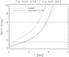 |
Fig. 1. Theoretical curve of Fe XVIII vs. Ca XIV ratio observed by SUMER, using CHIANTI atomic data (dashed-dotted line) and new data (full line). The range of values observed by Teriaca et al. (2012) in an active region core while several microflares were occurring are shown as dashed lines (i.e. within 1.5 and 6). The SUMER temperatures with the new atomic data are higher, but still less than 4 MK. |
Nonetheless, the maximum observed ratio values were around six, indicating relatively low temperatures of 4 MK at most. It could well be that further improvements in the atomic data for Ca XIV might increase the temperatures further, but not by much. As such, the direct spectroscopic information for one AR from SUMER confirms the Del Zanna (2013a) results, meaning that the presence of Fe XVIII emission in AR cores does not guarantee that temperatures of 7 MK are reached.
3. Data selection and analysis
Data from SDO AIA and Hinode XRT were searched to identify suitable active regions. We focused on quiescent ARs that were isolated, so that there was no interfering activity with neighboring ARs, which could cause heating events. ARs that exist from limb to limb, or even better, over a full solar rotation, were preferred as they could potentially be studied to see if their behaviour evolves over their full lifetimes. GOES X-ray fluxes were analysed to avoid flaring ARs. Various tools such as Helioviewer were used. As AIA observes the disc continuously, the main selection criterion was to find XRT multi-filter observations with at least a one-minute cadence, observing continuously for at least a few hours. We selected several ARs and microflares, and present here as a test case one event, as in this case we also had simultaneous Hinode EIS spectra with a high cadence (four minutes), which we could then use to validate the temperature results from XRT.
3.1. Hinode – EIS
We used custom-written software to process the EIS level-0 data (see, e.g. Del Zanna et al. 2011b). We applied the Del Zanna (2013b) radiometric calibration. We then fitted all the available lines with Gaussian profiles, and spatially co-aligned the two EIS channels with the AIA observations.
3.2. Hinode – XRT
We adopted the standard SolarSoft programs to process the data (Kobelski et al. 2014). First, applying xrt_prep with de-spiking and de-spotting (using keyword /despike_despot) and co-aligning with AIA pointing as reference (keyword coalign=1), level 1 data is produced, along with grade maps that indicate bad (saturated, hot spots, etc.) areas or pixels. Then we removed jittering (xrt_ jitter) with reference to time 14:22. XRT images were then co-aligned with respect to AIA, using the AIA 94 Å Fe XVIII images.
We calculated the XRT temperature responses using the effective areas calculated for the specific dates, CHIANTI v.8 (Del Zanna et al. 2015b), and photospheric abundances, although we note that the choice of chemical abundances does not affect the results based on the filter ratios presented here. From the responses we obtained the isothermal temperatures using the filter ratios.
Figure 2 shows one example, indicating that the ratio could in principle be used to measure temperatures between 1 and 10 MK, although the signal towards lower temperatures decreases, so in effect, the filters are useful to measure temperatures above 2 MK.
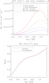 |
Fig. 2. XRT Be-thin and Ti-poly temperature responses and their ratio. |
3.3. SDO – AIA
We used the AIA cutout service, but applied our own cross-correlation to account for solar rotation, using the 1700 Å images. Despite having only about 1 Å width, the AIA 94 Å channel contains several emission lines, as discussed in Del Zanna (2013a). This spectral band was chosen because of the presence of a hot Fe XVIII line at 93.932 Å. The images clearly showed the presence of multi-thermal material (Del Zanna et al. 2011b) and several studies were devoted to understanding this band.
Significant progress was provided by Del Zanna (2012) with the identification of an Fe XIV 93.61 Å line, which is the dominant contribution to the 94 Å band in any AR observation, whenever Fe XVIII is not present. Further progress was due to the improvement of the atomic data for the known Fe X 94.012 Å line with a new scattering calculation (Del Zanna et al. 2012). The atomic calculations of O’Dwyer et al. (2012) indicated instead that Fe VIII and Fe IX contributions to the band are not large.
Del Zanna (2013a) used simultaneous EIS spectra and AIA observations, combined with the known ratios between the soft X-ray and EUV lines, to develop an atomic-based method to estimate the Fe XVIII count rates in the AIA 94 Å channel, IFe XVIII, using the 171 and 211 Å as proxies for the Fe X and Fe XIV contributions. Specifically,
 (1)
(1)
where IAIA 94 Å is the count rate in the AIA 94 Å band, IAIA 211 Å the count rate in the AIA 211 Å band, and IAIA 171 Å the count rate in the AIA 171 Å band. We adopt this method here. One result of their analysis was to indicate that significant Fe XVIII emission is often present in the cores of ARs whenever a high emission measure at 3–4 MK was present.
The contribution function G(T) of the Fe XVIII line is peaked around 7 MK, and has a steep increase from about 2.5 MK. We can simply estimate the increase in the AIA Fe XVIII count rates due solely to an increase in the electron temperature by looking at the increase in the G(T), normalised to the value at 2.5 MK, as shown in Fig. 3. Even a small increase from 2.5 to 3.5 MK would result in an increase of the Fe XVIII count rates by a factor of ten. Clearly, further increases can also be due to increased densities (i.e. emission measures).
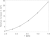 |
Fig. 3. Relative increase in G(T) of AIA Fe XVIII line, normalised to 2.5 MK. |
Finally, we note that other authors (see, e.g. Warren et al. 2012) also developed various methods to remove the cooler contributions to the 94 Å band. However, all these previous approaches were purely empirical.
4. The microflare case study
On 2011 September 3, a series of recurrent microflares were observed by XRT and EIS within the small active region NOAA 11283. The XRT instrument observed the AR with the Be-thin and Ti-poly filters, with about a one-minute cadence. We have selected one of the main microflares.
Figure 4 shows a sequence of AIA negative images in a selection of bands and timings, showing the evolution of the microflare, while Fig. 5 displays the magnetic field configuration as observed by SDO’s Helioseismic and Magnetic Imager (HMI) with overlayed AIA 94 Å contours. The event shows the appearance of two loops that became activated simultaneously. Some strong brightenings appeared at the footpoints of the loops, and indicate the locations of increased densities in the regions where chromospheric evaporation is occurring (for a discussion on signatures of chromospheric evaporation in small flares see Del Zanna et al. 2011a). Some other weak features appear to be connecting the footpoints of the loops and two nearby small jets that become activated at the same time (they are outside the FOV of the images). We selected a region near the top of the lower loop structure to obtain light curves and temperatures from XRT and EIS.
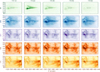 |
Fig. 4. Sequence of AIA negative images in selection of bands and timings. These images show the evolution of the microflare that occurred on 2011 September 3 at 14:20 UT. The box indicates the lower loop-top region chosen for detailed study. |
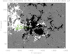 |
Fig. 5. SDO HMI line-of-sight magnetogram of the active region NOAA 11283 at the time the microflare was observed, with the SDO AIA 94 Å contour overlayed in green. |
Figure 6 shows the light curves in a selection of the AIA bands. The peak emission in the AIA 94 Å (Fe XVIII) is around 14:22. Within a few minutes, the loops fade in Fe XVIII and reach peak emission in the 335 Å band after ten minutes, indicating cooling to about 3 MK, as we interpret the peak emission in the 335 Å band as being dominated by Fe XVI, which is formed around 3 MK. Interestingly, very little emission in the cooler AIA bands is present later on. Its spatial distribution is quite different from that of the hotter Fe XVIII and Fe XVI emission. This behaviour is typical of these microflare events and is very different from the behaviour of larger events like GOES B-class (Del Zanna et al. 2011a) or C-class (Petkaki et al. 2012) flares, where the same loop-like structure, which is first seen in higher temperatures, is observed to cool down from about 10–12 MK through 5, 3, 1 MK, and down to chromospheric temperatures.
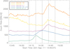 |
Fig. 6. Scaled light curves in selection of AIA bands for lower loop-top region shown in Fig. 4 (boxed area). The vertical dotted lines indicate the timings of the images in Fig. 4. |
Figure 7 shows a snapshot of the microflare during the peak emission, as seen by two of the XRT bands (top two plots). As shown in the bottom plot of Fig. 7, the morphology of the microflare is nearly the same as seen in the XRT and the AIA Fe XVIII emission.
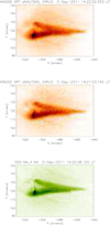 |
Fig. 7. From top to bottom: Hinode XRT Ti-poly and Be-thin images during microflare peak; SDO AIA Fe XVIII emission. The box indicates the top of the lower loop area selected for further analysis. |
The top of Fig. 8 shows the light curves in the XRT bands and AIA Fe XVIII in the loop-top region. As a few of the XRT images were saturated (they are indicated with an asterisk), we could not obtain XRT temperatures for those timings. The time differences in the two filters are within a few seconds, and the intrinsic variations in the count rates have been verified as not affecting the temperature measurements. The XRT temperatures of the loop-top region for the timings that were not saturated are shown in the bottom plot of Fig. 8. The XRT indicates a temperature increase from about 3.5 MK to 4.5 MK. We also obtained XRT temperatures using the standard XRT SolarSoft programs, and obtained similar results. The uncertainties in the temperature reflect the Poisson noise in the XRT counts and take into account the theoretical variation of the ratio, as shown in Fig. 2.
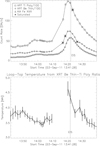 |
Fig. 8. Temporal microflare evolution. Top: averaged count rates of the data inside the box of the two XRT filters (Ti-Poly and Be-Thin, squares and diamonds respectively), both divided by 100, as well as the reconstructed Fe XVIII emission from the AIA filters (triangles). Saturated data points in XRT are marked with an asterisk, and the vertical lines enclose the timing of the EIS observation of the same data interval. Bottom: temporal evolution of the temperature inside the box, obtained from XRT filter ratios. The dashed, vertical line indicates the time of the EIS observation in the same region. |
The increase in the estimated count rates due to Fe XVIII in the AIA 94 Å band in the loop-top region is about a factor of five during the peak. As we measured the temperatures from XRT, it is interesting to see how much of the observed increase is due to the small 1 MK temperature increase (cf. Fig. 3). We therefore took the XRT variation in temperature in the box and calculated the corresponding increase in the AIA Fe XVIII emission, shown in Fig. 9. This is about a factor of four, indicating that the main increase in the AIA 94 Å signal is due to a remarkably small temperature increase. The isothermal approximation used to measure temperatures from XRT also provide the values of the emission measure, which are proportional to the square of the electron density. If we multiply the increase in the Fe XVIII emissivity with the emission measure we obtain the points shown with diamonds in Fig. 9, which are quite close to the observed variation in the AIA Fe XVIII emission.
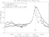 |
Fig. 9. Relative increase in AIA Fe XVIII signal in lower loop-top. These are estimated from the AIA 94 Å signal (triangles), as obtained from the increased emissivity of the line due to the temperature variation obtained from XRT (squares), and as obtained by combining the increase in the emissivity and the emission measure (diamonds). The dashed, vertical lines indicate the timings of the EIS observation during the microflare peak. |
Hinode EIS continuously observed the AR with the study HH_Flare+AR_180×152, using the 2″ slit and 9 s exposure times. The study was a “sparse raster” of 30 slit positions with steps of 6″, covering a FOV of 180 × 152″. Each slit position was observed every about 10 s, and the FOV was covered with a cadence of about four minutes. Only a selection of a few spectral lines was telemetered to the ground.
Figure 10 shows the monochromatic images obtained in the Fe XII and Ca XVII lines before (raster start at 13:41 UT) and during (raster start at 14:19 UT) the microflare. Very few changes in the lines formed below 3 MK (as the Fe XII) were observed. The hotter emission is clearly visible in Ca XVII, and has the same morphology as the XRT and AIA Fe XVIII, as expected. Brightenings associated with chromospheric evaporation are visible in the footpoint regions of the loops. Figure 11 shows a zoomed-in version of the Ca XVII image during the peak of the microflare, indicating the starting times of each slit position and the location of the box in the lower loop-top.
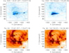 |
Fig. 10. Hinode EIS monochromatic images in Fe XII and Ca XVII before and during main microflare. The box is drawn at the same location of the lower loop-top as in the AIA and XRT images (Figs. 4 and 7). |
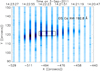 |
Fig. 11. Hinode EIS monochromatic image of Ca XVII line at 192.8 Å of microflare. Due to rastering, data were only recorded at a sparse spatial resolution, with the white stripes indicate data gaps. Each vertical raster is taken 11 s apart. The time-axis is given at the top of the graph, with time running from right to left. The loop-top is marked by the black box, which was selected for further analysis. The spatial coordinates of the data were shifted in order to be aligned with SDO AIA observations. |
Averaged EIS spectra in the box were obtained to increase the S/N ratio for the pre-flare and flare plasma. All the lines were fitted and the calibration was later applied to obtain radiances. A sample of a few spectral windows is given in Appendix A.
To measure the temperature distribution (DEM) of the top of the lower loop, we assumed a spline functional form for the DEM and the method described in Del Zanna (1999). The results for both the pre-flare and flare plasma are shown in Fig. 12. The points are plotted at the effective temperature Teff (the formation T of the line averaged over the DEM), and at the predicted vs. the observed intensity ratio, multiplied by the DEM value at Teff. The respective values of the spectral lines used for the DEM fit shown in Fig. 12 are given in Tables 1 (flaring plasma) and 3 (quiescent plasma), respectively.
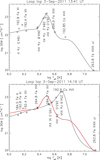 |
Fig. 12. DEM before (top) and during microflare (bottom), obtained from Hinode EIS. The pre-flare DEM is also shown in the bottom plot as a red line. The points are plotted at the effective temperature Teff. The labels indicate the wavelength (Å) and the main ion. |
Observed and predicted radiances for microflare loop-top region, with raster start at 14:19 UT.
The “photospheric” abundances of Asplund et al. (2009) were adopted here as we would expect the flare plasma not to have had the time to develop coronal abundances. However, we note that the DEM is well-constrained by all iron lines, that is, the chemical abundances only constrain the absolute value, not the shape. The 3 MK peak in the pre-flare DEM is typical (Del Zanna 2013a) and well-constrained by lines from Fe XV, FeXVI, and the hotter lines from Ca XVII and Fe XVII, for which upper limits were used.
For the microflare, an upper limit to the 12 MK emission from Fe XXIII 263.8 Å was adopted. This was obtained by measuring the standard deviation of the counts where the line is, to obtain an estimate of the peak emission. This value was then converted to integrated radiances. The result is 3 ergs cm−2 s−1 sr−1, which is the same value as the one obtained by Parenti et al. (2017).
The microflare peak DEM is well-constrained by a significant increase in the Fe XVI and especially the hot Ca XVII and Fe XVII emission. The Fe XVII is weak but measurable, see Fig. A.2. As shown in Fig. A.2, the Ca XVII is significantly blended with Fe XI and O V (see Del Zanna 2008; Del Zanna et al. 2011a for a discussion on blending for this line and the Fe XXIII line). We fit three Gaussian profiles, with a careful selection of the limits in the wavelength and widths of these lines. The monochromatic image in Ca XVII clearly shows that this method works relatively well when the line is strong. Normally, we would estimate the Ca XVII by estimating the Fe XI and O V contributions using other Fe XI and O V lines, but for the present study this was not easily achievable as the other O V line at 248.5 Å was very weak, and the other Fe XI lines in the study were problematic. In fact, the Fe XI 192.63 Å is known to be blended with an un-identified line, while the Fe XI 192.0 Å is blended with at least Fe XXIV and Fe VIII transitions, if not others.
To cross-check that the Ca XVII de-blending was correct, we added the Fe XI and O V de-blended lines to the DEM analysis. The results in Table 1 clearly indicate an excellent agreement for the Fe XI line, which is the main contributor to the blend. Furthermore, the fact that Ca XVII is in excellent agreement with Fe XVII confirms that the de-blending was successful. The O V line at 248 Å is a complex blend and is very weak. This O V line, compared to the O V lines at 192.9 Å is also density-sensitive and so it is difficult to estimate the O V lines. However, it is clear that the O V lines blended with Ca XVII are not very strong, so even if their estimate is wrong by a factor of two, it would not significantly affect the Ca XVII intensity.
The DEM obtained from the Ca XVII and Fe XVII EIS lines indicates a peak emission around 4.5 MK. Considering the pre-flare DEM, the lower loop emission is nearly isothermal. These results are important as they both validate the isothermal assumption used to get temperatures from XRT, and confirm the XRT temperatures. Finally, we note that the difference in the DEM at 3 MK is somewhat misleading, as the Fe abundance at these temperatures is typically increased by a factor of 3.2 over its photospheric value (Del Zanna 2013a).
Having obtained the DEM of the loop-top, we were then able to easily predict the signal in the XRT bands and the estimated AIA Fe XVIII using CHIANTI and the effective areas of the instruments for the specific date as available within SolarSoft. For the forward modelling, we used the same photospheric abundances as the ones that were used for the DEM inversion, and notice that some differences would be present in the predicted XRT count rates if other abundances were used. Table 2 lists these predicted count rates vs. the observed ones for both the XRT Ti-poly and the Be-thin filters, for both photosperic as well as coronal abundances. We calculated the XRT count rates, adding the continuum, and summing all contributions from 2 to 200 Å, using CHIANTI data. The observed count rates in the XRT bands are about 50% higher than predicted. We note that the ratios of the two bands are nearly the same (about two) for all the different columns, observed as well as predicted, regardless of the abundance model. This is reassuring and gives us confidence in the reliability of using this filter ratio to derive a temperature, which in this case is around 4.5 MK (see also Fig. 2).
Observed and predicted (using EIS DEM) Hinode XRT count rates.
The EIS DEM was obtained with a spline node at log T = 6.7, one at 6.8, and the last one at 7.1. The last point was kept fixed. The DEM at log T = 6.8 cannot be increased as this would substantially increase the Ca XVII and Fe XVII line fluxes, which are very sensitive to this temperature. The DEM at log T = 7.1 is unconstrained as we do not have a measurement of the Fe XXIII line. We calculated the XRT count rates obtained by increasing and decreasing the DEM at log T = 7.1 by a factor of 10, and added these results to Table 2. Results show that the two XRT filters are not very sensitive to these changes. This can be explained by the fact that most of the XRT count rates in these two filters come from Fe XVII lines and other lines formed at similar temperatures, as seen in Fig. A.1 and previously discussed in O’Dwyer et al. (2014). We also note that increasing the DEM above 10 MK would increase the emission in the Fe XXIV 192.0 Å line, which would be inconsistent with our EIS observation.
We also tested the effects on the predicted XRT counts related to the chemical abundances. We ran the DEM fitting by adopting the “coronal” abundances of Feldman et al. (1992), where the iron abundance is increased by a factor of about four. We then ran the forward modelling, and obtained the XRT count rates in the last column of Table 2. We can see that assuming coronal abundances worsens the discrepancy between the observed and predicted XRT count rates (from a factor of 1.5 for photospheric to a factor of two for coronal abundances).
In the case of AIA, the EIS DEM predicts 94 DN s−1 pixel−1 for the Fe XVIII emission1. The lower-temperature Fe emission in the AIA band is predicted to be much lower: 2.3 are made in addition to for Fe XIV and 1.3 for Fe X. The observed count rates are about 60, meaning about 50% lower than predicted. This difference could also be due to calibration problems, although we note that the high-temperature tail in the DEM is not well-constrained by the EIS observations, so a difference of 50% is not very large.
4.1. Radiometric calibration issues
We suggest that the observed discrepancies are due to calibration issues with the XRT and the AIA 94 Å band. This issue is complex and cannot be easily resolved. Here, we note a few key points and refer to Appendix B for further information.
The fact that the XRT observed count rates are higher than expected was reported by several authors. Wright et al. (2017) also found a difference of a factor of two when comparing the well-calibrated NuSTAR observations of a microflare with XRT. On the other hand, Fe XVIII flux obtained from the AIA bands was in excellent agreement with NuSTAR. Made in 2015, these observations also adopted the “coronal” abundances of Feldman et al. (1992). With these same coronal abundances, we also find a factor of two discrepancy with XRT. Earlier, Schmelz et al. (2015) suggested a discrepancy of a factor of two in the absolute values of the XRT effective area, for observations from 2011 using coronal abundances (Schmelz et al. 2012). We note that relatively good agreement (∼30%) was found when O’Dwyer et al. (2014) cross-correlated EIS and XRT observations from 2007 December, using coronal abundances, while larger discrepancies (∼50%) were found using photospheric abundances.
Original calibration of XRT in the first 2.5 years of operation (Narukage et al. 2011) for the quiet Sun show that the counts in all the XRT filters have a significant decrease in sensitivity (some by a factor of three within five months). Corrections were implemented. Frequent bake-outs were introduced to increase the sensitivity. A follow-up paper by Narukage et al. (2014) adopted the relative calibration of Ti-poly and Be-thin filters to constrain the calibration of the thick filters, imposing the expectation that the same temperatures should be obtained from the various filter combinations.
To our knowledge, there are no published studies of the long-term, absolute calibration of the XRT channels, so it is quite possible that the degradation of the XRT channels needs to be revisited, especially considering the frequent bake-outs. As mentioned above, the main contributions to the XRT bands in relatively quiescent active regions are from Fe XVII lines. These lines are observable by EIS if there is some microflaring activity, so an estimate of the cross-calibration can be obtained.
The EIS calibration was monitored in-flight until 2012 September (Del Zanna 2013b). The count rates in the cooler lines in the short-wavelength (SW) channel did not indicate any significant degradation, while the line ratios between the long-wavelength and the SW channels did indicate a strong degradation by about a factor of two in the long-wavelength channel within the first few years.
Cross-calibration studies between EIS and the AIA channels on observations in 2010 have indicated very good agreement (Del Zanna et al. 2011b; Del Zanna 2013a). The cross-calibration of the EIS SW and AIA 193 Å channel is straightforward as both channels observed the same spectral range. EIS SW and AIA 193 Å comparisons continue to be made by one of us (GDZ) and by H. Warren (priv. comm.), and have shown good agreement, within 20%.
The cross-calibration with the AIA 94 Å was in agreement with observations from 2010 (Del Zanna 2013a). In Appendix B, we present results from an analysis of an EIS observation taken near the time of our observation (on 2011 October 22). In this case, longer exposures were used and a strong signal in the Fe XVII lines is present. The DEM obtained from the EIS observations predicts AIA 94 Å count rates that are also almost a factor of two higher than observed, as in the microflare presented here.
The calibration of the AIA channels is non-trivial. Some of the channels degraded significantly from 2010. Several bake-outs have been carried out to improve sensitivity, and calibration studies are ongoing. The AIA calibration for the first few years has been monitored against the SDO EVE full-Sun spectra. There are no clear indications that the AIA 94 Å degraded significantly (W. Liu, priv. comm.). Relatively good agreement between AIA and EVE was found in 2010, see for example Del Zanna et al. (2011b). The EVE suffered significant degradation as well, and it was only with the version five of its calibration that a technique similar to that one adopted for the EIS calibration (line ratios) was used, improving the resulting irradiance.
5. Conclusions
We analysed simultaneous EIS, XRT, and AIA observations of a microflare to obtain the following new findings: (a) on the basis of the EIS data, an isothermal approximation is reasonable; (b) the temperature obtained from the XRT filter ratio is in excellent agreement with the peak of the DEM obtained from EIS, and only about 4.5 MK; (c) the small temperature increase (of around 1 MK) of the microflare loop as measured by XRT is nearly sufficient to explain the increase in the AIA Fe XVIII line; and (d) the microflare loop cools rapidly towards the background temperature, and does not appear to cool towards chromospheric temperatures. We have also shown that: (e) as we found in some previous cases, the AIA Fe XVIII line is often formed far from the peak abundance of the ion in equilibrium at 7 MK; a re-analysis of SUMER temperatures obtained from Fe XVIII confirms this. In addition, we have shown that: (f) the timescale of the event is typical, about ten minutes. In terms of absolute values, we found significant inconsistencies (factors of about two) in the cross-calibration of the EIS, XRT, and AIA channels. Further work is needed to try and resolve these discrepancies. However, these inconsistencies do not affect the main results of this paper.
These results encourage us to use the XRT filter ratios to study the temperature evolution of all the microflares we selected in different active regions. This will be discussed in a follow-up paper where we will present further evidence that microflares typically reach temperatures between 4 and 8 MK. On this basis, it is clear that detailed analyses of microflares need spectroscopic observations of emission lines formed in the 3–10 MK range. We point out that there is no current or planned mission to cover this important temperature range, with the exception of the MaGIXS sounding rocket flight, planned for 2019 August.
Finally, it is interesting to note the differences between the microflare presented here and other small flares of GOES B and C-class. We described “textbook” flares of these two classes in Del Zanna et al. (2011a) and Petkaki et al. (2012). In terms of light curves, the larger flares have a steeper increase of the X-ray flux and a more gradual decay, which can last much longer. Presumably all flares have a similar chromospheric evaporation process occurring at the footpoints, as described in detail in Del Zanna et al. (2011a). Flares of B- and C-class always reach 10−12 MK regardless of the size and energy of the event, and their cooling proceeds through all lower temperatures, down to chromospheric temperatures, while the loop plasma drains back to the chromosphere in the same places where it evaporated. The microflare presented here reaches at most 5 MK and shows a sudden cooling to 3 MK. We defer the study of this behaviour with hydrodynamic modelling to a separate paper.
If calibration corrections accounting for differences between AIA and SDO’s EUV Variability Experiment (EVE) (using SolarSoft keyword /eve_norm) are made in addition to using the date-specific, effective area files available within SolarSoft, the predicted count rate for the Fe XVIII emission is even higher (117 DN s−1 pixel−1).
Acknowledgments
We would like to thank the anonymous referee for very helpful comments, which were addressed in the final version of this paper. We acknowledge support by STFC (UK) via a consolidated grant to the solar and atomic astrophysics group at DAMTP, University of Cambridge. Data supplied are courtesy of the SDO/AIA consortium. Hinode is a Japanese mission developed and launched by ISAS/JAXA, with NAOJ as domestic partner and NASA and STFC (UK) as international partners. It is operated by these agencies in co-operation with ESA and NSC (Norway). CHIANTI is a collaborative project involving the University of Cambridge (UK), George Mason University, the University of Michigan, and Goddard Space Flight Centre (USA). We found Helioviewer, the European Hinode science data centre, and the Lockheed Martin Solar and Astrophysics Laboratory (LMSAL) AIA data centre very useful.
References
- Asplund, M., Grevesse, N., Sauval, A. J., & Scott, P. 2009, ARA&A, 47, 481 [NASA ADS] [CrossRef] [Google Scholar]
- Brosius, J. W., Daw, A. N., & Rabin, D. M. 2014, ApJ, 790, 112 [NASA ADS] [CrossRef] [Google Scholar]
- Cargill, P. J. 2014, ApJ, 784, 49 [NASA ADS] [CrossRef] [Google Scholar]
- Del Zanna, G. 1999, PhD Thesis, Univ. of Central Lancashire, UK [Google Scholar]
- Del Zanna, G. 2008, A&A, 481, L69 [NASA ADS] [CrossRef] [EDP Sciences] [Google Scholar]
- Del Zanna, G. 2012, A&A, 546, A97 [NASA ADS] [CrossRef] [EDP Sciences] [Google Scholar]
- Del Zanna, G. 2013a, A&A, 558, A73 [NASA ADS] [CrossRef] [EDP Sciences] [Google Scholar]
- Del Zanna, G. 2013b, A&A, 555, A47 [NASA ADS] [CrossRef] [EDP Sciences] [Google Scholar]
- Del Zanna, G., & Ishikawa, Y. 2009, A&A, 508, 1517 [NASA ADS] [CrossRef] [EDP Sciences] [Google Scholar]
- Del Zanna, G., & Mason, H. E. 2003, A&A, 406, 1089 [NASA ADS] [CrossRef] [EDP Sciences] [Google Scholar]
- Del Zanna, G., & Mason, H. E. 2014, A&A, 565, A14 [NASA ADS] [CrossRef] [EDP Sciences] [Google Scholar]
- Del Zanna, G., & Mason, H. E. 2018, Liv. Rev. Sol. Phys., 15 [Google Scholar]
- Del Zanna, G., Mitra-Kraev, U., Bradshaw, S. J., Mason, H. E., & Asai, A. 2011a, A&A, 526, A1 [NASA ADS] [CrossRef] [EDP Sciences] [Google Scholar]
- Del Zanna, G., O’Dwyer, B., & Mason, H. E. 2011b, A&A, 535, A46 [NASA ADS] [CrossRef] [EDP Sciences] [Google Scholar]
- Del Zanna, G., Storey, P. J., Badnell, N. R., & Mason, H. E. 2012, A&A, 541, A90 [NASA ADS] [CrossRef] [EDP Sciences] [Google Scholar]
- Del Zanna, G., Tripathi, D., Mason, H., Subramanian, S., & O’Dwyer, B. 2015a, A&A, 573, A104 [NASA ADS] [CrossRef] [EDP Sciences] [Google Scholar]
- Del Zanna, G., Dere, K. P., Young, P. R., Landi, E., & Mason, H. E. 2015b, A&A, 582, A56 [NASA ADS] [CrossRef] [EDP Sciences] [Google Scholar]
- Feldman, U., Mandelbaum, P., Seely, J. F., Doschek, G. A., & Gursky, H. 1992, ApJS, 81, 387 [NASA ADS] [CrossRef] [Google Scholar]
- Feldman, U., Doschek, G. A., & Behring, W. E. 1996a, ApJ, 461, 465 [NASA ADS] [CrossRef] [Google Scholar]
- Feldman, U., Doschek, G. A., Behring, W. E., & Phillips, K. J. H. 1996b, ApJ, 460, 1034 [NASA ADS] [CrossRef] [Google Scholar]
- Hannah, I. G., Christe, S., Krucker, S., et al. 2008, ApJ, 677, 704 [NASA ADS] [CrossRef] [Google Scholar]
- Hannah, I. G., Grefenstette, B. W., Smith, D. M., et al. 2016, ApJ, 820, L14 [NASA ADS] [CrossRef] [Google Scholar]
- Ichimoto, K., Hara, H., Takeda, A., et al. 1995, ApJ, 445, 978 [NASA ADS] [CrossRef] [Google Scholar]
- Ishikawa, S.-N., Glesener, L., Christe, S., et al. 2014, PASJ, 66, S15 [NASA ADS] [CrossRef] [Google Scholar]
- Kirichenko, A. S., & Bogachev, S. A. 2017, ApJ, 840, 45 [NASA ADS] [CrossRef] [Google Scholar]
- Klimchuk, J. A. 2006, Sol. Phys., 234, 41 [NASA ADS] [CrossRef] [Google Scholar]
- Ko, Y., Doschek, G. A., Warren, H. P., & Young, P. R. 2009, ApJ, 697, 1956 [NASA ADS] [CrossRef] [Google Scholar]
- Kobelski, A. R., Saar, S. H., Weber, M. A., McKenzie, D. E., & Reeves, K. K. 2014, Sol. Phys., 289, 2781 [NASA ADS] [CrossRef] [Google Scholar]
- Mrozek, T., Gburek, S., Siarkowski, M., et al. 2018, Sol. Phys., 293, 101 [NASA ADS] [CrossRef] [Google Scholar]
- Narukage, N., Sakao, T., Kano, R., et al. 2011, Sol. Phys., 269, 169 [NASA ADS] [CrossRef] [Google Scholar]
- Narukage, N., Sakao, T., Kano, R., et al. 2014, Sol. Phys., 289, 1029 [NASA ADS] [CrossRef] [Google Scholar]
- O’Dwyer, B., Del Zanna, G., Badnell, N. R., Mason, H. E., & Storey, P. J. 2012, A&A, 537, A22 [NASA ADS] [CrossRef] [EDP Sciences] [Google Scholar]
- O’Dwyer, B., Del Zanna, G., & Mason, H. E. 2014, A&A, 561, A20 [NASA ADS] [CrossRef] [EDP Sciences] [Google Scholar]
- Parenti, S., del Zanna, G., Petralia, A., et al. 2017, ApJ, 846, 25 [NASA ADS] [CrossRef] [Google Scholar]
- Parker, E. N. 1988, ApJ, 330, 474 [Google Scholar]
- Peter, H., Bingert, S., Klimchuk, J. A., et al. 2013, A&A, 556, A104 [NASA ADS] [CrossRef] [EDP Sciences] [Google Scholar]
- Petkaki, P., Del Zanna, G., Mason, H. E., & Bradshaw, S. J. 2012, A&A, 547, A25 [NASA ADS] [CrossRef] [EDP Sciences] [Google Scholar]
- Reale, F. 2010, Sol. Phys., 7, A5 [Google Scholar]
- Reva, A., Shestov, S., Zimovets, I., Bogachev, S., & Kuzin, S. 2015, Sol. Phys., 290, 2909 [NASA ADS] [CrossRef] [Google Scholar]
- Rosner, R., Tucker, W. H., & Vaiana, G. S. 1978, ApJ, 220, 643 [NASA ADS] [CrossRef] [Google Scholar]
- Saba, J. L. R., & Strong, K. T. 1991, ApJ, 375, 789 [NASA ADS] [CrossRef] [Google Scholar]
- Schmelz, J. T., Reames, D. V., von Steiger, R., & Basu, S. 2012, ApJ, 755, 33 [NASA ADS] [CrossRef] [Google Scholar]
- Schmelz, J. T., Asgari-Targhi, M., Christian, G. M., Dhaliwal, R. S., & Pathak, S. 2015, ApJ, 806, 232 [NASA ADS] [CrossRef] [Google Scholar]
- Shimizu, T. 1995, PASJ, 47, 251 [NASA ADS] [Google Scholar]
- Sterling, A. C., Hudson, H. S., & Watanabe, T. 1997, ApJ, 479, L149 [NASA ADS] [CrossRef] [Google Scholar]
- Sylwester, B., Sylwester, J., Siarkowski, M., Engell, A. J., & Kuzin, S. V. 2011, Cent. Eur. Astrophys. Bull., 35, 171 [NASA ADS] [Google Scholar]
- Teriaca, L., Warren, H. P., & Curdt, W. 2012, ApJ, 754, L40 [NASA ADS] [CrossRef] [Google Scholar]
- van Ballegooijen, A. A., Asgari-Targhi, M., Cranmer, S. R., & DeLuca, E. E. 2011, ApJ, 736, 3 [NASA ADS] [CrossRef] [Google Scholar]
- Warren, H. P., Brooks, D. H., & Winebarger, A. R. 2011, ApJ, 734, 90 [NASA ADS] [CrossRef] [Google Scholar]
- Warren, H. P., Winebarger, A. R., & Brooks, D. H. 2012, ApJ, 759, 141 [NASA ADS] [CrossRef] [Google Scholar]
- Watanabe, T., Haka, H., Shimizu, T., et al. 1995, Sol. Phys., 157, 169 [NASA ADS] [CrossRef] [Google Scholar]
- Winebarger, A. R., Warren, H. P., Schmelz, J. T., et al. 2012, ApJ, 746, L17 [NASA ADS] [CrossRef] [Google Scholar]
- Wright, P. J., Hannah, I. G., Grefenstette, B. W., et al. 2017, ApJ, 844, 132 [NASA ADS] [CrossRef] [Google Scholar]
Appendix A: Additional information on the microflare event of 2011 September 3
Figure A.1 shows the predicted spectra for the Be-thin (top) and the Ti-Poly (bottom) Hinode XRT filters, respectively, in the microflare loop-top region, using temperature and emission measure obtained from Hinode EIS.
Figure A.2 displays a selection of Hinode EIS lines from the microflare loop-top region: the well-resolved Fe XI at 192.0 Å and Fe XII at 192.4 Å with photon-counts in the hundreds (top-left), the barely resolved Fe XVII at 254.9 Å with a base-to-peak photon-count increase of around 20 (bottom-left), and the wavelength region from 263.2−264.2 Å, where the hot Fe XXIII line would be, which is not detected within the random count fluctuations of around ten counts (bottom-right). The top-right image shows the fit to the Ca XVII line (192.7−193.0 Å), which is blended with Fe XI as well as O V, where the dashed lines indicate the individual ions, and the solid, smooth line indicates the total of the individual contributions added up.
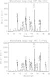 |
Fig. A.1. Hinode XRT predicted count rates in microflare loop-top region for Be-thin and Ti-Poly filters. |
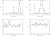 |
Fig. A.2. Selection of EIS windows in microflare loop-top region. The spectra are in data numbers (DN) as a function of wavelength (Å). |
Appendix B: An EIS vs. AIA 94 Å cross-calibration study – 2011 October 22
Considering the discrepancies between the estimated and predicted AIA count rates, we searched the Hinode EIS database to try and find a suitable observation to verify this cross-calibration. We found a full-spectral observation on 2011 October 22, with the 2″ slit and 60 s exposures, which therefore has a lot more signal than the microflare observation presented here. The raster duration was about one hour. The core of an AR was observed during the last 1/2 h, when several small microflare loops appeared across the entire AR core. Several short-lived loops are visible in the AIA 94 Å band, and are also clearly visible in several Fe XVII lines in EIS. No emission in Fe XXIII or Fe XXIV was observed.
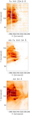 |
Fig. B.1. Top: monochromatic image in Fe XVII of EIS raster on 2011 October 22. A microflare region selected for DEM analysis is shown with a box. Middle: estimated Fe XVIII emission in the AIA 94 Å band, downgraded to the spatial and temporal resolution of the EIS raster. Bottom: AIA 94 Å band image. |
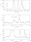 |
Fig. B.2. Sample EIS spectral ranges of microflare region on 2011 October 22. |
Figure B.1 (top) shows a monochromatic image in the strongest Fe XVII line. The bottom plot in the figure shows a reconstructed AIA 94 Å image, obtained by downgrading the AIA spatial and temporal resolution to that of the EIS observation, following a procedure outlined in, for example Del Zanna et al. (2011b). The middle plot shows the same AIA image but where the cooler contributions to the band have been removed, following Del Zanna (2013a). It is clear that an exact agreement between the AIA and EIS images is not present. This is partly due to the difference in the exposure times for each pixel, partly due to the jittering and the point spread function of the EIS instrument which is not simple to reproduce.
However, the main features are clearly visible. We took a large area (the box displayed in the Fig. B.1) as representative of the ensemble of microflare loops, and measured the average count rates in the AIA band. We obtained 23 DN s−1 per AIA pixel, and 16 in the estimated Fe XVIII count rates.
We averaged the EIS spectra in the area, measured the line intensities and performed a DEM analysis. A sample of a few spectral regions is shown in Fig. B.2. The resulting DEM is shown in Fig. B.3, and the observed vs. predicted intensities in Table B.1. We found an excellent agreement between observed and predicted intensities in all the main Fe XVII lines, identified and discussed in Del Zanna & Ishikawa (2009), as well as between the Fe XVII and Ca XVII line intensities. As most of the emission in the area comes from the diffuse AR core emission, we used “coronal abundances”, although the predicted AIA count rates are independent of the choice given that all the main lines contributing to the band are from iron.
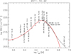 |
Fig. B.3. DEM of microflare region on 2011 October 22. The black line was derived using an upper limit for the Fe XXIII count rates, while the red line had this limit set to 0. |
Observed and predicted radiances for microflares region on 2011 October 22 (same layout as Table 1).
For the Fe XXIII, we adopted a similar upper limit as for the microflare from 2011 September 3 analysed in the main article. It should be noted that the peak ion abundances of Ca XVII and Fe XVII are log T[K] = 6.75, meaning quite close to the peak ion abundance of Fe XVIII (T[K] = 6.85). As the Fe XVIII ion abundance has a significant tail towards lower temperatures, it turns out that a significant portion of the Fe XVIII emission comes from the same temperature plasma that emits Fe XVII and Ca XVII. As these ions are also sensitive to emission around log T[K] = 6.85, the slope of the DEM is well-constrained at such a temperature. In other words, the estimated Fe XVIII emission is relatively well-constrained by the emission measures from Fe XVII and Ca XVII. The Fe XXIII provides a further upper limit of around 10 MK. With the DEM shown in Fig. B.3, we estimate a count rate of 29 DN s−1 for the AIA Fe XVIII. The Fe XIV and Fe X contribute about 4 DN s−1 and the rest of the lines and continuum another 4. Decreasing the DEM in the poorly constrained higher temperatures, as shown in Fig. B.3 by the red line, only decreases the predicted Fe XVIII signal to 26 DN s−1. This observation from 2011 October 2, which has a much higher signal and more spectral lines than the one from 2011 September 3, confirms the discrepancy between the estimated observed AIA Fe XVIII count rates and the predicted ones from the EIS DEM modelling, with values here of 16 DN s−1 pix−1 (observed) vs. 29 DN s−1 pix−1 (predicted).
All Tables
Observed and predicted radiances for microflare loop-top region, with raster start at 14:19 UT.
Observed and predicted radiances for microflares region on 2011 October 22 (same layout as Table 1).
All Figures
|
Fig. 1. Theoretical curve of Fe XVIII vs. Ca XIV ratio observed by SUMER, using CHIANTI atomic data (dashed-dotted line) and new data (full line). The range of values observed by Teriaca et al. (2012) in an active region core while several microflares were occurring are shown as dashed lines (i.e. within 1.5 and 6). The SUMER temperatures with the new atomic data are higher, but still less than 4 MK. |
| In the text | |
|
Fig. 2. XRT Be-thin and Ti-poly temperature responses and their ratio. |
| In the text | |
|
Fig. 3. Relative increase in G(T) of AIA Fe XVIII line, normalised to 2.5 MK. |
| In the text | |
|
Fig. 4. Sequence of AIA negative images in selection of bands and timings. These images show the evolution of the microflare that occurred on 2011 September 3 at 14:20 UT. The box indicates the lower loop-top region chosen for detailed study. |
| In the text | |
|
Fig. 5. SDO HMI line-of-sight magnetogram of the active region NOAA 11283 at the time the microflare was observed, with the SDO AIA 94 Å contour overlayed in green. |
| In the text | |
|
Fig. 6. Scaled light curves in selection of AIA bands for lower loop-top region shown in Fig. 4 (boxed area). The vertical dotted lines indicate the timings of the images in Fig. 4. |
| In the text | |
|
Fig. 7. From top to bottom: Hinode XRT Ti-poly and Be-thin images during microflare peak; SDO AIA Fe XVIII emission. The box indicates the top of the lower loop area selected for further analysis. |
| In the text | |
|
Fig. 8. Temporal microflare evolution. Top: averaged count rates of the data inside the box of the two XRT filters (Ti-Poly and Be-Thin, squares and diamonds respectively), both divided by 100, as well as the reconstructed Fe XVIII emission from the AIA filters (triangles). Saturated data points in XRT are marked with an asterisk, and the vertical lines enclose the timing of the EIS observation of the same data interval. Bottom: temporal evolution of the temperature inside the box, obtained from XRT filter ratios. The dashed, vertical line indicates the time of the EIS observation in the same region. |
| In the text | |
|
Fig. 9. Relative increase in AIA Fe XVIII signal in lower loop-top. These are estimated from the AIA 94 Å signal (triangles), as obtained from the increased emissivity of the line due to the temperature variation obtained from XRT (squares), and as obtained by combining the increase in the emissivity and the emission measure (diamonds). The dashed, vertical lines indicate the timings of the EIS observation during the microflare peak. |
| In the text | |
|
Fig. 10. Hinode EIS monochromatic images in Fe XII and Ca XVII before and during main microflare. The box is drawn at the same location of the lower loop-top as in the AIA and XRT images (Figs. 4 and 7). |
| In the text | |
|
Fig. 11. Hinode EIS monochromatic image of Ca XVII line at 192.8 Å of microflare. Due to rastering, data were only recorded at a sparse spatial resolution, with the white stripes indicate data gaps. Each vertical raster is taken 11 s apart. The time-axis is given at the top of the graph, with time running from right to left. The loop-top is marked by the black box, which was selected for further analysis. The spatial coordinates of the data were shifted in order to be aligned with SDO AIA observations. |
| In the text | |
|
Fig. 12. DEM before (top) and during microflare (bottom), obtained from Hinode EIS. The pre-flare DEM is also shown in the bottom plot as a red line. The points are plotted at the effective temperature Teff. The labels indicate the wavelength (Å) and the main ion. |
| In the text | |
|
Fig. A.1. Hinode XRT predicted count rates in microflare loop-top region for Be-thin and Ti-Poly filters. |
| In the text | |
|
Fig. A.2. Selection of EIS windows in microflare loop-top region. The spectra are in data numbers (DN) as a function of wavelength (Å). |
| In the text | |
|
Fig. B.1. Top: monochromatic image in Fe XVII of EIS raster on 2011 October 22. A microflare region selected for DEM analysis is shown with a box. Middle: estimated Fe XVIII emission in the AIA 94 Å band, downgraded to the spatial and temporal resolution of the EIS raster. Bottom: AIA 94 Å band image. |
| In the text | |
|
Fig. B.2. Sample EIS spectral ranges of microflare region on 2011 October 22. |
| In the text | |
|
Fig. B.3. DEM of microflare region on 2011 October 22. The black line was derived using an upper limit for the Fe XXIII count rates, while the red line had this limit set to 0. |
| In the text | |
Current usage metrics show cumulative count of Article Views (full-text article views including HTML views, PDF and ePub downloads, according to the available data) and Abstracts Views on Vision4Press platform.
Data correspond to usage on the plateform after 2015. The current usage metrics is available 48-96 hours after online publication and is updated daily on week days.
Initial download of the metrics may take a while.