| Issue |
A&A
Volume 628, August 2019
|
|
|---|---|---|
| Article Number | A51 | |
| Number of page(s) | 16 | |
| Section | Extragalactic astronomy | |
| DOI | https://doi.org/10.1051/0004-6361/201834574 | |
| Published online | 06 August 2019 | |
Reddening map and recent star formation in the Magellanic Clouds based on OGLE IV Cepheids⋆
Aryabhatta Research Institute of Observational Sciences (ARIES), Manora Peak, Nainital 263002, India
e-mail: This email address is being protected from spambots. You need JavaScript enabled to view it.
Received:
5
November
2018
Accepted:
11
June
2019
Abstract
Context. The reddening maps of the Large Magellanic Cloud (LMC) and Small Magellanic Cloud (SMC) are constructed using the Cepheid period–luminosity (P–L) relations.
Aims. We examine reddening distribution across the LMC and SMC through large data sets on classical Cepheids provided by the OGLE Phase IV survey. We also investigate the age and spatio-temporal distributions of Cepheids to understand the recent star formation history in the LMC and SMC.
Methods. The V and I band photometric data of 2476 fundamental mode (FU) and 1775 first overtone mode (FO) Cepheids in the LMC, and 2753 FU and 1793 FO Cepheids in the SMC were analysed for their P–L relations. We converted the period of FO Cepheids to the corresponding period of FU Cepheids before combining the two modes of Cepheids. Both galaxies were divided into small segments and combined FU and FO P–L diagrams were drawn in two bands for each segment. The reddening analysis was performed on 133 segments covering a total area of about 154.6 deg2 in the LMC and 136 segments covering a total area of about 31.3 deg2 in the SMC. By comparison with well-calibrated P–L relations of these two galaxies, we determined reddening E(V − I) in each segment and equivalent reddening E(B − V) assuming the normal extinction law. The period–age relations were used to derive the age of the Cepheids.
Results. Reddening maps were constructed using reddening values in different segments across the LMC and SMC. We find clumpy structures in the reddening distributions of the LMC and SMC. From the reddening map of the LMC, highest reddening of E(V − I) = 0.466 mag is traced in the region centred at α ∼ 85.°13, δ ∼ −69.°34 which is in close vicinity of the star forming HII region 30 Doradus. In the SMC, maximum reddening of E(V − I) = 0.189 mag is detected in the region centred at α ∼ 12.°10, δ ∼ −73.°07. The mean reddening values in the LMC and SMC are estimated as E(V − I)LMC = 0.113 ± 0.060 mag, E(B − V)LMC = 0.091 ± 0.050 mag, E(V − I)SMC = 0.049 ± 0.070 mag, and E(B − V)SMC = 0.038 ± 0.053 mag.
Conclusions. The LMC reddening map displays heterogeneous distribution having small reddening in the central region and higher reddening towards the eastern side of the LMC bar. The SMC has relatively small reddening in its peripheral regions but larger reddening towards the south-west region. In these galaxies, we see evidence of a common enhanced Cepheid population at around 200 Myr ago which appears to have occurred due to a close encounter between the two clouds.
Key words: methods: data analysis / surveys / stars: variables: Cepheids / Magellanic Clouds / galaxies: star formation
Full Tables 1 and 3 are only available at the CDS via anonymous ftp to cdsarc.u-strasbg.fr (130.79.128.5) or via http://cdsarc.u-strasbg.fr/viz-bin/qcat?J/A+A/628/A51
© ESO 2019
1. Introduction
The Large Magellanic Cloud (LMC) and Small Magellanic Cloud (SMC), together known as Magellanic Clouds (MCs) are among one of the most studied galaxies in the Universe due to their close proximity to the Milky Way; they are located at the distance of ≈50 kpc and 60 kpc, respectively (Westerlund 1991; Hilditch et al. 2005; Keller & Wood 2006; de Grijs & Bono 2015). The MCs offer an excellent opportunity to explore many astronomical mechanisms such as star formation, structure formation, and distribution of interstellar medium through a wide range of tracers and they have significantly advanced our understanding of galaxy evolution and dynamical interaction (e.g. Harris & Zaritsky 2004; Skowron et al. 2014; Ripepi et al. 2014; Piatti et al. 2015; Nidever et al. 2017). The MCs provide the ideal laboratory to probe the spatially resolved star formation history (SFH) and dust distributions since these galaxies are not just close enough to be resolved into stars but are also moderately affected by the interstellar extinction and foreground Milky Way stars (Rubele et al. 2018). In recent times, the distribution of different stellar populations in the MCs has been studied by various authors (e.g., Alcock et al. 1999; Pietrzynski & Udalski 1999, 2000; Nikolaev et al. 2004; Borissova et al. 2004, 2006; Harris & Zaritsky 2009; Glatt et al. 2010; Cioni et al. 2011; Subramanian & Subramaniam 2013; Joshi & Joshi 2014; Jacyszyn-Dobrzeniecka et al. 2016; Nayak et al. 2016; Joshi et al. 2016; Rubele et al. 2018; Choi et al. 2018). For example, Borissova et al. (2004, 2006) suggested the existence of a homogeneous, old, and metal-poor stellar halo in the LMC based on the velocity dispersion of RR Lyrae stars. On the basis of spatial and age distributions of Cepheids reported in the Optical Gravitational Lensing Experiment (OGLE) Phase-III survey, Joshi & Joshi (2014) and Joshi et al. (2016) concluded that major star formation was triggered in these two dwarf galaxies at ≈200 ± 50 Myr ago. Choi et al. (2018) revealed a significant warp in the southwest region of the outer disk of the LMC towards the SMC and an off-centred tilted LMC bar which they believe is consistent with a direct collision between the two clouds in agreement with the earlier studies (e.g. Besla et al. 2012, Carrera et al. 2017; Zivick et al. 2018, 2019). On the basis of VMC data in the near-infrared (NIR) filters, Rubele et al. (2018) provided maps for the mass distribution of stars of different ages, and a total mass of all the stars ever formed in the SMC. These kinds of studies are possible due to the availability of an enormous amount of data generated by large sky surveys in these directions, such as the Massive Compact Halo Objects Survey (Alcock et al. 1995), the Optical Gravitational Lensing Experiment (Udalski et al. 1997), the Magellanic Clouds Photometric Survey (Zaritsky et al. 1997), Two Micron All Sky Survey (Skrutskie et al. 2006), the VISTA survey of Magellanic Clouds system (Cioni et al. 2011), the Survey of the MAgellanic Stellar History (Nidever et al. 2017), and so on.
It has long been observed that reddening (a measurement of the selective total dust extinction) information is one of the important parameters used to estimate the structure of the disk of the MCs as well as to derive SFH in these two dwarf galaxies. For example, Subramanian & Subramaniam (2013) suggested that the extra-planer features which are found both in front of and behind the disk could be in the plane of the disk itself if an under-estimate or over-estimate of the extinction values in the direction of the LMC was found. Rubele et al. (2018) derived the extinction AV varying between ∼0.1 mag and 0.9 mag across the SMC and found that the high-extinction values follow the distribution of the youngest stellar populations. By simultaneously solving SFH, mean distance, reddening, and so on, they were able to obtain a more reliable picture of how the mean distances, extinction values, star formation rate (SFR), and metallicities vary across the SMC. Choi et al. (2018) presented an E(g − i) reddening map across the LMC disk through the colour of red clump (RC) stars and suggested that the majority of the reddening toward the non-central regions results from the Milky Way foreground, which acts as a dust screen on stars behind it. They were able to explore the detailed 3D structure of the LMC and detect a new stellar warp by using their accurate and precise 2D reddening map in the LMC disk.
In our analysis, we use classical Cepheids or Population I Cepheids (we hereafter simply refer to both as Cepheids) to map the reddening and probe the recent SFH within the MCs. Cepheids are relatively young massive stars in the core He-burning phase and occupy the space in a well-defined instability strip in the H–R diagram. These are regarded as an excellent tracer for understanding recent star formation in the host galaxy and represent one of the most important findings of the cosmic distance ladder. They play a pivotal role in structure studies of nearby external galaxies, such as MCs, M 31, and M 33, among others, as they are found in many in these galaxies. These pulsating variables, because of their large intrinsic brightness and periodic luminosity variation over time, can be easily detected in the outskirts of the Galactic disk and in nearby galaxies.
Cepheids pulsate in two modes: one called the FU mode in which all parts of the system move sinusoidally with the same frequency and a fixed phase relation, and another called the FO Cepheids which pulsate with short periods and small amplitudes. The distinction between FU and FO Cepheids can easily be made using their positions in the P–L diagram. Cepheids pulsating in the FO mode are about 1 mag brighter and are lower in amplitude than the FU mode for the same pulsation period (e.g. Udalski et al. 1999; Bono et al. 2005). One can also distinguish the two modes through the Fourier parameters R21 and ϕ21 determined from the shape of their light curves. During the past few decades, many studies have been directed towards understanding the structure and reddening distribution in the MCs employing the Cepheids (e.g. Udalski et al. 1999; Nikolaev et al. 2004; Subramanian & Subramaniam 2015; Joshi & Joshi 2014; Joshi et al. 2016; Inno et al. 2016; Scowcroft et al. 2016).
In the present study, we primarily aim to understand the reddening variation across the MCs through multi-band P–L relations of the Cepheids by taking advantage of the largest and most homogeneous sample of FU and FO Cepheids spread all across the MCs in the recently released catalogue of the OGLE-IV survey. Here, we construct a large number of narrow sub-regions in these two galaxies and select a significant number of Cepheids in each sub-region to draw respective P–L diagrams. Furthermore, we convert the period of FO Cepheids to the corresponding period of FU Cepheids in order to make a single P–L diagram with an increased sample size. Using the multi-band P–L diagrams in each sub-region, we then estimate the corresponding reddening values. In this way, we obtain the reddening in all such sub-regions that are used to construct the reddening map which is of vital importance to studying the dust distribution within different regions of these two galaxies. We also estimate the age of Cepheids in order to probe the recent SFH in the two clouds.
This paper is structured as follows. In Sect. 2, we provide details of the data used in the present study. The spatial distribution of Cepheids in the MCs is described in Sect. 3. The reddening determinations and construction of reddening maps are presented in Sect. 4. Our analysis of the Cepheid age determination and recent SFH in the MCs is given in Sect. 5. A discussion, and conclusions of this study are given in Sect. 6.
2. Data
There have been many surveys for Cepheids in the MCs, however OGLE1 has revolutionized the field by producing thousands of Cepheid light curves in the Milky Way, the LMC, and the SMC. OGLE achieved a high signal-to-noise ratio and was used to determine parameters like periods, magnitudes, and amplitudes with great accuracy. OGLE begun its survey in 1992 in its first phase, followed by three more phases appending additional sky coverage. The fourth phase of OGLE survey was carried out using a 32-chip mosaic CCD camera on the 1.3 m Warsaw University Telescope at Las Campanas Observatory, Chile, between 2010 March and 2015 July, which has increased observing capabilities by almost an order of magnitude compared to the OGLE-III phase and covered over 3000 deg2 in the sky (Soszyński et al. 2016). Exhaustive details of the reduction procedures, photometric calibrations, and astrometric transformations are available in Udalski et al. (2015).
Recently the OGLE-IV survey released high-quality photometric data in the V and I bands from their observations of the Magellanic System (Soszyński et al. 2015, 2017). This work utilizes the publicly available photometric catalog of variable stars consisting of 4704 Cepheids in the LMC and 4945 Cepheids in the SMC. The LMC Cepheids sample consists of 2476 FU, 1775 FO, 26 second-overtone (SO), 95 double-mode FU/FO, 322 double-mode FO/SO, 1 double mode FO/Third overtone (TO), 1 double mode SO/TO, and 8 triple-mode Cepheids (Soszyński et al. 2015). Similarly, the SMC sample consists of 2753 FU, 1793 FO, 91 SO, 68 FU/FO, 239 FO/SO, and one triple-mode Cepheid (Soszyński et al. 2017). The sample is reported to be over 99% complete making it the most complete and least contaminated sample of Cepheids in the Magellanic system (Jacyszyn-Dobrzeniecka et al. 2016). For the present study, we only used the archival V and I band data containing the mean magnitude and period of FU and FO Cepheids for both the dwarf galaxies. In total, we used simultaneous V and I band data of 4251 Cepheids in the LMC and 4546 Cepheids in the SMC. The photometric uncertainty on OGLE-IV mean magnitudes is found to be σI, V = 0.007 mag for brighter and longer-period Cepheids (0.7 ≤ log P ≤ 1.5) and σI, V = 0.02 mag for fainter and shorter-period Cepheids (log P < 0.7) (Inno et al. 2016).
3. Spatial distribution
During the last several years, a large number of studies based on different stellar populations have been carried out to understand the structure of the MCs (e.g. Glatt et al. 2010; Wagner-Kaiser & Sarajedini 2013; Subramanian & Subramaniam 2013; Joshi & Joshi 2014; Joshi et al. 2016; Muraveva 2018). In the present study, we have a total of 4251 Cepheids in the LMC and 4546 Cepheids in the SMC. This is the largest sample of Cephieds so far, providing a chance to examine their spatial distributions within the clouds in order to understand the geometry of the disk of these galaxies. To carry out this analysis, we first converted the (RA, Dec) coordinates to (X, Y) coordinates using the relations given by Van De Kamp (1967). We then divided the LMC into 45 × 45 segments with a dimension of 0.4 × 0.4 kpc square for each segment, achieving a mean spatial resolution of ≈1.2 deg2. We divided the SMC into 90 × 90 segments with a smaller dimension of 0.2 × 0.2 kpc square, obtaining a mean spatial resolution of ≈ 0.22 deg2 because the SMC contains a higher density of Cepheids in its relatively small area. We kept the same spatial cell size for all subsequent analyses of our study. The cell size was chosen in such a way that we can get enough Cepheids in each cell for a statistically meaningful determination of mean reddening and recent SFH measurements. Our selection resulted in 389 segments covering a total area of about 456.7 deg2 in the LMC and 562 segments covering a total area of about 131.3 deg2 in the SMC. We counted the total number of Cepheids in each segment in the LMC and SMC and constructed a spatial map of Cepheid distribution.
In Fig. 1, we show the 2D spatial distribution of Cepheids in each of the 389 segments in the LMC. The colour code in the map represents the number of Cepheids in each segment. The observed spatial map in the LMC shows some interesting structures. The centre of the Cepheids density region in the LMC is found to be at X = −1.2, Y = −0.8 which corresponds to the coordinates  and
and  . It is apparent that the stellar overdensities do not match with the optical centre of the LMC but are shifted far away in southeast direction. The spatial distribution of Cepheids along the disk is very distinctive and a bar structure is conspicuous where most of the Cepheids are located. It is also seen that the density structure of the bar region is not smooth. Many Cepheids are distributed in the clumpy structure along the bar which is elongated in the east–west direction where the eastern side of the bar shows a higher density of Cepheids as compared to its western side. On the basis of RC stars in the LMC, the presence of warp in the bar was also noticed by Subramaniam (2003) indicating a dynamically disturbed structure for the LMC. The spatial density of Cepheids in the LMC is found to be very poor in its northern arm.
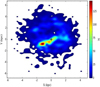 |
Fig. 1. Two-dimensional spatial map in the LMC as a function of the number of Cepheids measured in different segments. North is up and east is to the left. The location of the optical centre of the LMC is shown by a plus symbol. |
In Fig. 2, we present a similar 2D spatial map for the SMC constructed from 562 segments of our chosen size. As one can see in the map, the disk of the SMC seems to be quite irregular and asymmetric. It is evident that the southwestern region of the SMC is the most populated and the centroid of the Cepheids density distribution is located at  ,
,  . While the dense region is much farther away in the LMC from its optical centre, the centroid of the most populated region of Cepheids lies very close to the optical centre in the SMC.
4. Reddening
4.1. Methodology of reddening determination
The dust and gas is heterogeneously distributed within the MCs and a differential extinction is found to exist in these two galaxies. Therefore, a constant extinction cannot be applied in deriving P–L relations across the LMC and SMC. However, one can study the extinction variation in these galaxies by determining reddening in small sub-regions. Since thousands of Cepheids are available in the MCs, we can divide both the galaxies into small segments containing tens of Cepheids in each zone. For each segment, a P–L diagram is plotted in the form of
 (1)
(1)
where mλ, aλ, P, and ZPλ denote apparent magnitude, P–L slope, period of Cepheid, and zero point, respectively, for a given bandpass. Once slope aλ is known through calibrated P–L relations, one can obtain the ZPλ.
As OGLE data is given in V and I bands and many calibrated P–L relations for Cepheids have been derived in these bands in the past studies for the MCs (e.g. Udalski et al. 1999; Laney & Stobie 1994; Freedman et al. 2001; Sandage et al. 2004, 2009; Ngeow et al. 2009, 2015), we used the most recent ones given by Ngeow et al. (2009) for the LMC FU Cepheids as follows:
 (2)
(2)
 (3)
(3)
For the SMC FU Cepheids, we used the P–L relation given by Ngeow et al. (2015) as follows:
 (4)
(4)
 (5)
(5)
where MV and MI denote absolute magnitudes in V and I bands, respectively. We note here that no significant metallicity gradient has been seen across the LMC and SMC (e.g. Grocholski et al. 2006; Cioni 2009; Parisi et al. 2009; Feast et al. 2010; Deb & Singh 2014; Joshi et al. 2016) hence any variation in the MCs P–L relations due to metallicity variation is not considered in the present study. Even if we accept any variation in the metallicity at all, as reported in some previous studies (e.g. Tammann et al. 2003; Carrera et al. 2008; Kapakos & Hatzidimitriou 2012; Dobbie et al. 2014), the difference in reddening is found to be ∼0.001 mag which is insignificant in comparison to the scatter in the P–L diagrams itself. Moreover, many studies have reported a non-linearity in the P–L relations in these galaxies (EROS Collaboration 1999; Udalski et al. 1999; Sharpee et al. 2002; Kanbur & Ngeow 2004; Sandage et al. 2009; Soszyński et al. 2010; Tammann et al. 2011; Subramanian & Subramaniam 2015; Bhardwaj et al. 2016). A wide range of break points has been reported at different places in the P–L diagrams (1.0, 2.5, 2.9, 3.55, and 10 day) which also varies in different bands and different overtones. However, we did not consider any breaks in the P–L diagrams because uncertainties from photometry and low number statistics in the present data were larger than the uncertainties from breaks. With these assumptions, we determine the reddening in a large number of segments across the two galaxies.
It has been observed through the P–L diagram of FU and FO Cepheids however that for the same pulsation period FU Cepheids have greater magnitude as compared to FO Cepheids and they follow two different P–L relations. Therefore, to combine the FU and FO Cepheids together in a single P–L diagram, the period of FO Cepheids needs to be converted into the corresponding period of FU Cepheids, which requires a well-defined relation connecting the two periods. As the vast majority of Cepheids pulsate only in a single mode, there are only a limited number of Cepheids which pulsate in two modes simultaneously (Lemasle et al. 2018). Using the high-resolution spectroscopic observations of 17 such double-mode Galactic Cepheids, Sziládi et al. (2007) derived a relation for transformation of FO and FU periods as follows:
![Mathematical equation: $$ \begin{aligned} \frac{P_{1}}{P_{0}}&= -0.0143~\log P_{0}-0.0265~\left[\frac{\mathrm{Fe}}{\mathrm{H}}\right]+0.7101 \\&\quad {\pm }0.0025 \;\; {\pm }0.0044 \;\; {\pm }0.0014, \nonumber \end{aligned} $$](/articles/aa/full_html/2019/08/aa34574-18/aa34574-18-eq12.gif) (6)
(6)
where P1 and P0 denote the period of FO Cepheids and the corresponding period of FU Cepheids, respectively, and ![Mathematical equation: $ \left[\frac{\mathrm{Fe}}{\mathrm{H}}\right] $](/articles/aa/full_html/2019/08/aa34574-18/aa34574-18-eq13.gif) denotes the metallicity. We converted periods of FO Cepheids to those of the corresponding periods of FU Cepheids to draw P–L diagrams of the combined sample of FU and FO Cepheids. Here, we considered a mean present-day metallicity of −0.34 ± 0.03 dex for the LMC based on Cepheids (Keller & Wood 2006) and −0.70 ± 0.07 dex for the SMC based on supergiants (Hill et al. 1997; Venn 1999).
denotes the metallicity. We converted periods of FO Cepheids to those of the corresponding periods of FU Cepheids to draw P–L diagrams of the combined sample of FU and FO Cepheids. Here, we considered a mean present-day metallicity of −0.34 ± 0.03 dex for the LMC based on Cepheids (Keller & Wood 2006) and −0.70 ± 0.07 dex for the SMC based on supergiants (Hill et al. 1997; Venn 1999).
In Figs. 3 and 4, we illustrate V and I band P–L diagrams in the LMC and SMC, respectively. In each diagram, we show FU and FO Cepheids independently in the left panel and combined FU and FO Cepheids in the right panel after the period conversion. The FU and FO Cepheids can clearly be seen to follow two different P–L relations and after converting FO periods to corresponding FU periods using Eq. (6), they fall on a single P–L relation in their respective filters in both the LMC and SMC, as can be seen in the right plots of Figs. 3 and 4. This approach allows us to combine two different modes of Cepheids in a single P–L relation which in turn gives us a larger sample of Cepheids for the study. We subsequently drew multi-band period versus magnitude diagrams in each segment and fitted the calibrated P–L relation to determine the corresponding intercept. The difference in intercepts between calibrated and observed P–L relations yields the ZP value for a given passband:
 (7)
(7)
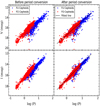 |
Fig. 3. Left panels: P–L diagrams in the LMC for the FU and FO Cepheids. Right panels: combined FU and FO Cepheids after converting the period of FO Cepheids to corresponding periods of FU Cepheids. Upper panels: V filter. Lower panels: I filter. Blue and red points are for FU and FO Cepheids, respectively. |
where ZPcalibrated in the V and I bands are taken as, respectively, 17.115 mag and 16.629 mag for the LMC and 17.606 and 17.127 for the SMC as given in the Eqs. (2)–(5). The ZPobserved varies for each segment mainly according to their relative dust extinction, whereas the P–L slope is almost fixed in a galaxy. Once we know the ZP values in two different passbands, we derive the reddening in the selected region by subtracting them as follows:
 (8)
(8)
where ZPV and ZPI are the zero points in the V and I bands, respectively.
Assuming that the MCs Cepheids follow the same reddening law as that of Galactic Cepheids, we can determine reddening E(B − V) using the following reddening ratio (Wagner-Kaiser & Sarajedini 2017):
 (9)
(9)
In this way, one can estimate reddening E(V − I) and E(B − V) in each segment of the LMC and SMC. The uncertainties in E(V − I) and E(B − V)) values are calculated by combining the error in the ZP values and those in the P–L slopes. It is important to note here that one does not require any prior information on the distance of the host galaxy of Cepheids to map the reddening when their multi-band photometry is available. Since we have V and I band photometry for thousands of Cepheids in the MCs, it ideally suited us to study the reddening in detail in these two nearby clouds which is crucial to understanding the dust distribution and probing the recent SFH in the MCs.
4.2. Reddening in the MCs
Although one can measure the reddening corresponding to each Cepheid, the mean magnitude of each individual Cepheid determined through the photometric light curves may contain some uncertainty, which is propagates in the reddening estimation. Therefore, to carry out our analysis, we made small segments in the LMC and SMC as defined in Sect. 3. To draw P–L relations, we need to select those segments which have a larger number of Cepheids lying in the same direction in order to determine more precise values for the mean reddening with less uncertainty in any given direction. Therefore, only those segments containing a minimum of ten Cepheids (3 × Poissonian error) in at least one passband were considered.
4.2.1. The LMC
We selected a total of 133 segments with an average angular resolution of ≈1.2 deg2 covering a total area of about 154.6 deg2 in the LMC. The maximum number of Cepheids among selected segments is found to be 144 in the LMC. Keeping the slopes fixed in the V and I band P–L diagrams as given in Eqs. (2) and (3), we estimated ZP values for each segment using a least-square fit to the observed period-versus-magnitude diagrams. It should be noted here that uncertainties in the measurements of apparent V and I magnitudes are not provided in the OGLE-IV catalogue and therefore individual photometric errors are not considered in the fit.
In Fig. 5, we show one such randomly selected P–L diagram, in both the V and I band. Here we apply a 3σ cut to reduce contamination in an iterative manner unless all the Cepheids fall within 3σ lines of the given P–L slope where σ is the rms derived from fitting the P–L relation to the observed data points. In Fig. 5, the best-fit slope is drawn as a continuous line while the final 3-σ deviation is shown by dashed lines on both sides of the best fit. It should be noted here that some intrinsic dispersion in the P–L diagram is obvious due to the finite width of the Cepheid instability strip as well as contamination due to blending and crowding effects (Sandage & Tammann 1968; Joshi et al. 2003, 2010). On average, the dispersion in the LMC Cepheid P–L diagrams is found to be ≲0.06 mag in both V and I band. We note here that an uncertainty in the LMC metallicity of 0.03 dex (Keller & Wood 2006) used in Eq. (6) gives only an added 0.001 mag error in the ZP values determined through combined (FU+FO) P–L relations which is much smaller than the typical error on the ZP estimations. Using the zero-point intercepts in V and I band, we determined the reddening E(V − I) and E(B − V) values as described in Eqs. (8) and (9) for all the 133 segments in the LMC. Table 1 lists the central coordinates of all the selected segments in the LMC, and the corresponding reddening values E(V − I) and E(B − V). The complete table is available at the CDS. The value of reddening E(V − I) in different segments of the LMC varies from 0.041 mag to 0.466 mag with a mean value of 0.134 ± 0.006 mag. The histogram shown in Fig. 6 illustrates the distribution of reddening E(V − I) in the LMC.
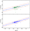 |
Fig. 5. P–L relations for a sub-region in the LMC in the V band (upper panel) and I band (lower panel). Here, the continuous lines represent the best linear fit with a fixed slope of −2.769 for the V band and −2.961 for the I band, respectively. The dashed lines represent the 3σ cut lines and Cepheids outside 3σ lines are shown by open circles which are not considered in the best fit. |
Reddening in 133 different segments of the LMC.
The probability distribution function of interstellar column density measurements is known to be close to log-normal in the solar neighbourhood (e.g. Lombardi et al. 2010). Therefore, we drew a log-normal profile in the reddening distribution of the LMC. The best profile illustrated by the dashed line in Fig. 6 can be seen to match the distribution with exquisite accuracy. The uncertainty in the reddening E(V − I) was determined from the σ-value in the best-fit profile and error in the ZP values in V and I band. Firstly, we calculated error in each value of ZP using the uncertainties in the slope and zero points of the P–L relation in both the filters. The combined error in the estimation of E(V − I) was then determined through the error propagation.
![Mathematical equation: $$ \begin{aligned} \sigma (E(V-I)) = \sqrt{[\sigma (\mathrm{ZP}_V)]^2 + [\sigma (\mathrm{ZP}_I)]^2 + [\sigma (\mathrm{fit})]^2}. \end{aligned} $$](/articles/aa/full_html/2019/08/aa34574-18/aa34574-18-eq17.gif) (10)
(10)
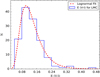 |
Fig. 6. Histogram of reddening values in 133 segments of the LMC shown by continuous line. The dashed line represents the best fit with a log-normal distribution. |
We determined the error in each value of E(V − I) which is given in the last column of Table 1. A mean error in the E(V − I) values was taken corresponding to the peak in the distribution of σ(E(V − I)) values obtained in all 136 segments. The mean value of reddening using the log-normal profile fit is found to be E(V − I) = 0.113 ± 0.060 mag. The corresponding mean value of E(B − V) is estimated as 0.091 ± 0.050 mag.
The reddening in the LMC has been estimated by several authors in the past and we summarize some of the recent reddening measures in E(B − V) or E(V − I) using different stellar populations in Table 2. Among some of the most recent estimates of reddening in the LMC, the RC stars used by Haschke et al. (2011) indicated a mean reddening of the LMC of E(V − I) = 0.09 ± 0.07 mag while with RR Lyrae stars a median value of E(V − I) = 0.11 ± 0.06 mag was obtained. Inno et al. (2016) provided reddening estimates derived through Cepheids at seven different positions across the LMC and found that E(B − V) varies in the range 0.08 ± 0.03 mag to 0.12 ± 0.02 mag. Furthermore, a broader range of E(B − V) from 0.10 ± 0.02 mag to 0.16 ± 0.02 mag was given by Pietrzyński et al. (2013) using detached eclipsing binaries found in the OGLE data. Choi et al. (2018) constructed a 2D reddening map of the LMC disk with help of RC stars observed in the Survey of the MAgellanic Stellar History (SMASH) and reported an average E(g − i) = 0.15 ± 0.05 mag. Using the conversion equations from Abbott et al. (2018), this reddening corresponds to E(B − V) = 0.093 ± 0.031 mag. From the Table 2, it is found that the mean LMC reddening varies from E(B − V) ≈ 0.031 mag to E(B − V) ≈ 0.353 mag. The average LMC reddening E(V − I) = 0.113 ± 0.060 mag and E(B − V) = 0.091 ± 0.050 mag estimated in the present study is in good agreement with the recently reported average reddening measurements using stellar populations of different ages in the LMC.
Summary of recent reddening measurements using different stellar populations in the LMC.
4.2.2. The SMC
Employing the same approach, we selected 136 segments in the SMC with an average angular resolution of ≈0.22 deg2 covering a total area of about 31.3 deg2. The maximum number of Cepheids among selected segments is found to be 80 in the SMC. We plotted period versus magnitude diagrams for each segment and drew a least-square linear fit keeping the slopes fixed in the V and I band P–L diagrams as given in Eqs. (4) and (5). We also applied a 3σ iterative rejection criteria here to remove the outliers. In Fig. 7, we show one such randomly selected P–L diagram along with the best-fit line, both in V and I band. We also illustrate 3-σ cut lines on both sides of the best fit to represent the acceptable deviations in the P–L relation. Employing the same approach as that used for the LMC, we determined the reddening values of E(V − I) and E(B − V) in each of the 136 segments in the SMC. Here, we found that 9 segments (6.6%) have unphysical negative values of reddening and we assigned them zero reddening within the given uncertainties. It should also be noted here that the uncertainty in the SMC metallicity of 0.07 dex (Hill et al. 1997; Venn 1999) used in Eq. (6) only results in an additional 0.001 mag error in the ZP values which is negligible in comparison of the combined uncertainty in the reddening estimates.
Table 3 provides reddening values E(V − I) and corresponding E(B − V) for each segment in the SMC. The complete table is available at the CDS. The value of reddening E(V − I) in different segments within the SMC varies from 0.0 to 0.189 mag with a mean value of 0.064 ± 0.008 mag. The histogram shown in Fig. 8 illustrates the distribution of reddening E(V − I) across the SMC. After fitting a log-normal profile in the histogram, mean value of reddening is estimated to be E(V − I) = 0.049 ± 0.070 mag. The equivalent reddening E(B − V) in the SMC is estimated to be 0.038 ± 0.053 mag.
The reddening in the SMC has been studied by several authors in the past through reddening measures in E(B − V) or E(V − I) using different tracers and we provide the mean reddening values obtained in some of the recent studies (Table 4). Among the most recent analyses, Haschke et al. (2011) obtained a mean value of E(V − I) = 0.07 ± 0.06 mag through 1529 RRab stars of the OGLE-III survey and E(V − I) = 0.04 ± 0.06 mag using RC stars. A mean reddening of E(B − V) = 0.071 ± 0.004 mag was reported by Scowcroft et al. (2016) using a sample of 92 SMC Cepheids with periods greater than 6 days. Muraveva (2018) estimated a reddening of E(V − I) = 0.06 ± 0.06 mag using the VISTA and OGLE-IV survey data of 2997 fundamental mode RR Lyrae stars. Using infrared colour-magnitude diagrams on the deep VISTA survey data, Rubele et al. (2018) inferred a large extinction in the central region of the SMC, but found a relatively lower extinction in the external regions of the SMC. If we compare our present estimates of E(V − I) = 0.049 ± 0.070 mag and E(B − V) = 0.038 ± 0.053 mag with the recent reddening values given in Table 4, we find that our analysis is in broad agreement with the previous studies, except that of Subramanian & Subramaniam (2015), which yielded a higher reddening value of E(B − V) = 0.096 ± 0.080 mag from their study of SMC Cepheids. Tables 2 and 4 also show that the mean reddening values obtained in the MCs through different stellar populations do not show any significant variation among different studies.
Summary of recent reddening measurements using different stellar populations in the SMC.
4.3. Reddening maps in the LMC and SMC
Reddening maps are often generated to remove the effects of reddening from the optical and UV images of different regions of galaxies. They also have wide implications in understanding SFRs and recent SFH in galaxies. In the following sections, we individually focus our attention on the reddening distributions across the LMC and SMC.
4.3.1. The LMC
Through examination of individual estimates of reddening values determined through P–L relations, we found that the reddening varies from one region of the cloud to another. While in some regions of the LMC, reddening is negligible, in other regions it is found to be significantly high. The reddening values estimated for the 133 selected segments were used to construct a reddening map on a rectangular grid using the central (X, Y) of all segments. Figure 9 presents the reddening map derived through the P–L diagrams of the Cepheids, showing the mean reddening along the line of sight toward each segment. Here, a smoothed reddening distribution was adopted to construct the map. The optical centre of the LMC ( and
and  ; de Vaucouleurs & Freeman 1972) is shown. The quality of a reddening map is regulated by the size of the segments as well as the number of Cepheids available in these regions. The sparse spatial distributions of the LMC Cepheids in the outer regions, as shown in Fig. 1, lead to poor resolution in the reddening map in the outer regions of the LMC as seen in Fig. 9.
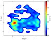 |
Fig. 9. Reddening maps emanating from the P–L diagrams of the Cepheids in the LMC. North is up and east is to the left. The optical centre of the LMC is shown by a plus symbol. The colour bar represents the interpolated reddening E(V − I). |
The reddening map of the LMC exhibits a non-uniform distribution of dust across the LMC. With respect to the optical centre in the LMC, a lopsidedness in the reddening distribution towards the eastern regions can be seen. While the central region of the LMC contains low values of reddening, that is, E(V − I) = 0.113 ± 0.045 mag, the most promising region in the LMC reddening map is seen towards the northeast region of the outer disk of the LMC centred at X = −1.6 kpc, Y = 0.0 kpc from the centre, which corresponds to  with E(V − I) = 0.466 mag. Interestingly, the adjacent region centred around α ∼ 84°, δ ∼ −70° contains the highest concentration of Cepheids in our sample. This region is most likely associated with the star forming HII region 30 Doradus (Tarantula Nebula or NGC 2070) centred at
  (Høg et al. 2000). This is the most active star forming region in the bar of the LMC (Kim et al. 1999; Tatton et al. 2013). The same region was identified as having the highest reddening by Nikolaev et al. (2004) and Inno et al. (2016) as well as having the highest concentration of young cluster populations by Glatt et al. (2010). This region lies in the direction of the compact massive cluster RMC 136a that contains a large concentration of young star clusters (Glatt et al. 2010; Evans 2011). Ochsendorf et al. (2017) found that 30 Dor is located in the region where the LMC bar joins the H I arms and such locations are prone to enhanced star formation activity due to high concentrations of gas and to the shocks induced by the internal dynamical processes (Bitsakis et al. 2018). In the bar region across the LMC disk, reddening is relatively low and a mean value of E(V − I) = 0.153 mag was estimated. On the other side of the LMC bar, a few extinguished regions are found with moderate reddening. The reddening map is generally in good agreement with the maps of HI column density (Luks & Rohlfs 1992) and MACHO Cepheids (Nikolaev et al. 2004). The geometry of the LMC disk was studied by Nikolaev et al. (2004) using the MACHO and 2MASS Cepheids data and estimated the mean reddening E(B − V) by three different methods. All three of the estimated reddening values were consistent with each other and the variance-weighted average reddening was found to be E(B − V) = 0.14 ± 0.02 mag.
It is found that the reddening maps of the LMC have been constructed in numerous studies in the past using different kinds of stellar populations. In order to compare our reddening map with some of the recent studies in the LMC, we took advantage of four such reddening maps in the LMC constructed in the optical bands for which archival data are available (cf., Subramaniam 2005; Haschke et al. 2011; Nayak et al. 2016; Inno et al. 2016). We performed a cell-by-cell comparison of our reddening map with these latter published maps after cross-examinations of central (α, δ) values of each segment with the reddening values given in the same region in these maps. The histograms of the comparisons between our reddening map and the published maps are illustrated in Fig. 10. We discuss these comparisons in some detail below.
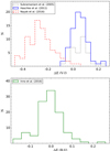 |
Fig. 10. Upper panel: distribution of the ΔE(V − I), i.e. the results of past studies subtracted from our results in the LMC as mentioned in the top-left corner. Lower panel: difference ΔE(B − V) between our reddening estimates and those of Inno et al. (2016). |
-
The reddening E(V − I) values in the LMC are estimated by Subramaniam (2005) for 1123 locations and the E(V − I) found in the LMC varies between 0.1 and 0.3 mag. This latter study shows the total average LMC bar reddening is E(V − I) = 0.08 ± 0.04 mag and eastern regions have higher reddening as compared to western regions. We carried out cell-by-cell comparison of E(V − I) obtained in our study with that of the Subramaniam (2005) as shown in Fig. 10a with the dotted line which shows that reddening values estimated by Subramaniam (2005) are marginally underestimated in comparison with our studies.
-
Haschke et al. (2011) estimated reddening E(V − I) using RR Lyrae stars and RC stars from OGLE-III data. They reported low reddening in the central bar regions of the LMC and higher reddening towards 30 Doradus region, which was also noticed in the present study. In Fig. 10a, we show a difference of our estimated reddening values with those of Haschke et al. (2011) with a continuous line and both studies are found to be in close agreement.
-
Nayak et al. (2016) studied 1072 star clusters in the LMC using OGLE-III data and a semi-automated quantitative method was used to estimate the age and reddening of these clusters. Their E(V − I) values range from 0.05 to 0.50 mag with maximum reddening lying between 0.1 and 0.3 mag. The distribution of the cell-by-cell comparison shown in Fig. 10a with a dashed line peaks at ∼ − 0.28 mag, which means that the reddening given by Nayak et al. (2016) is much higher in comparison to other studies carried out in the LMC in recent times.
-
Inno et al. (2016) investigated the LMC disk using Cepheids in OGLE-IV data. Figure 10(b), illustrates a comparison between E(B − V) values derived in the present study and those of Inno et al. (2016). The histogram shows that the two studies are in excellent agreement within the quoted uncertainties. This result also endorses our approach of combining two modes of Cepheids in a single P–L relation in order to estimate reddening measurements.
In general, we find our reddening map to be in excellent agreement with recent reddening studies in the optical region, except that of Nayak et al. (2016). The histograms shown in Fig. 10 also provide an opportunity to examine the difference in the reddening estimates traced through different stellar populations. It can be seen from Fig. 10 that while Subramaniam (2005) and Haschke et al. (2011) yield smaller reddening values from the older stellar populations RC and RR Lyrae stars, the map constructed by Nayak et al. (2016) gives higher reddening values using the young star clusters in comparison with Cepheid variables which are relatively intermediate age stellar populations. It is also found that Inno et al. (2016), who also used Cepheids in their study as in the present analysis, obtain similar reddening estimates to ours. In general, younger populations like open clusters are likely to be more embedded in the dusty clouds and therefore provide larger reddening than the older populations like RC stars and RR Lyraes.
4.3.2. The SMC
The reddening values determined for 136 selected segments within the SMC were used to construct a reddening map, which is illustrated in Fig. 11. The optical centre of the SMC ( and
and  ; de Vaucouleurs & Freeman (1972)) is shown in the same figure. The reddening map exhibits a non-uniform and highly clumpy structure across the SMC. The peripheral regions of the SMC show smaller reddening in comparison to the central regions. The reddening is larger in the southwest parts of the SMC. The largest reddening in the SMC is found to be E(V − I) = 0.189 in the region centred at X = 0.3, Y = −0.3 which corresponds to
  . On average, the reddening values in the SMC are found to be E(V − I) = 0.049 ± 0.070 mag and E(B − V) = 0.038 ± 0.053 mag, which are substantially smaller in comparison to the mean reddening values in the LMC. If we compare the reddening maps in the LMC and SMC shown in Figs. 9 and 11 with the spatial distributions of Cepheids given in Figs. 1 and 2, it is interesting to note that the reddening structures are found to be approximately correlated with those of the spatial distributions of Cepheids in both galaxies, particularly in the SMC where higher reddening has been observed in close vicinity of the densely populated regions of Cepheids.
Reddening maps of the SMC have been presented by many authors in the past using different kinds of stellar populations (Schlegel et al. 1998; Zaritsky et al. 2002; Dobashi et al. 2009; Haschke et al. 2011; Subramanian & Subramaniam 2015; Rubele et al. 2018; Nayak et al. 2018). Below, we discuss a comparative study of our reddening map with some of the recent studies carried out in the SMC.
-
Haschke et al. (2011) studied the SMC reddening E(V − I) using RR Layrae and RC stars from the OGLE-III data. The continuous line in Fig. 12 shows the difference between reddening E(V − I) estimated by us and Haschke et al. (2011) using RC stars. The distribution peaks at 0.02 mag suggesting that reddening values determined by Haschke et al. (2011) are slightly smaller in comparison to those of our study.
-
Nayak et al. (2018) studied 179 open clusters within the SMC using the same techniques as they used for the LMC open clusters. We show a comparison of the present reddening estimates with those of Nayak et al. (2018) in Fig. 12 as a dashed line. The distribution peaks at −0.08 mag, which means that Nayak et al. (2018) reddening values are larger in comparison to our estimates. A similar comparison carried out earlier in Sect. 4.3.1 for the LMC also shows that the reddening estimates of these latter authors are higher in comparison to those presented here.
-
Rubele et al. (2018) constructed a reddening map using 14 deep tile images taken in the YJKs filters during the VMC survey and found a range of extinction (AV) between ∼0.1 mag (external regions) and 0.9 mag (inner regions). Comparing our reddening map with those of Rubele et al. (2018) in the 32 common regions, we find that our E(B − V) values are smaller in comparison to theirs. In the lower panel of Fig. 12, we present a histogram of the differences between our reddening estimates and those of Rubele et al. (2018) which shows a range of variations peaking around −0.08 mag. We however note that the study carried out by Rubele et al. (2018) is based on near-IR data whereas our reddening estimates are based on optical data.
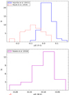 |
Fig. 12. Upper panel: distributions of ΔE(V − I), i.e. past reddening estimates subtracted from our estimate in the SMC as mentioned in the top-left corner. Lower panel: difference of E(B − V) from Rubele et al. (2018) subtracted from our reddening estimate. |
It is evident from the histograms in Fig. 12 that Haschke et al. (2011), who used an older stellar population, found lower reddening values, while Nayak et al. (2018), who used a younger stellar population, retrieved higher reddening values in comparison to our reddening estimates in the SMC, a result similar to our previous comparison for the LMC. It is therefore quite clear from these comparative studies that the low reddening values follow the distribution of the older stellar populations and younger populations lead to higher reddening in the MCs.
4.4. Effect on the reddening maps due to different P–L relations
In the present study, we used the most recent P–L relations given by Ngeow et al. (2009, 2015) to determine reddening estimates in the regions of the LMC and SMC, respectively. Many other studies have reported P–L relations, such as Laney & Stobie (1994), Udalski et al. (1999), Freedman et al. (2001), Sandage et al. (2004, 2009), and Ngeow et al. (2009, 2015). To investigate whether or not reddening distributions across the LMC and SMC determined in the present study are effected by the choice of P–L relations used for their determination, we cross-examined the present reddening maps with those determined using the Udalski et al. (1999)P–L relations as well as those obtained using an independent set of P–L relations given by Sandage et al. (2004) for the LMC and Sandage et al. (2009) for the SMC. We used the same methodology as discussed previously in Sect. 4.1 to find reddening values in the MCs and constructed the reddening maps for both the LMC and SMC.
The histogram in the lower panel of Fig. 13 illustrates the difference between our estimates and those determined through previous P–L relations given by Udalski et al. (1999) and Sandage et al. (2004) by continuous and dashed lines, respectively. The reddening estimates obtained in the present study for the LMC using the P–L relations of Ngeow et al. (2009) are in between those obtained using the P–L relations of Udalski et al. (1999) and Sandage et al. (2004). While we obtain slightly lower values of E(V − I) compared to Udalski et al. (1999), we acquired slightly larger E(V − I) values in comparison to Sandage et al. (2004). However, the difference between our estimates and those given in two studies is less than 0.02 mag which is relatively small in comparison to the uncertainties in the reddening estimations themselves. For a quantitative verification of our reddening values, we also present the significance of the differences between different reddening maps in the upper panel of Fig. 13, which illustrates the difference in reddening divided by the reddening uncertainty in each segment. Here, we compare our values with those obtained through the Udalski et al. (1999) and Sandage et al. (2004)P–L relations. These maps suggest excellent quantitative agreement between the reddening maps obtained through different P–L relations in the LMC except for a few isolated segments as shown by blue squares in Fig. 13.
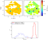 |
Fig. 13. Lower panel: histogram of the difference Δ E(V − I) between the present study and those of Udalski et al. (1999) shown by a continuous line, and Sandage et al. (2004) shown by a dashed line. Upper panel: heat map representing the difference in reddening divided by reddening uncertainty in each segment, left panel – between the present reddening estimates and those of Udalski et al. (1999); right panel – between the present reddening estimates and those of Sandage et al. (2004). The difference is obtained by subtracting the results of other studies from our estimates. |
A similar comparison between the reddening values obtained in the present study using Ngeow et al. (2015)P–L relations and those obtained using the P–L relations of Udalski et al. (1999) and Sandage et al. (2009) is illustrated in Fig. 14 for the SMC. It is conspicuous from the differential plots that the present estimates in the SMC are slightly smaller than those obtained through both Udalski et al. (1999) and Sandage et al. (2009)P–L relations. However, differences lie between 0.02 mag and 0.03 mag which can be considered as non-significant considering the uncertainties involved in the estimation of reddening. In general, we conclude that the choice of Cepheids P–L relations does noticeably effect estimations of reddening in the two clouds.
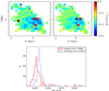 |
Fig. 14. Same as Fig. 13 but for the SMC. Here, comparisons are made between our maps and those obtained by Udalski et al. (1999) and Sandage et al. (2009) using P–L relations. |
5. Recent SFH in the Magellanic Clouds
Recent studies show that major star formation events took place in the MCs at several epochs ranging from a few gigayears to a few million years ago (e.g. Harris & Zaritsky 2004; Rezaeikh et al. 2014; Rubele et al. 2018) though with varying SFRs from field to field (Cignoni et al. 2013; Rubele et al. 2012, 2015)). Therefore, a comprehensive study of Cepheids provides a unique opportunity to probe the recent SFH in the MCs as these are relatively young population and most of them have ages of less than a few hundred million years. Furthermore, the age and spatial-temporal distributions of Cepheids along with MCs structural parameters may provide important information about the formation history of the Magellanic system.
5.1. Age distribution
The P–L and mass–luminosity relations of Cepheids imply that longer-period Cepheids have higher luminosities and are more massive, meaning a relatively shorter life span for these pulsating stars. Therefore, the period and age of Cepheids have an obvious connection. As Cepheids typically have ages in the range of roughly 30–600 Myr, a study of age distribution of Cepheids can be used to reconstruct the recent SFH within the MCs in the last few tens to the last few hundreds of millions of years. Since the pulsation period of Cepheids is the only quantity that can be precisely determined from the observations of the pulsating stars, their ages can be determined with a good accuracy using the period–age (PA) relations.
To determine the ages of Cepheids from their periods, Magnier et al. (1997), Efremov & Elmegreen (1998), and Efremov (2003) proposed many semi-empirical relations and Bono et al. (2005) provided theoretical PA and and period–age–colour (PAC) relations. Recently, Joshi & Joshi (2014) used mean periods of 74 LMC Cepheids found in 25 different open clusters and corresponding cluster ages taken from Pandey et al. (2010) to draw an improved PA relation in the LMC. The empirical PA relation derived by Joshi & Joshi (2014) for the Cepheids in the LMC is given as
 (11)
(11)
where age denoted by t is in years and P is the period given in days. The reliability of the above PA relation has been examined in Joshi & Joshi (2014) by comparing this relation with the Bono et al. (2005) theoretical PA relation determined on the basis of evolutionary and pulsation models covering a broad range of stellar masses and chemical compositions. We found reasonable agreement between the two relations given for the LMC.
The Cepheids PA relation nevertheless varies with metallicity for the galaxies and as we have not derived any such PA relation for the SMC, we considered here a theoretical PA relation given by the Bono et al. (2005) for the SMC. Since we have already converted the periods of the FO Cepheids to corresponding periods of FU Cepheids, we only used the PA relation of FU Cepheids for the known metallicity of the SMC (z = 0.004):
 (12)
(12)
We used the above PA relation to determine the age of each Cepheid in the LMC and SMC. As the error in the periods of the Cepheids is reported to be less than 0.001%, we have not taken it into account in the subsequent age conversion, but the typical average error in age is estimated to be ∼40 Myr due to uncertainty in the PA relations given by Bono et al. (2005) and Joshi & Joshi (2014). Although the resulting ages are in the range of log(t/yr) = 6.96–8.96 with a mean log(t/yr) of 8.21 for the LMC, three quarters of the Cepheid population in the LMC is distributed between log(t/yr) = 8.0 and 8.4. Similarly, although ages for the SMC Cepheids range from log(t/yr) = 6.66 to 8.86 with a mean age of 8.27, about three quarters of them are confined between log(t/yr) = 8.1 and 8.5. One can see that the SMC Cepheids are on average slightly older in comparison to the LMC Cepheids.
We determined the distribution of Cepheids in a bin width of 0.05 dex (on a logarithmic scale) in the LMC and SMC, shown in Figs. 15 and 16, respectively. We see a pronounced peak in the age distribution of Cepheids in the LMC that can be represented by a Gaussian-like profile. In Fig. 15, we show the best-fit Gaussian distribution in the histogram that gives a peak at log(t/yr) = 8.21 ± 0.11. However, a slightly broad profile is evident in the age distribution of Cepheids in the SMC which may be represented by a bi-modal Gaussian profile as has been drawn by Jacyszyn-Dobrzeniecka et al. (2016). Though we do not observe a clear bimodality in the age distribution of SMC Cepheids, a double-Gaussian profile still gives a better fit than a single Gaussian, and therefore we prefer the former. A best-fit double-Gaussian profile in the age histogram, which is shown by a dashed line in Fig. 16, gives a prominent primary peak at log(t/yr) = 8.36 ± 0.08 and a small secondary peak at log(t/yr) = 8.17 ± 0.08. The peak for the younger Cepheids is not strong enough to draw any firm conclusions, although it coincides with the primary peak in the LMC. We note here that the final error in age represents the combined uncertainty in the PA relation, and corresponds to the mean age estimation in the Gaussian fit. The maxima in age distributions of Cepheids indicate a rapid enhancement of Cepheid formation at around  Myr for the LMC and
  Myr for the SMC. The rapid enhancement of Cepheids around 200 Myr ago (within 1-σ uncertainty) in the LMC and SMC points to a major star formation episode at that time, most likely due to a close encounter between the two clouds or their interactions with the Galaxy stem from their multiple pericentric passages as they orbit the Milky Way.
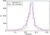 |
Fig. 15. Age distribution of Cepheids in the LMC. The best-fit Gaussian profile is shown by a dashed red line. |
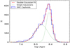 |
Fig. 16. Same as Fig. 15 but for the SMC. The best-fit double-Gaussian profile is shown by a dashed red line and the individual Gaussian is shown as a dotted green line. |
The oscillation between rise and fall in the SFR depends on whether these two clouds are approaching or receding (Glatt et al. 2010; Joshi et al. 2016). This repeated interaction between LMC and gas-rich SMC leads to episodic star formation in these two dwarf galaxies which are locked in tidal interaction. It is believed that the Magellanic Bridge and the Magellanic Stream might have formed due to such interactions in the past between the two segments of the MCs (Besla et al. 2010; Muraveva 2018). As a consequence of these frequent encounters, the tidal stripping of stars and gas or other material from the gaseous disk takes place in the Magellanic system. In fact gas in the Magellanic Bridge is thought to have been largely stripped from the SMC as a consequence of its close interactions with the LMC about 200 Myr ago (Dobbie et al. 2014; Mackey et al. 2017).
Considering several previous studies on the interactions of the clouds (e.g. Besla et al. 2012; Zivick et al. 2018, 2019) there is ample evidence of a direct collision between two clouds with an impact parameter of a few kiloparsecs (Oey et al. 2018; Zivick et al. 2018). These studies along with many previous studies confirm epochs of recent star formation in the MCs albeit at slightly different ages. Using open star clusters in the SMC, Pietrzynski & Udalski (2000) and Glatt et al. (2010) found a peak at 160 Myr through their age distribution. A similar conclusion was also drawn by Subramanian & Subramaniam (2015) using OGLE-III data based on Bono et al. (2005) PAC relation and Jacyszyn-Dobrzeniecka et al. (2016) using OGLE-IV data based on the Bono et al. (2005) PA relation. In a recent investigation by Ripepi et al. (2017) using data from the VISTA near-infrared YJKs survey of the Magellanic system (VMC), the authors also predicted a close encounter or a direct collision between the two cloud components some 200 Myr ago and confirm the presence of a Counter-Bridge.
On the theoretical side, several studies have inferred cloud–cloud interactions in the MCs. In some of the recent models proposed by Bekki & Chiba (2005), Kallivayalil et al. (2006), Diaz & Bekki (2012), Besla et al. (2012), and Zivick et al. (2018), it was suggested that the last cloud–cloud collision within the Magellanic system occurred about 100–300 Myr ago causing enhanced star formation activity in these two dwarf galaxies that might have resulted in the formation of the Magellanic Stream. In fact mutual interactions between the clouds and subsequent tidal stripping of material from the SMC are believed to be the most likely reason for the formation of the Magellanic Bridge (Besla et al. 2012; Diaz & Bekki 2012; Muraveva 2018). This would also mean that the Magellanic Stream and Magellanic Bridge stellar populations should contain stars from both the LMC and the SMC. On the other hand, it was also suggested by Glatt et al. (2010) and references therein; that not only the frequent tidal interaction between the two clouds but also stellar winds and supernova explosions may induce episodic star formation in these two dwarf galaxies.
5.2. Spatio-temporal distribution
The spatial distribution of Cepheids as a function of age is shown in Figs. 17 and 18 for the LMC and SMC, respectively. The figures show that the Cepheids are distributed relatively homogeneously throughout the LMC while preferential distribution of Cepheids is seen in the SMC. From examination of the age map of the LMC, a complex and patchy age distribution is evident, where both young and old Cepheid populations are distributed in small structures across the cloud. We also see a gradual change in the ages of Cepheids from central to peripheral regions where inner regions have lower ages and outer regions have pockets of higher ages as was noted from the last star formation event (LSFE) map presented by Indu & Subramaniam (2011) through the determination of the main-sequence (MS) turn-off point in the colour–magnitude diagram. A similar structure was also observed by Meschin et al. (2014) who suggested a stellar population gradient in the LMC disk where younger stellar populations are more centrally concentrated. These latter authors also proposed an outside-in quenching of star formation in the outer LMC disk (RGC = 3.5 − 6.2 kpc) which might be associated with the variation of the size of the HI disk as a result of gas depletion due to star formation or ram-pressure stripping, or of the compression of the gas disk as ram pressure from the Milky Way halo acted on the LMC interstellar medium.
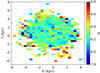 |
Fig. 17. Spatial distributions of the Cepheids in the 389 segments of the LMC as a function of their mean log(t/yr). North is up and east is to the left. The location of the optical centre of the LMC is shown by a plus symbol. |
For the SMC, an age map of the Cepheids shows a systematic distribution where younger Cepheids lie towards inner region and older Cepheids are mainly confined towards peripheral regions. This suggest an inwards quenching of star formation in the SMC. Ripepi et al. (2017) also found that young and old Cepheids have different geometric distributions in the SMC. They observed that closer Cepheids are preferentially distributed in the eastern regions of the SMC which are off-centred in the direction of the LMC owing to a tidal interaction between the two clouds (Muraveva 2018).
If we compare the frequency distribution maps of the Cepheids shown in Figs. 17 and 18 with similar maps made for the star clusters identified in Glatt et al. (2010) (also see Fig. 9 of Joshi & Joshi 2014 for the LMC and Fig. 5 of Joshi et al. 2016 for the SMC), we notice that the clumps of Cepheids do not coincide with the clumps of the star clusters in either of the MCs and a mutual avoidance of clumps of the Cepheids and star clusters is present within the MCs.
6. Discussion and conclusions
The nearby LMC and SMC are the two galaxies for which the highest number of Cepheids is detected, and with excellent data quality. The main motive of this paper was to exploit the available V and I band data of close to nine thousand Cepheids in the MCs. The independent reddening values determined through the multi-wavelength P–L relations of Cepheids are important to construct reddening maps necessary to understand the dust distributions within different regions of the host galaxy. In the present study V and I band photometric data of Cepheids provided by the OGLE-IV photometric survey were analysed to understand the reddening distributions across the LMC and SMC and subsequently to draw reddening maps in these two nearby galaxies. We used 2476 FU and 1775 FO Cepheids in the LMC and 2753 FU and 1793 FO Cepheids in the SMC in the present analysis. In the present study there is one major addition in comparison to other similar studies in that instead of studying individual P–L relations for FU and FO Cepheids, we combined these two modes of pulsating stars after converting periods of FO Cepheids to the corresponding periods of FU Cepheids. This has increased our sample size of Cepheids used to draw P–L diagrams and has allowed us to analyse small size segments within the galaxies leading to an increased resolution of the reddening maps. To reduce statistical error in the reddening estimation, we selected only those segments which contain a minimum of ten Cepheids. We drew a best-fit P–L relation in both V and I band data in all the segments of the LMC as well as those of the SMC. Using the well-calibrated P–L relations for the LMC and SMC, we estimated the reddening E(V − I) in each segment of both the galaxies. We found that the reddening E(V − I) varies from 0.041 mag to 0.466 mag in the LMC and 0.00–0.189 mag in the SMC. The mean value of reddening obtained through a best-fit log-normal profile was found to be E(V − I) = 0.113 ± 0.060 mag and E(B − V) = 0.091 ± 0.050 mag for the LMC. The mean value of reddening obtained through a similar approach in the SMC was estimated to be E(V − I) = 0.049 ± 0.070 mag and E(B − V) = 0.038 ± 0.053 mag.
Using the reddening distributions of 133 segments in the LMC and 136 segments in the SMC, we constructed reddening maps with a cell size of 0.4 × 0.4 square kpc in the LMC and 0.2 × 0.2 square kpc in the SMC. This provides an average angular resolution of about 1.2 deg2 covering an area of 150 deg2 in the LMC, and an angular resolution of about 0.22 deg2 covering an area of 30 deg2 in the SMC. The reddening map of the LMC shows a heterogeneous distribution with lower reddening in the bar region and higher reddening towards northeast region. We did not find any significant reddening in the central region of the LMC. The highest reddening in the LMC, that is E(V − I) = 0.466 mag, was traced in the northeast region located at  and seems to be associated with the most active star forming HII region, 30 Doradus, situated at α ∼ 84°, δ ∼ −70°, which also contains the highest concentration of Cepheids in our sample. In the case of the SMC, the reddening map exhibits a non-uniform and highly clumpy structure across the cloud. In general, lower reddening was found around central regions of the SMC and higher reddening was seen in the southwest region away from the optical centre. The highest reddening in the SMC was found to be E(V − I) = 0.189 in the region centred at
  . The peripheral regions of the SMC show very low reddening. When comparing our reddening maps with those of the spatial maps in the MCs, we found a broad correlation between the denser regions and the reddened structures; this correlation is closer in the SMC where higher reddening was found in the close vicinity of the densely populated regions of Cepheids. A comparison was also made between our reddening maps and some recently published optical reddening maps. Most of these latter maps match well with our results although few of their reddening values were found to be overestimated or underestimated in comparison to those of the present study. Various stellar populations were used to define these latter published reddening maps and some discrepancies can be seen among different populations due to different stellar populations being associated with different amounts of dust. It is expected that reddening estimates made with early-type stars or star forming regions yield higher reddening in comparison to intermediate- or old-age stellar populations. Different stellar populations have different spatial distributions and most of them are non-axisymmetric. Furthermore, no significant variation was noticed in the reddening maps produced using different sets of P–L relations, demonstrating the stability of the present maps.
The unprecedentedly large data set of Cepheids in the OGLE-IV survey has allowed us to refine our knowledge of the spatial and age distributions of Cepheids within the MCs. We find that Cepheids in the LMC and SMC are concentrated in the southeast and southwest regions, respectively. While a dense population of Cepheids lies in close vicinity to the optical centre of the SMC, the dense population of the LMC is substantially shifted from its optical centre. The western region of the LMC bar is densely populated with Cepheids in comparison of the eastern region, and the northern arm of the LMC reveals a very poor spatial density. To explore the recent star formation activity across the MCs, we also estimated the ages of Cepheids taking advantage of known PA relations in the literature. The age distribution in the LMC shows a Gaussian profile with a peak at log(t/yr) = 8.21 ± 0.11, while the age distribution in the SMC displays a prominent peak at log(t/yr) = 8.36 ± 0.08, although it shows a weak bimodal distribution. The age maxima in the LMC is found to be very close to that of the SMC which suggests that a common enhancement of star formation happened in these two galaxies sometime around 200 Myr ago. The most likely cause of this simultaneous star formation burst is thought to be a cloud–cloud encounter between the LMC and SMC. A similar distribution was also noticed in earlier studies using different stellar populations and our result also supports the current theoretical scenario predicting a close encounter between the clouds. Although cloud–cloud collisions are expected between these two nearby galaxies due to their tidal interactions, external phenomena like stellar winds and supernova explosions cannot be ruled out as a cause of enhanced star formation in these systems. We noticed a slightly preferential distribution in the SMC where relatively older Cepheids were observed towards the peripheral regions. It was interesting to note that the eastern part of the SMC possesses most of the younger Cepheids, indicating that the eastern region of the galaxy may be younger.
As MCs have shown evidence of numerous star formation episodes in the past ranging from a few million years to a few gigayears, it is absolutely necessary to study these two nearby clouds with different stellar populations, as the life span of Cepheids also varies from a few million years to a few gigayears. Moreover the properties of the MCs vary both in spatial distribution and stellar population. Once derived, they can provide important clues to understanding the outlying mechanisms of galaxy interactions that in turn drive star formation over varying timescales. Therefore, in order to obtain a complete picture of the Magellanic system that comprises the LMC, SMC, Magellanic Bridge, and Magellanic Stream, a combination of various data samples and multi-band catalogues of different stellar populations, particularly extracted through large sky surveys, is of vital importance.
Acknowledgments
We are grateful to the referee for providing helpful comments that significantly improved this paper. We are thankful to P. K. Nayak for providing their reddening estimates in the SMC before publication, Jeewan C. Pandey for his useful suggestions, and Smitha Subramanian for pointing out a few mistakes in the early stages of the draft. We also acknowledge Aurobinda Ghosh who repeated part of the present work during his summer project sponsored by the Indian Academy of Sciences (IASc), Bangalore, through the grant no. IAS-SRFP 2018. This publication makes use of data products from the OGLE archive.
References
- Abbott, T. M. C., Abdalla, F. B., Allam, S., et al. 2018, ApJS, 239, 18 [NASA ADS] [CrossRef] [Google Scholar]
- Alcock, C., Allsman, R. A., Axelrod, T. S., et al. 1995, AJ, 109, 1653 [NASA ADS] [CrossRef] [Google Scholar]
- Alcock, C., Allsman, R. A., Alves, D. R., et al. 1999, AJ, 117, 920 [NASA ADS] [CrossRef] [Google Scholar]
- Bekki, K., & Chiba, M. 2005, MNRAS, 356, 680 [NASA ADS] [CrossRef] [Google Scholar]
- Besla, G., Kallivayalil, N., Hernquist, L., et al. 2010, ApJ, 721, L97 [NASA ADS] [CrossRef] [Google Scholar]
- Besla, G., Kallivayalil, N., Hernquist, L., et al. 2012, MNRAS, 421, 2109 [NASA ADS] [CrossRef] [Google Scholar]
- Bhardwaj, A., Ngeow, C.-C., Kanbur, S. M., & Singh, H. P. 2016, MNRAS, 458, 3705 [CrossRef] [Google Scholar]
- Bitsakis, T., González-Lópezlira, R. A., Bonfini, P., et al. 2018, ApJ, 853, 104 [NASA ADS] [CrossRef] [Google Scholar]
- Bono, G., Marconi, M., Cassisi, S., et al. 2005, ApJ, 621, 966 [NASA ADS] [CrossRef] [Google Scholar]
- Borissova, J., Minniti, D., Rejkuba, M., et al. 2004, A&A, 423, 97 [NASA ADS] [CrossRef] [EDP Sciences] [Google Scholar]
- Borissova, J., Minniti, D., Rejkuba, M., & Alves, D. 2006, A&A, 460, 459 [NASA ADS] [CrossRef] [EDP Sciences] [Google Scholar]
- Carrera, R., Gallart, C., Aparicio, A., et al. 2008, AJ, 136, 1039 [NASA ADS] [CrossRef] [Google Scholar]
- Carrera, R., Conn, B. C., Noël, N. E. D., Read, J. I., & López Sánchez, Á. R. 2017, MNRAS, 471, 4571 [CrossRef] [Google Scholar]
- Choi, Y., Nidever, D. L., & Olsen, K. 2018, ApJ, 866, 90 [CrossRef] [Google Scholar]
- Cignoni, M., Cole, A. A., Tosi, M., et al. 2013, ApJ, 775, 83 [NASA ADS] [CrossRef] [Google Scholar]
- Cioni, M. R. L. 2009, A&A, 506, 1137 [NASA ADS] [CrossRef] [EDP Sciences] [Google Scholar]
- Cioni, M.-R. L., Clementini, G., Girardi, L., et al. 2011, A&A, 527, A116 [NASA ADS] [CrossRef] [EDP Sciences] [Google Scholar]
- de Grijs, R., & Bono, G. 2015, AJ, 149, 179 [NASA ADS] [CrossRef] [Google Scholar]
- de Vaucouleurs, G., & Freeman, K. C. 1972, Vistas Astron., 14, 163 [NASA ADS] [CrossRef] [Google Scholar]
- Deb, S., & Singh, H. P. 2014, MNRAS, 438, 2440 [CrossRef] [Google Scholar]
- Diaz, J. D., & Bekki, K. 2012, ApJ, 750, 36 [NASA ADS] [CrossRef] [Google Scholar]
- Dobashi, K., Bernard, J.-P., Kawamura, A., et al. 2009, AJ, 137, 5099 [NASA ADS] [CrossRef] [Google Scholar]
- Dobbie, P. D., Cole, A. A., Subramaniam, A., & Keller, S. 2014, MNRAS, 442, 1680 [NASA ADS] [CrossRef] [Google Scholar]
- Dutra, C. M., Bica, E., Clariá, J. J., Piatti, A. E., & Ahumada, A. V. 2001, A&A, 371, 895 [NASA ADS] [CrossRef] [EDP Sciences] [Google Scholar]
- Efremov, Y. N. 2003, Astron. Rep., 47, 1000 [NASA ADS] [CrossRef] [Google Scholar]
- Efremov, Y. N., & Elmegreen, B. G. 1998, MNRAS, 299, 588 [NASA ADS] [CrossRef] [MathSciNet] [Google Scholar]
- EROS Collaboration (Bauer, F., et al.) 1999, A&A, 348, 175 [Google Scholar]
- Evans, C. J., et al. 2011, A&A, 530, A108 [NASA ADS] [CrossRef] [EDP Sciences] [Google Scholar]
- Feast, M. W., Abedigamba, O. P., & Whitelock, P. A. 2010, MNRAS, 408, L76 [NASA ADS] [Google Scholar]
- Freedman, W. L., Madore, B. F., Gibson, B. K., et al. 2001, ApJ, 553, 47 [NASA ADS] [CrossRef] [Google Scholar]
- Glatt, K., Grebel, E. K., & Koch, A. 2010, A&A, 517, A50 [NASA ADS] [CrossRef] [EDP Sciences] [Google Scholar]
- Grocholski, A. J., Cole, A. A., Sarajedini, A., Geisler, D., & Smith, V. V. 2006, AJ, 132, 1630 [NASA ADS] [CrossRef] [Google Scholar]
- Harris, J., & Zaritsky, D. 2004, AJ, 127, 1531 [NASA ADS] [CrossRef] [Google Scholar]
- Harris, J., & Zaritsky, D. 2009, AJ, 138, 1243 [NASA ADS] [CrossRef] [Google Scholar]
- Haschke, R., Grebel, E. K., & Duffau, S. 2011, AJ, 141, 158 [NASA ADS] [CrossRef] [Google Scholar]
- Hilditch, R. W., Howarth, I. D., & Harries, T. J. 2005, MNRAS, 357, 304 [NASA ADS] [CrossRef] [Google Scholar]
- Hill, V., Barbuy, B., & Spite, M. 1997, A&A, 323, 461 [NASA ADS] [Google Scholar]
- Høg, E., Fabricius, C., Makarov, V. V., et al. 2000, A&A, 355, L27 [Google Scholar]
- Indu, G., & Subramaniam, A. 2011, A&A, 535, A115 [NASA ADS] [CrossRef] [EDP Sciences] [Google Scholar]
- Inno, L., Bono, G., Matsunaga, N., et al. 2016, ApJ, 832, 176 [NASA ADS] [CrossRef] [Google Scholar]
- Jacyszyn-Dobrzeniecka, A. M., Skowron, D. M., Mróz, P., et al. 2016, Acta Astron., 66, 149 [NASA ADS] [Google Scholar]
- Joshi, Y. C., & Joshi, S. 2014, New Astron., 28, 27 [NASA ADS] [CrossRef] [Google Scholar]
- Joshi, Y. C., Pandey, A. K., Narasimha, D., Sagar, R., & Giraud-Héraud, Y. 2003, A&A, 402, 113 [NASA ADS] [CrossRef] [EDP Sciences] [Google Scholar]
- Joshi, Y. C., Narasimha, D., Pandey, A. K., & Sagar, R. 2010, A&A, 512, A66 [CrossRef] [EDP Sciences] [Google Scholar]
- Joshi, Y. C., Prasad Mohanty, A., & Joshi, S. 2016, Res. Astron. Astrophys., 16, 61 [Google Scholar]
- Kallivayalil, N., van der Marel, R. P., & Alcock, C. 2006, ApJ, 652, 1213 [NASA ADS] [CrossRef] [Google Scholar]
- Kanbur, S. M., & Ngeow, C.-C. 2004, MNRAS, 350, 962 [NASA ADS] [CrossRef] [Google Scholar]
- Kapakos, E., & Hatzidimitriou, D. 2012, MNRAS, 426, 2063 [CrossRef] [Google Scholar]
- Keller, S. C., & Wood, P. R. 2006, ApJ, 642, 834 [NASA ADS] [CrossRef] [Google Scholar]
- Kim, S., Dopita, M. A., Staveley-Smith, L., & Bessell, M. S. 1999, AJ, 118, 2797 [NASA ADS] [CrossRef] [Google Scholar]
- Laney, C. D., & Stobie, R. S. 1994, MNRAS, 266, 441 [NASA ADS] [CrossRef] [Google Scholar]
- Larsen, S. S., Clausen, J. V., & Storm, J. 2000, A&A, 364, 455 [NASA ADS] [Google Scholar]
- Lemasle, B., Hajdu, G., Kovtyukh, V., et al. 2018, A&A, 618, A160 [NASA ADS] [CrossRef] [EDP Sciences] [Google Scholar]
- Lombardi, M., Lada, C. J., & Alves, J. 2010, A&A, 512, A67 [NASA ADS] [CrossRef] [EDP Sciences] [Google Scholar]
- Luks, T., & Rohlfs, K. 1992, A&A, 263, 41 [NASA ADS] [Google Scholar]
- Mackey, A. D., Koposov, S. E., Da Costa, G. S., et al. 2017, MNRAS, 472, 2975 [NASA ADS] [CrossRef] [Google Scholar]
- Magnier, E. A., Augusteijn, T., Prins, S., van Paradijs, J., & Lewin, W. H. G. 1997, A&AS, 126, 401 [NASA ADS] [CrossRef] [EDP Sciences] [Google Scholar]
- Meschin, I., Gallart, C., Aparicio, A., et al. 2014, MNRAS, 438, 1067 [Google Scholar]
- Muraveva, T., et al. 2018, MNRAS, 473, 3131 [Google Scholar]
- Nayak, P. K., Subramaniam, A., Choudhury, S., Indu, G., & Sagar, R. 2016, MNRAS, 463, 1446 [NASA ADS] [CrossRef] [Google Scholar]
- Nayak, P. K., Subramaniam, A., Choudhury, S., & Sagar, R. 2018, A&A, 616, A187 [CrossRef] [EDP Sciences] [Google Scholar]
- Ngeow, C.-C., Kanbur, S. M., Neilson, H. R., Nanthakumar, A., & Buonaccorsi, J. 2009, ApJ, 693, 691 [NASA ADS] [CrossRef] [Google Scholar]
- Ngeow, C.-C., Kanbur, S. M., Bhardwaj, A., & Singh, H. P. 2015, ApJ, 808, 67 [NASA ADS] [CrossRef] [Google Scholar]
- Nidever, D. L., Olsen, K., Walker, A. R., et al. 2017, AJ, 154, 199 [NASA ADS] [CrossRef] [Google Scholar]
- Nikolaev, S., Drake, A. J., Keller, S. C., et al. 2004, ApJ, 601, 260 [NASA ADS] [CrossRef] [Google Scholar]
- Ochsendorf, B. B., Zinnecker, H., Nayak, O., et al. 2017, Nat. Astron., 1, 784 [NASA ADS] [CrossRef] [Google Scholar]
- Oey, M. S., Dorigo Jones, J., & Castro, N. 2018, ApJ, 867, L8 [NASA ADS] [CrossRef] [Google Scholar]
- Pandey, A. K., Sandhu, T. S., Sagar, R., & Battinelli, P. 2010, MNRAS, 403, 1491 [NASA ADS] [CrossRef] [Google Scholar]
- Parisi, M. C., Grocholski, A. J., Geisler, D., Sarajedini, A., & Clariá, J. J. 2009, AJ, 138, 517 [NASA ADS] [CrossRef] [Google Scholar]
- Piatti, A. E., de Grijs, R., Rubele, S., et al. 2015, MNRAS, 450, 552 [NASA ADS] [CrossRef] [Google Scholar]
- Pietrzynski, G., & Udalski, A. 1999, Acta Astron., 49, 149 [Google Scholar]
- Pietrzynski, G., & Udalski, A. 2000, Acta Astron., 50, 337 [NASA ADS] [Google Scholar]
- Pietrzyński, G., Graczyk, D., Gieren, W., et al. 2013, Nature, 495, 76 [NASA ADS] [CrossRef] [PubMed] [Google Scholar]
- Rezaeikh, S., Javadi, A., Khosroshahi, H., & van Loon, J. T. 2014, MNRAS, 445, 2214 [NASA ADS] [CrossRef] [Google Scholar]
- Ripepi, V., Cignoni, M., Tosi, M., et al. 2014, MNRAS, 442, 1897 [NASA ADS] [CrossRef] [Google Scholar]
- Ripepi, V., Cioni, M. L., Moretti, M. I., et al. 2017, MNRAS, 472, 808 [NASA ADS] [CrossRef] [Google Scholar]
- Rubele, S., Kerber, L., Girardi, L., et al. 2012, A&A, 537, A106 [NASA ADS] [CrossRef] [EDP Sciences] [Google Scholar]
- Rubele, S., Girardi, L., Kerber, L., et al. 2015, MNRAS, 449, 639 [NASA ADS] [CrossRef] [Google Scholar]
- Rubele, S., Pastorelli, G., Girardi, L., et al. 2018, MNRAS, 478, 5017 [NASA ADS] [CrossRef] [Google Scholar]
- Sandage, A., & Tammann, G. A. 1968, ApJ, 151, 531 [NASA ADS] [CrossRef] [Google Scholar]
- Sandage, A., Tammann, G. A., & Reindl, B. 2004, A&A, 424, 43 [NASA ADS] [CrossRef] [EDP Sciences] [Google Scholar]
- Sandage, A., Tammann, G. A., & Reindl, B. 2009, A&A, 493, 471 [NASA ADS] [CrossRef] [EDP Sciences] [Google Scholar]
- Schlegel, D. J., Finkbeiner, D. P., & Davis, M. 1998, ApJ, 500, 525 [NASA ADS] [CrossRef] [Google Scholar]
- Scowcroft, V., Freedman, W. L., Madore, B. F., et al. 2016, ApJ, 816, 49 [Google Scholar]
- Sharpee, B., Stark, M., Pritzl, B., et al. 2002, AJ, 123, 3216 [NASA ADS] [CrossRef] [Google Scholar]
- Skowron, D. M., Jacyszyn, A. M., Udalski, A., et al. 2014, ApJ, 795, 108 [CrossRef] [Google Scholar]
- Skrutskie, M. F., Cutri, R. M., Stiening, R., et al. 2006, AJ, 131, 1163 [NASA ADS] [CrossRef] [Google Scholar]
- Soszyński, I., Poleski, R., Udalski, A., et al. 2010, Acta Astron., 60, 17 [NASA ADS] [Google Scholar]
- Soszyński, I., Udalski, A., Szymański, M. K., et al. 2015, Acta Astron., 65, 233 [NASA ADS] [Google Scholar]
- Soszyński, I., Udalski, A., Szymański, M. K., et al. 2016, Acta Astron., 66, 131 [NASA ADS] [Google Scholar]
- Soszyński, I., Udalski, A., Szymański, M. K., et al. 2017, Acta Astron., 67, 103 [NASA ADS] [Google Scholar]
- Subramaniam, A. 2003, ApJ, 598, L19 [NASA ADS] [CrossRef] [Google Scholar]
- Subramaniam, A. 2005, A&A, 430, 421 [NASA ADS] [CrossRef] [EDP Sciences] [Google Scholar]
- Subramanian, S., & Subramaniam, A. 2012, ApJ, 744, 128 [NASA ADS] [CrossRef] [Google Scholar]
- Subramanian, S., & Subramaniam, A. 2013, A&A, 552, A144 [NASA ADS] [CrossRef] [EDP Sciences] [Google Scholar]
- Subramanian, S., & Subramaniam, A. 2015, A&A, 573, A135 [NASA ADS] [CrossRef] [EDP Sciences] [Google Scholar]
- Sziládi, K., Vinkó, J., Poretti, E., Szabados, L., & Kun, M. 2007, A&A, 473, 579 [NASA ADS] [CrossRef] [EDP Sciences] [Google Scholar]
- Tammann, G. A., Reindl, B., & Sandage, A. 2011, A&A, 531, A134 [NASA ADS] [CrossRef] [EDP Sciences] [Google Scholar]
- Tammann, G. A., Sandage, A., & Reindl, B. 2003, A&A, 404, 423 [NASA ADS] [CrossRef] [EDP Sciences] [Google Scholar]
- Tatton, B. L., van Loon, J. T., Cioni, M.-R., et al. 2013, A&A, 554, A33 [NASA ADS] [CrossRef] [EDP Sciences] [Google Scholar]
- Udalski, A., Kubiak, M., & Szymanski, M. 1997, Acta Astron., 47, 319 [NASA ADS] [Google Scholar]
- Udalski, A., Szymanski, M., Kubiak, M., et al. 1999, Acta Astron., 49, 201 [Google Scholar]
- Udalski, A., Szymański, M. K., & Szymański, G. 2015, Acta Astron., 65, 1 [NASA ADS] [Google Scholar]
- Van De Kamp, P. 1967, Principles of Astrometry (San Francisco, CA: W. H. Freeman and Company) [Google Scholar]
- Venn, K. A. 1999, ApJ, 518, 405 [NASA ADS] [CrossRef] [Google Scholar]
- Wagner-Kaiser, R., & Sarajedini, A. 2013, MNRAS, 431, 1565 [CrossRef] [Google Scholar]
- Wagner-Kaiser, R., & Sarajedini, A. 2017, MNRAS, 466, 4138 [Google Scholar]
- Westerlund, B. E. 1991, in The Magellanic Clouds, eds. R. Haynes, & D. Milne, IAU Symp., 148, 15 [CrossRef] [Google Scholar]
- Zaritsky, D., Harris, J., & Thompson, I. 1997, AJ, 114, 1002 [NASA ADS] [CrossRef] [Google Scholar]
- Zaritsky, D., Harris, J., Thompson, I. B., Grebel, E. K., & Massey, P. 2002, AJ, 123, 855 [NASA ADS] [CrossRef] [Google Scholar]
- Zivick, P., Kallivayalil, N., Besla, G., et al. 2018, ApJ, 864, 55 [CrossRef] [Google Scholar]
- Zivick, P., Kallivayalil, N., van der Marel, R. P., et al. 2019, ApJ, 874, 78 [CrossRef] [Google Scholar]
All Tables
Summary of recent reddening measurements using different stellar populations in the LMC.
Summary of recent reddening measurements using different stellar populations in the SMC.
All Figures
|
Fig. 1. Two-dimensional spatial map in the LMC as a function of the number of Cepheids measured in different segments. North is up and east is to the left. The location of the optical centre of the LMC is shown by a plus symbol. |
| In the text | |
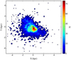 |
Fig. 2. Same as Fig. 1 but for the SMC. |
| In the text | |
|
Fig. 3. Left panels: P–L diagrams in the LMC for the FU and FO Cepheids. Right panels: combined FU and FO Cepheids after converting the period of FO Cepheids to corresponding periods of FU Cepheids. Upper panels: V filter. Lower panels: I filter. Blue and red points are for FU and FO Cepheids, respectively. |
| In the text | |
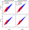 |
Fig. 4. Same as Fig. 3 but for the SMC. |
| In the text | |
|
Fig. 5. P–L relations for a sub-region in the LMC in the V band (upper panel) and I band (lower panel). Here, the continuous lines represent the best linear fit with a fixed slope of −2.769 for the V band and −2.961 for the I band, respectively. The dashed lines represent the 3σ cut lines and Cepheids outside 3σ lines are shown by open circles which are not considered in the best fit. |
| In the text | |
|
Fig. 6. Histogram of reddening values in 133 segments of the LMC shown by continuous line. The dashed line represents the best fit with a log-normal distribution. |
| In the text | |
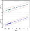 |
Fig. 7. Same as Fig. 5 but for the SMC with a fixed slope of −2.66 for V band and −2.918 for I band. |
| In the text | |
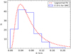 |
Fig. 8. Same as Fig. 6 but for the 136 segments of the SMC. |
| In the text | |
|
Fig. 9. Reddening maps emanating from the P–L diagrams of the Cepheids in the LMC. North is up and east is to the left. The optical centre of the LMC is shown by a plus symbol. The colour bar represents the interpolated reddening E(V − I). |
| In the text | |
|
Fig. 10. Upper panel: distribution of the ΔE(V − I), i.e. the results of past studies subtracted from our results in the LMC as mentioned in the top-left corner. Lower panel: difference ΔE(B − V) between our reddening estimates and those of Inno et al. (2016). |
| In the text | |
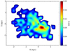 |
Fig. 11. Same as Fig. 9 but for the SMC. |
| In the text | |
|
Fig. 12. Upper panel: distributions of ΔE(V − I), i.e. past reddening estimates subtracted from our estimate in the SMC as mentioned in the top-left corner. Lower panel: difference of E(B − V) from Rubele et al. (2018) subtracted from our reddening estimate. |
| In the text | |
|
Fig. 13. Lower panel: histogram of the difference Δ E(V − I) between the present study and those of Udalski et al. (1999) shown by a continuous line, and Sandage et al. (2004) shown by a dashed line. Upper panel: heat map representing the difference in reddening divided by reddening uncertainty in each segment, left panel – between the present reddening estimates and those of Udalski et al. (1999); right panel – between the present reddening estimates and those of Sandage et al. (2004). The difference is obtained by subtracting the results of other studies from our estimates. |
| In the text | |
|
Fig. 14. Same as Fig. 13 but for the SMC. Here, comparisons are made between our maps and those obtained by Udalski et al. (1999) and Sandage et al. (2009) using P–L relations. |
| In the text | |
|
Fig. 15. Age distribution of Cepheids in the LMC. The best-fit Gaussian profile is shown by a dashed red line. |
| In the text | |
|
Fig. 16. Same as Fig. 15 but for the SMC. The best-fit double-Gaussian profile is shown by a dashed red line and the individual Gaussian is shown as a dotted green line. |
| In the text | |
|
Fig. 17. Spatial distributions of the Cepheids in the 389 segments of the LMC as a function of their mean log(t/yr). North is up and east is to the left. The location of the optical centre of the LMC is shown by a plus symbol. |
| In the text | |
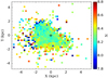 |
Fig. 18. Same as Fig. 17 but for the 562 segments in the SMC. |
| In the text | |
Current usage metrics show cumulative count of Article Views (full-text article views including HTML views, PDF and ePub downloads, according to the available data) and Abstracts Views on Vision4Press platform.
Data correspond to usage on the plateform after 2015. The current usage metrics is available 48-96 hours after online publication and is updated daily on week days.
Initial download of the metrics may take a while.