| Issue |
A&A
Volume 627, July 2019
|
|
|---|---|---|
| Article Number | A8 | |
| Number of page(s) | 9 | |
| Section | The Sun | |
| DOI | https://doi.org/10.1051/0004-6361/201834163 | |
| Published online | 25 June 2019 | |
Estimating the mass of CMEs from the analysis of EUV dimmings
1
Instituto de Ciencias Astronómicas de la Tierra y del Espacio (ICATE-CONICET), Av. España Sur 1512, CC 49, 5400 San Juan, Argentina
e-mail: This email address is being protected from spambots. You need JavaScript enabled to view it.
, This email address is being protected from spambots. You need JavaScript enabled to view it.
2
Facultad de Ciencias Exactas, Físicas y Naturales, Universidad Nacional de San Juan, Av. José Ignacio de la Roza Oeste 590, J5402DCS San Juan, Argentina
3
Universidad Tecnológica Nacional – Facultad Regional Mendoza, CONICET, CEDS, Rodriguez 243, 5500 Mendoza, Argentina
4
George Mason University, Fairfax, VA 22030, USA
5
Instituto de Astronomía y Física del Espacio (IAFE, CONICET-UBA), CC 67 – Suc 28, (C1428ZAA) Ciudad Autónoma de Buenos Aires, Argentina
6
Universidad Nacional de Tres de Febrero (UNTREF), Valentín Gómez 4752, Caseros (B1678ABH), Provincia de Buenos Aires, Argentina
Received:
30
August
2018
Accepted:
20
May
2019
Abstract
Context. Reliable estimates of the mass of coronal mass ejections (CMEs) are required to quantify their energy and predict how they affect space weather. When a CME propagates near the observer’s line of sight, these tasks involve considerable errors, which motivated us to develop alternative means for estimating the CME mass.
Aims. We aim at further developing and testing a method that allows estimating the mass of CMEs that propagate approximately along the observer’s line of sight.
Methods. We analyzed the temporal evolution of the mass of 32 white-light CMEs propagating across heliocentric heights of 2.5–15 R⊙, in combination with that of the mass evacuated from the associated low coronal dimming regions. The mass of the white-light CMEs was determined through existing methods, while the mass evacuated by each CME in the low corona was estimated using a recently developed technique that analyzes the dimming in extreme-UV (EUV) images. The combined white-light and EUV analyses allow the quantification of an empirical function that describes the evolution of CME mass with height.
Results. The analysis of 32 events yielded reliable estimates of the masses of front-side CMEs. We quantified the success of the method by calculating the relative error with respect to the mass of CMEs determined from white-light STEREO data, where the CMEs propagate close to the plane of sky. The median for the relative error in absolute values is ≈30%; 75% of the events in our sample have an absolute relative error smaller than 51%. The sources of uncertainty include the lack of knowledge of piled-up material, subsequent additional mass supply from the dimming region, and limitations in the mass-loss estimation from EUV data. The proposed method does not rely on assumptions of CME size or distance to the observer’s plane of sky and is solely based on the determination of the mass that is evacuated in the low corona. It therefore represents a valuable tool for estimating the mass of Earth-directed events.
Key words: Sun: activity / Sun: corona / Sun: coronal mass ejections (CMEs)
© ESO 2019
1. Introduction
Coronal mass ejections (CMEs) are one of the most spectacular transient events observed in the solar atmosphere. They propagate in the interplanetary medium, where under certain conditions, Earth-directed CMEs can perturb the environment of our planet, producing intense geomagnetic storms. The analysis of CMEs has mostly been performed by means of white-light coronagraph images, which have enabled the estimation of their mass on the basis of the Thomson scattering formulation (Billings 1966). Vourlidas et al. (2000) studied mass and energy of a sample of CMEs using data from the Large Angle and Spectrometric Coronagraph (LASCO; Brueckner et al. 1995) on board the Solar and Heliospheric Observatory (SOHO).
More recent efforts (e.g., Colaninno & Vourlidas 2009) profited from the multiple viewpoints provided by the coronagraphs from the Sun Earth Connection Coronal and Heliospheric Investigation (SECCHI; Howard et al. 2008) on board the Solar Terrestial Relations Observatory (STEREO) to obtain a more accurate determination of the mass of CMEs. Vourlidas et al. (2010) investigated the effect in the calculation of the CME mass on two dominating sources of uncertainty, namely the determination of its propagation angle relative to the plane of sky (POS), and the unknown 3D distribution of its mass. At high propagation angles with respect to the POS, the Thomson scattering drastically drops, which increases the uncertainties in the mass determinations. This is the case for Earth-directed CMEs that propagate at a high angle with respect to the POS of a coronagraph located on the Sun-Earth line. For such events the mass of the CME can be underestimated by up to 70% under the assumption of propagation along the POS, and overestimated by up to 500% if the correction for the propagation angle is considered (Vourlidas et al. 2010). Furthermore, under these circumstances, the coronagraph occulter blocks out a significant amount of the Earth-directed mass. These limitations and the possibility of not having space-borne coronagraph observations from different vantage points in the near future, urge for the conception of a different approach for estimating the mass of Earth-directed events.
The need for accurate estimates of the mass of CMEs is justified for different applications. Particularly for space weather modeling, the mass of the CME is a fundamental parameter playing a key role in the determination of energetics. Falkenberg et al. (2010) identified the CME cloud density as one of the most important parameters required to predict the physical characteristics of interplanetary CMEs (ICMEs) near Earth’s environment in a realistic way. Similarly, Kay et al. (2015) showed that the CME propagation profile is highly sensitive to the mass that is assumed. Moreover, accurate estimates of the mass of CMEs and its time-evolution are required for predicting their in situ measured magnetic field profiles, as shown by Kay & Gopalswamy (2017). These estimates generally rely on the values provided by the Coordinated Data Analysis Worskshops (CDAW) CME catalog using LASCO observations. Accurate values of CME kinetic energies are also key to determine the efficiency of CME shocks in accelerating solar energetic particles, as done by Mewaldt et al. (2005, 2008). Another important disturbance of the Earth’s environment includes the compression of the magnetosphere as a result of higher momentum flux, that is, high density and velocity, causing geomagnetically induced currents (GICs). Using density measurements from the coronagraphs on board STEREO, Savani et al. (2013) concluded that the momentum flux of a CME plays a key role in forecasting the occurrence of GICs at Earth.
The discovery of transient depletions in the low corona in extreme-ultraviolet (EUV) and soft X-ray wavelengths (Rust & Hildner 1976; Hudson & Lemen 1998; Zarro et al. 1999; Harrison & Lyons 2000; Harrison et al. 2003) led to speculate that these coronal dimmings are closely related with the eruption of CMEs. Several studies have analyzed the relationship between mass loss from dimming regions and the mass of the associated CMEs determined from white-light data (e.g., Harrison et al. 2003; Aschwanden et al. 2009; Aschwanden & Boerner 2011; Tian et al. 2012; López et al. 2017), usually considering that dimmings are located at the footpoints of the corresponding CMEs (Thompson et al. 2000). Recently, López et al. (2017) investigated the time evolution of the evacuated mass in the dimming and compared it with the evolution of the mass of the associated CME observed in white light. They found that the time evolution of the mass loss at the dimming is characterized by a rapid rise phase followed by a leveling off. After the analysis of three events, they suggested that the CME mass could be inferred from the mass loss determined from EUV images. This mass-loss estimation represents at least a lower limit for the mass of a CME. This is mainly because not all the material that constitutes these events arises from the low corona. The core of CMEs is mostly composed of chromospheric material of an eruptive filament, while their leading edge also piles up coronal material during its propagation through the corona. Therefore these contributions cannot be addressed by only quantifying mass loss in EUV dimmings (henceforth referred to as EUV mass loss). Instead, they require a combined analysis of EUV mass loss and the mass of the associated CMEs in white light.
The main objective of this study is to determine the CME mass from EUV mass-loss measurements. This is of particular importance for Earth-directed CMEs whose mass estimates are highly inaccurate (Vourlidas et al. 2000, 2010). By combining the analyses of EUV mass loss and the CME mass evolution in white-light images, we propose an empirical method for estimating the evolution of CME mass as a function of height. The method requires only measurements of mass evacuated from the associated dimmings, and results in a suitable alternative to estimating the mass of front-side CMEs (i.e., when Thomson scattering is least efficient).
The manuscript is organized as follows. Section 2 presents the methodology used to estimate the mass evacuated in dimming regions from EUV data, as well as the mass of the associated CMEs measured in coronagraph white-light data. Section 3 presents the application of the method developed by Bein et al. (2013) to simultaneously characterize the evolution of the CME mass as determined from white-light data and the evolution of the mass loss derived from EUV images. Section 4 outlines the methodology proposed to predict the evolution of CME mass from EUV observations. Finally, Sect. 5 presents the summary and conclusions of the work.
2. Estimation of mass from EUV and white-light images
We analyze 32 events identified in images provided by the Atmospheric Imaging Assembly (AIA, Lemen et al. 2012) on board the Solar Dynamics Observatory (SDO) and COR2 on board STEREO. All of them present an on-disk dimming detected in EUV images of the low corona and an associated CME observed in the white-light corona. The EUV dimmings analyzed in this work are assumed to be caused by the eruption of material from the low corona that can be related to CMEs observed in white light. The coronal mass evacuated by the eruption is derived from a differential emission measure (DEM) analysis. As discussed in López et al. (2017), the use of three EUV narrowbands to estimate the DEM, as well as the definition of the dimming region based in a density analysis instead of using a single EUV passband, discard mechanisms other than mass loss (Mason et al. 2014) to explain the occurrence of the analyzed dimmings. Furthermore, a number of past studies have interpreted coronal dimmings as density depletions due to mass loss or rapid expansion of the overlying corona (e.g., Hudson & Lemen 1998; Thompson et al. 2000; Harrison & Lyons 2000; Harrison et al. 2003; Zhukov & Auchère 2004) rather than as other mechanisms.
The events occurred between 23 May 2010 and 17 April 2012 when the STEREO spacecraft were nearly in quadrature with respect to the Sun-Earth direction. In this work, we selected events for which the CME and dimming can be associated in an unambiguous fashion, as discussed below. A considerably larger sample of events is required for a statistically meaningful representation of the association of dimmings and CMEs for the full possible spectrum of events. A detailed analysis of such a sample is beyond the scope of the present effort.
The selection of events was restricted with the following criteria. We first checked the COR2 data in order to find bright and clear CMEs, that is, excluding poor events. Then, we identified their source regions and sought for the presence of a related dimming. In order to avoid dimmings observed near the limb from Earth’s perspective, only events associated with source regions located between [−50°,+50°] heliographic longitude were selected. This consideration reduces projection effects when determining the area of the dimming regions, but increases the possibility that the direction of propagation of the associated CME is close to the POS for at least one of the STEREO spacecraft. The latter reduces uncertainties in the quantification of CME parameters. Events for which the COR2 coronagraph images showed multiple CMEs were dismissed. We selected only events that permitted us to unambiguously identify their associated source regions.
The selected events are summarized in Table 1. The first columns of Table 1 display (1) an identification number for each event, (2) the date and (3) start time of the eruptive events in the low corona, (4) the heliographic coordinates of the eruption site, and (5) the X-ray flare class. For events associated with an X-ray flare, the start time and heliographic coordinates correspond to those provided by the Geostationary Operational Environmental Satellite (GOES) and/or the X-Ray Telescope (XRT, Watanabe et al. 2012) catalogs. For events not associated with a flare registered by any of the two catalogs, the start time and the location of the eruption were estimated from visual inspection of AIA images.
Main properties of the analyzed events and their predicted mass.
As a starting point, we independently estimated the temporal evolution of the mass evacuated from the dimming regions and the evolution of the mass of the associated CMEs in white light. The mass loss from the dimming regions was determined by applying the DEM technique on AIA data, as described in detail in López et al. (2017) and Nuevo et al. (2015). The DEM was constructed for the passbands of AIA centered at 171 Å (Fe IX), 193 Å (Fe XII/Fe XXIV), and 211 Å (Fe XIV). Hereafter, we refer to the mass loss estimated from the EUV dimming regions as MEUV. The error of the mass estimated from the DEM analysis of the EUV dimming is 25%. This is on the order of the uncertainty of the absolute radiometric calibration of the AIA data after all data-processing and (time-dependent) correction procedures provided by the AIA team in the SolarSoft package were applied (Boerner et al. 2014; Boerner, priv. comm.).
The mass of the associated CMEs is determined from total-brightness images provided by the COR2 coronagraph on board STEREO. The spacecraft used in each case to estimate the mass in white light is indicated in Col. (6) of Table 1. The mass was calculated following the method described by Vourlidas et al. (2010) and applying the correction by the propagation angle of the CMEs with respect to the POS of the instrument (ω, Col. 7 in Table 1). To estimate the three-dimensional direction of propagation of the CMEs, we used the graduated cylindrical shell (GCS) model (Thernisien et al. 2009). The model was simultaneously applied to COR2-A, COR2-B, and LASCO C2 images, at a time when the CME was seen fully developed in the field of view (FOV) of the three coronagraphs. A detailed description of the full methodology is provided by López et al. (2017). For events 11, 28, and 31, it was not possible to obtain a good fit of the model to the observed CME. The propagation direction considered in these cases are the coordinates of the associated eruption, that is, assuming that the CMEs propagate radially from the eruption site. The CME mass values determined in this way from COR2 white-light data are called MCOR2 here. Following the analysis described in Bein et al. (2013), we adopted an error of ±15% for the MCOR2 CME mass measurements. This error accounts for uncertainties arising from the presence of coronal structures in the region of interest that are not related to the CME, and for errors related to the pre-event image subtraction. For completeness, Cols. (8) and (9) in Table 1 display the angular width (AW) of the CMEs deduced from the GCS model and the CME speed at 10 R⊙ obtained from a second-order fit to the COR1 and COR2 deprojected height estimates. For events 11, 28, and 31, the AW was taken from the Computer Aided CME Tracking software (CACTus, Robbrecht & Berghmans 2004).
3. Evolution of mass estimated from EUV and white-light data: Implementation of the technique
To describe the height evolution of CME-associated mass, we used the expressions presented by Bein et al. (2013) that were later applied by Feng et al. (2015). They describe the evolution of the mass of a CME MCME (determined from white-light data) as a function of the height h of the leading edge:
 (1)
(1)
where m0 is the initial ejected mass, Δm is the mass increase per unit height during the propagation of the CME in the FOV of the coronagraph, and hc is the height for which it is verified that MCME(h = hc)=0. Although Bein et al. (2013) defined hc as the effective occultation size, this definition lacks meaning in the context of our analysis because we also include data values corresponding to low coronal heights, as explained below.
The mass evolution as derived from COR2 images shows a significant increase (see, e.g., the asterisks in Fig. 1). This is particularly noticeable in the range of heliocentric heights up to 8 R⊙, where the CME has not yet fully emerged from behind the occulter. To account for this missing mass behind the occulter, Bein et al. (2013) proposed the following correction:
 (2)
(2)
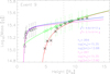 |
Fig. 1. EUV mass loss (MEUV, triangles) and CME mass determined from COR2 white-light data (MCOR2, asterisks) values. The red curve shows the fit through all MCOR2 values. The blue curve is the fit through all MEUV values and MCOR2 values with h ≥ 8 R⊙. The diamonds indicate the MCOR2 values corrected by the occulter effect. The green curve is the fit yielded by Eq. (2) through these corrected values. The magenta curve is the fit through the corrected CME mass values and the MEUV mass-loss points. The vertical dashed line marks h = 8 R⊙. |
In the case of COR2, the effect of the occulter can be ignored in most of the cases, when the height of the leading edge of the CME is larger than ≈ 8 R⊙ (Feng et al. 2015).
The mass-related nomenclature used here is the following:
-
MEUV: mass loss estimated from the dimming regions using EUV data (triangles in Fig. 1, described below).
-
MCOR2: mass of the CMEs directly measured from COR2 white-light data (asterisks in Fig. 1).
-
MWL: the corresponding MCOR2 value at 10 R⊙.
We used Eqs. (1) and (2) to fit both the CME mass estimated from the COR2 white-light data and the mass loss in the low corona estimated from the AIA EUV data. Figure 1 shows these two quantities as a function of the deprojected height of the CME leading edge, measured at the central position angle. These deprojected heights arise from correcting the height measurements performed in the COR1 and COR2 FOVs by the propagation angle ω. The triangles indicate the mass loss (MEUV) in the coronal dimming region (every 10 min, determined as explained in Sect. 2) as a function of the deprojected CME height in the FOV of COR1 (h ≤ 4 R⊙). It is expected that when the CME has reached 4 R⊙, most of the mass evacuation has taken place, although some material continues to be evacuated at a lower rate (López et al. 2017). The maximum height at which it was possible to unambiguously measure the CME leading edge in COR1 is shown in Col. (10) of Table 1, while the MEUV value displayed in Col. (11) corresponds to the time of that height measurement (i.e., the last triangle). The asterisks in Fig. 1 represent the mass values of the CME determined from white-light data (MCOR2) as a function of the respective deprojected height of its leading edge, both quantities measured in the FOV of COR2. The CME mass as measured from white-light images at 10 R⊙ (MWL, shown in Col. 12 of Table 1) is estimated by fitting Eq. (1) to the MCOR2 values (asterisks in Fig. 1).
The blue solid curve in Fig. 1 indicates the fit yielded by Eq. (1) using the mass-loss (MEUV, triangles) and CME mass (MCOR2, asterisks) values. Only the points corresponding to MCOR2 measured at distances larger than 8 R⊙ are taken into account. At these distances, the effect of the occulter in the determination of mass becomes negligible.
The diamonds in Fig. 1 are the values of MCOR2 corrected by the occulter effect using Eq. (2). The green solid curve represents the fit through these corrected mass-height points. The parameters (m0, Δm, hc) are considered free, and their initial values are taken from the fit of Eq. (1) only to the MCOR2 values (red curve in Fig. 1). The free parameters are then modified using a nonlinear least squares fit. Finally, the magenta curve corresponds to Eq. (1) using the mass-loss values (MEUV, triangles) and all CME mass values corrected using Eq. (2) (diamonds).
In Eq. (1), used for the blue and magenta fits, the following conditions were considered: the value of m0 was fixed, while the parameters hc and Δm were free and were iteratively modified using a nonlinear least squares fit. The value of m0, defined as a lower limit of CME mass, is the mass loss value MEUV in Col. (11) of Table 1. The blue and magenta curves in Fig. 1 represent the fitting functions for the masses uncorrected and corrected for the occulter effect (hereafter uncorrected and corrected), respectively. The mass values at 10 R⊙ resulting from the uncorrected (Mu) and corrected (Mc) fits are shown in Cols. (13) and (14) of Table 1. To evaluate the goodness of fits to the measured mass values for the uncorrected and corrected analyses, we computed the value of chi-square goodness using the following expression:  . Where N is the number of points to fit, Mmea is the mass measured using white-light or EUV data, and Mfit is the mass obtained from the corresponding fit function.
The procedure described above, shown in Fig. 1 for event 9, was applied to 25 of 32 events of the sample. The corresponding plots for the other eight events are shown in Fig. 2. For seven events, it was not possible to use the method for various reasons (see Sect. 4.1).
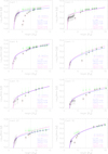 |
Fig. 2. Same as Fig. 1 for event 9, but for the other eight analyzed events. Red and green fits are not shown in the plots. Event numbers correspond to the identification given in Table 1. |
The frequency of the hc and Δm values resulting from the implementation of the technique that describes mass evolution in 25 events is displayed in Fig. 3. The top row corresponds to values resulting from the fits through white-light points uncorrected by the occulter effect and the bottom row to those corrected by this effect. The distributions show a significant concentration around the mean values.
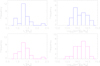 |
Fig. 3. Histograms of the parameters hc and Δm obtained for the uncorrected (upper row) and corrected (lower row) cases. |
4. Method for predicting the CME mass
After the fit functions were applied to 25 events of the sample, the next step was to develop a tool for predicting the CME mass on the basis of the evacuated mass from the associated dimmings. We used Eq. (1) considering hc and Δm as fixed parameters, resulting from their average after the fitting of 25 events. As shown earlier (Fig. 3), the dispersion of these parameters is small enough to use mean values as input to the prediction method. The mean values of  and
and  are shown in Table 2, with i = [u, c] for the uncorrected or corrected masses, respectively.
Mean values ( and
and  ) of the parameters
  and Δmi for the analyses performed using the assumptions that are uncorrected and corrected for the occulter effect.
Based on Eq. (1), the mass of a CME as a function of the height h of its leading edge for heliocentric distances up to 15 R⊙ can be estimated as
 (3)
(3)
where i = [u, c] indicates the values uncorrected or corrected for the occulter effect. Here we use the following nomenclature:
-
 : mass of the CME predicted with our method without correcting for the occulter effect.
 -
 : mass of the CME predicted with our method including the correction for the occulter effect.
Equation (3) only requires a single value of the evacuated mass MEUV from the associated dimming region as input. For these 25 events, we used the last value of the mass loss in the dimming region (last triangle). The predicted mass values  and
and  at h = 10 R⊙ for the analyzed CMEs using Eq. (3) are shown in Cols. (15) and (17) in Table 1.
Figure 4 compares the CME masses predicted by Eq. (3) ( ) versus the CME masses estimated from the white-light measurements (MWL). The latter is directly obtained from the mass of the CME measured in COR2 images for events propagating on or very close to the POS of the instrument. Therefore the values can be regarded as close to the true mass of a CME. Filled symbols are addressed in Sect. 4.1.
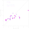 |
Fig. 4. Mass of the CMEs predicted by the method (Mpred) vs. the CME mass determined from white-light data (MWL) for the 32 analyzed events at 10 R⊙. Blue circles represent masses predicted without applying the correction by the occulter effect, while magenta squares show the masses after the correction is applied. The filled symbols correspond to the events for which we could not apply the technique (see Sect. 4.1). The dotted straight line represents the identity line (Mpred = MWL). The correlation coefficients and the errors σpred of the predicted mass at 10 R⊙ are shown. |
4.1. Sample predictions to test the performance of the method
As mentioned in Sect. 3, it was not possible to fit the full mass evolution to seven events because of diverse reasons, such as a gap in COR1 data, only few measurements for the fastest CMEs, or mass-loss estimations possible after the front of the CME left the FOV of COR1. Therefore, the hc and Δm parameters could not be deduced for these cases (events with empty values in Cols. 13 and 14). However, it is still possible to test the performance of the CME mass prediction method proposed above on these seven events. For these events the input value (MEUV) in Eq. (3) is the maximum of the mass-loss value from the associated dimming region. An example of the corrected and uncorrected versions of the prediction method is displayed in Fig. 5 (blue and magenta squares). The mass of the CME in white light at COR2 heights is also shown as asterisks for comparison. The predicted mass of the CMEs for the seven events are included in Cols. (15) and (17) in Table 1, while the corresponding values are also included in Fig. 4, but as filled symbols. The predicted masses for the events in our test sample fall within the full set of events, with only one exception.
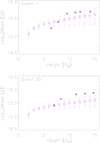 |
Fig. 5. Evolution of the measured and predicted mass of the CMEs for events 7 and 30 as a function of height. The CME mass measured from COR2 white-light data is indicated by asterisks. The mass predicted by Eq. (3) is indicated by blue squares for the analysis based on uncorrected data and by magenta triangles for the analysis based on corrected data. |
4.2. Validation of the prediction method
To validate our method, we further calculated the relative error ( ) of the mass predicted by Eq. (3) (
 ) with respect to the measured CME mass using COR2 images near quadrature (MWL). Although MWL is not the actual CME mass value, it is accepted as a good proxy after the methodology described in Sect. 2.
 (4)
(4)
The relative errors for the 32 events, ( ) and (
 ) are also included in Table 1, in Cols. (16) and (18), respectively. The frequency of the absolute value of the relative error
  resulting from Eq. (4) is shown in Fig. 6 as histograms for the estimates that are based on masses that were not corrected for the occulter effect (Fig. 6 left), and for those corrected for the occulter effect (Fig. 6 right). The median value in the relative errors is of 30%. It is important to mention that for the events in the test sample that we discussed in the previous section, the errors are smaller than 52% for 5 out of 7 events.
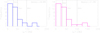 |
Fig. 6. Histograms of the relative error in absolute value of the prediction of CME masses for the 32 events using Eq. (3). Left: absolute value of the relative errors of the CME mass estimation using the parameters from the fitting functions for the uncorrected case (Col. 16 of Table 1). Right: same for the corrected case (Col. 18 of Table 1). The vertical dotted lines indicate the 50th, 75th, and 90th percentiles. |
We further assessed whether the analysis performed using the correction for the occulter effect results (or does not) in a better estimate of CME masses through Eq. (3). For this, we determined the root mean squared error ( ), which is given by the following expression:
where i = [u, c] denotes whether uncorrected or corrected masses were used, j identifies the event, n = 32 is the total number of events,  are the values of the CME masses predicted by Eq. (3), and MWL, j is the CME mass estimated from white-light data at 10 R⊙ for event j. The resulting values are
  and
and  for the uncorrected and the corrected sets of values, respectively.
5. Discussion and conclusions
We applied the DEM technique to AIA images to estimate the mass loss from the EUV low corona due to CMEs for 32 events presenting a coronal dimming and an associated CME. Additionally, using data obtained by COR2 nearly in quadrature with the Sun-Earth direction, we estimated the mass evolution of the respective CMEs from white-light data. Mass values deduced from white-light data were also corrected for the blocking effect of the occulter.
For 25 out of 32 events, we analyzed the combined evolution of the mass-loss profiles from the dimming regions and the mass profiles of the associated CMEs determined from white-light data as a function of the height of the CME fronts measured in the FOV of COR1 and COR2. We then adapted the expression presented by Bein et al. (2013) to predict the mass of CMEs as a function of the heliocentric height of the leading edge.
To quantify the success of the technique, we compared the mass predicted using the proposed methodology with the CME masses measured in the COR2 images. Our analysis indicates that the median of the relative error in absolute value between the masses predicted by our method (Mpred) and those obtained from measurements in white-light data (MWL) is ≈30%, both when the occulter effect is accounted for and when it is not. Furthermore, this relative difference ranges within ±50% for 24 out of 32 events for the uncorrected and corrected cases, respectively, as shown by the percentiles indicated in Fig. 6. In agreement with these results, we found that for the 75% of the totality of the events, the relative errors in absolute value between predicted and measured CME masses are lower than 51.1% (uncorrected) and 50.4% (corrected).
The analysis of the RMSE indicates that the correction for the occulter effect to the measured masses of the CMEs in white light does not provide a substantial improvement in the estimation of the mass. The same conclusion can be drawn from Fig. 6, where the histograms of the relative errors show a similar appearance in both cases.
An improvement in the estimation of CME masses with the method proposed here requires a better understanding of the mass increase term (Δm). This contribution to the evolution of the mass of a CME includes two main components: (a) the pile-up of plasma at the front of the CME during its propagation, and (b) the further evacuation of mass from the lower corona at the dimming region. In this regard, Feng et al. (2015) studied the mass increase due to the interaction of CMEs with the ambient solar wind for six events. They found that the solar wind pile-up plays an important role in the mass increase of the CMEs. However, for two-thirds of the events, they could not fully explain the mass increase by means of the pile-up model. They proposed that evacuation of mass from the associated dimmings in the low corona may explain this controversy. In a recent study, Howard & Vourlidas (2018) analyzed the volume electron density evolution of the fronts of 13 three-part CMEs. They found no evidence for pile-up at the front of the CMEs from 2.6–30 R⊙. They argued that pile-up takes place during the propagation of the CME in the low corona.
By comparing the mass-loss evolution profiles in dimming regions with the height evolution of the associated CMEs, López et al. (2017) found evidence that although most of the evacuation takes place while the CMEs propagate during the first four solar radii, some evacuation is still ongoing while the CMEs propagate in the FOV of COR2. This suggests that the evacuation process remains active even when the leading edge has already reached several solar radii of heliocentric distance, likely adding mass to the CME in conjunction with the pile-up process.
Furthermore, a dominant source of uncertainty comes from the nature of the methodology used here to estimate MEUV. As indicated in López et al. (2017), the mass determined as evacuated from the dimming regions is underestimated. Particularly, hot plasma (T ≥ 2.5 MK) is not considered in the mass-loss estimation, while the eruptive filament and the post-eruptive loops covering the dimming region during the pre-event and post-event times may also affect the calculation.
The work presented here applies to dimmings produced by mass evacuation. Further studies are necessary to confirm whether different parameters in the empirical relation are needed for different dimming signatures and/or different eruption scenarios. Furthermore, additional investigation is necessary to achieve a better understanding on the pile-up of material during CME evolution in the low corona and to determine the contribution from mass loss in dimming regions. These are still fundamental open questions that need to be answered to unveil the nature of the CME mass evolution in the corona and inner heliosphere. Nonetheless, the novel technique proposed in this work results in a feasible tool for extrapolating the mass of CMEs in the inner heliosphere from the EUV mass loss in the associated dimming regions. This is very important in the absence of coronagraph images from multiple views and in the case of front-side events, where the uncertainties in the CME mass determined using white-light coronagraphs located along the direction of propagation yield unreliable results.
Acknowledgments
The authors acknowledge support from the Universidad Tecnológica Nacional (UTN) grant UTI4035TC, and the Agencia Nacional de Promoción Científica y Tecnológica (ANPCyT) grant 2012-0973. FML and FAN are fellows of CONICET. HC and AMV are members of the Carrera del Investigador Científico (CONICET). The authors acknowledge the use of data from the STEREO (NASA), SDO (NASA), and SOHO (ESA/NASA) missions. These data are produced by the AIA, HMI, SECCHI, LASCO, and MDI international consortia.
References
- Aschwanden, M. J., & Boerner, P. 2011, ApJ, 732, 81 [NASA ADS] [CrossRef] [Google Scholar]
- Aschwanden, M. J., Nitta, N. V., Wuelser, J.-P., et al. 2009, ApJ, 706, 376 [NASA ADS] [CrossRef] [Google Scholar]
- Bein, B. M., Temmer, M., Vourlidas, A., Veronig, A. M., & Utz, D. 2013, ApJ, 768, 31 [Google Scholar]
- Billings, D. E. 1966, A Guide to the Solar Corona (New York: Academic Press) [Google Scholar]
- Boerner, P. F., Testa, P., Warren, H., Weber, M. A., & Schrijver, C. J. 2014, Sol. Phys., 289, 2377 [NASA ADS] [CrossRef] [Google Scholar]
- Brueckner, G. E., Howard, R. A., Koomen, M. J., et al. 1995, Sol. Phys., 162, 357 [NASA ADS] [CrossRef] [Google Scholar]
- Colaninno, R. C., & Vourlidas, A. 2009, ApJ, 698, 852 [Google Scholar]
- Falkenberg, T. V., Vršnak, B., Taktakishvili, A., et al. 2010, Space Weather, 8, S06004 [NASA ADS] [CrossRef] [Google Scholar]
- Feng, L., Wang, Y., Shen, F., et al. 2015, ApJ, 812, 70 [Google Scholar]
- Harrison, R. A., & Lyons, M. 2000, A&A, 358, 1097 [NASA ADS] [Google Scholar]
- Harrison, R. A., Bryans, P., Simnett, G. M., & Lyons, M. 2003, A&A, 400, 1071 [NASA ADS] [CrossRef] [EDP Sciences] [Google Scholar]
- Howard, R. A., & Vourlidas, A. 2018, Sol. Phys., 293, 55 [NASA ADS] [CrossRef] [Google Scholar]
- Howard, R. A., Moses, J. D., Vourlidas, A., et al. 2008, Space Sci. Rev., 136, 67 [NASA ADS] [CrossRef] [Google Scholar]
- Hudson, H. S., Lemen, J. R., & St. Cyr, O. C., Sterling, A. C., & Webb, D. F., 1998, Res. Lett., 25, 2481 [NASA ADS] [CrossRef] [Google Scholar]
- Kay, C., & Gopalswamy, N. 2017, J. Geophys. Res. (Space Phys.), 122, 11 [Google Scholar]
- Kay, C., dos Santos, L. F. G., & Opher, M. 2015, ApJ, 801, L21 [NASA ADS] [CrossRef] [Google Scholar]
- Lemen, J. R., Title, A. M., Akin, D. J., et al. 2012, Sol. Phys., 275, 17 [NASA ADS] [CrossRef] [Google Scholar]
- López, F. M., Hebe Cremades, M., Nuevo, F. A., Balmaceda, L. A., & Vásquez, A. M. 2017, Sol. Phys., 292, 6 [NASA ADS] [CrossRef] [Google Scholar]
- Mason, J. P., Woods, T. N., Caspi, A., Thompson, B. J., & Hock, R. A. 2014, ApJ, 789, 61 [Google Scholar]
- Mewaldt, R. A., Cohen, C. M. S., Mason, G. M., et al. 2005, in Solar Wind 11/SOHO 16, Connecting Sun and Heliosphere, eds. B. Fleck, T. H. Zurbuchen, & H. Lacoste, ESA SP, 592, 67 [NASA ADS] [Google Scholar]
- Mewaldt, R. A., Cohen, C. M. S., Giacalone, J., et al. 2008, in AIP Conf. Ser., eds. G. Li, Q. Hu, O. Verkhoglyadova, et al., 1039, 111 [NASA ADS] [CrossRef] [Google Scholar]
- Nuevo, F. A., Vásquez, A. M., Landi, E., & Frazin, R. 2015, ApJ, 811, 128 [NASA ADS] [CrossRef] [Google Scholar]
- Robbrecht, E., & Berghmans, D. 2004, A&A, 425, 1097 [NASA ADS] [CrossRef] [EDP Sciences] [Google Scholar]
- Rust, D. M., & Hildner, E. 1976, Sol. Phys., 48, 381 [NASA ADS] [CrossRef] [Google Scholar]
- Savani, N. P., Vourlidas, A., Pulkkinen, A., et al. 2013, Space Weather, 11, 245 [NASA ADS] [CrossRef] [Google Scholar]
- Thernisien, A., Vourlidas, A., & Howard, R. A. 2009, Sol. Phys., 256, 111 [Google Scholar]
- Thompson, B. J., Cliver, E. W., Nitta, N., Delannée, C., & Delaboudinière, J.-P. 2000, Geophys. Res. Lett., 27, 1431 [Google Scholar]
- Tian, H., McIntosh, S. W., Xia, L., He, J., & Wang, X. 2012, ApJ, 748, 106 [Google Scholar]
- Vourlidas, A., Subramanian, P., Dere, K. P., & Howard, R. A. 2000, ApJ, 534, 456 [Google Scholar]
- Vourlidas, A., Howard, R. A., Esfandiari, E., et al. 2010, ApJ, 722, 1522 [NASA ADS] [CrossRef] [Google Scholar]
- Watanabe, K., Masuda, S., & Segawa, T. 2012, Sol. Phys., 279, 317 [NASA ADS] [CrossRef] [Google Scholar]
- Zarro, D. M., Sterling, A. C., Thompson, B. J., Hudson, H. S., & Nitta, N. 1999, ApJ, 520, L139 [Google Scholar]
- Zhukov, A. N., & Auchère, F. 2004, A&A, 427, 705 [NASA ADS] [CrossRef] [EDP Sciences] [Google Scholar]
All Tables
Mean values ( and ) of the parameters and Δmi for the analyses performed using the assumptions that are uncorrected and corrected for the occulter effect.
All Figures
|
Fig. 1. EUV mass loss (MEUV, triangles) and CME mass determined from COR2 white-light data (MCOR2, asterisks) values. The red curve shows the fit through all MCOR2 values. The blue curve is the fit through all MEUV values and MCOR2 values with h ≥ 8 R⊙. The diamonds indicate the MCOR2 values corrected by the occulter effect. The green curve is the fit yielded by Eq. (2) through these corrected values. The magenta curve is the fit through the corrected CME mass values and the MEUV mass-loss points. The vertical dashed line marks h = 8 R⊙. |
| In the text | |
|
Fig. 2. Same as Fig. 1 for event 9, but for the other eight analyzed events. Red and green fits are not shown in the plots. Event numbers correspond to the identification given in Table 1. |
| In the text | |
|
Fig. 3. Histograms of the parameters hc and Δm obtained for the uncorrected (upper row) and corrected (lower row) cases. |
| In the text | |
|
Fig. 4. Mass of the CMEs predicted by the method (Mpred) vs. the CME mass determined from white-light data (MWL) for the 32 analyzed events at 10 R⊙. Blue circles represent masses predicted without applying the correction by the occulter effect, while magenta squares show the masses after the correction is applied. The filled symbols correspond to the events for which we could not apply the technique (see Sect. 4.1). The dotted straight line represents the identity line (Mpred = MWL). The correlation coefficients and the errors σpred of the predicted mass at 10 R⊙ are shown. |
| In the text | |
|
Fig. 5. Evolution of the measured and predicted mass of the CMEs for events 7 and 30 as a function of height. The CME mass measured from COR2 white-light data is indicated by asterisks. The mass predicted by Eq. (3) is indicated by blue squares for the analysis based on uncorrected data and by magenta triangles for the analysis based on corrected data. |
| In the text | |
|
Fig. 6. Histograms of the relative error in absolute value of the prediction of CME masses for the 32 events using Eq. (3). Left: absolute value of the relative errors of the CME mass estimation using the parameters from the fitting functions for the uncorrected case (Col. 16 of Table 1). Right: same for the corrected case (Col. 18 of Table 1). The vertical dotted lines indicate the 50th, 75th, and 90th percentiles. |
| In the text | |
Current usage metrics show cumulative count of Article Views (full-text article views including HTML views, PDF and ePub downloads, according to the available data) and Abstracts Views on Vision4Press platform.
Data correspond to usage on the plateform after 2015. The current usage metrics is available 48-96 hours after online publication and is updated daily on week days.
Initial download of the metrics may take a while.