Small dust grain dynamics on adaptive mesh refinement grids

U. Lebreuilly; B. Commerçon; G. Laibe

doi:10.1051/0004-6361/201834147

Home

All issues

Volume 626 (June 2019)

A&A, 626 (2019) A96

Full HTML

Open Access

Issue		A&A Volume 626, June 2019


Article Number		A96
Number of page(s)		17
Section		Numerical methods and codes
DOI		https://doi.org/10.1051/0004-6361/201834147
Published online		19 June 2019

A&A 626, A96 (2019)

I. Methods

U. Lebreuilly, B. Commerçon and G. Laibe

École normale supérieure de Lyon, CRAL, UMR CNRS 5574, Université de Lyon, 46 Allée d Italie, 69364 Lyon Cedex 07, France
e-mail: ugo.lebreuilly@ens-lyon.fr

Received: 28 August 2018
Accepted: 6 May 2019

Abstract

Context. Small dust grains are essential ingredients of star, disk and planet formation.

Aims. We present an Eulerian numerical approach to study small dust grain dynamics in the context of star and protoplanetary disk formation. It is designed for finite volume codes. We use it to investigate dust dynamics during the protostellar collapse.

Methods. We present a method to solve the monofluid equations of gas and dust mixtures with several dust species in the diffusion approximation implemented in the adaptive-mesh-refinement code RAMSES. It uses a finite volume second-order Godunov method with a predictor-corrector MUSCL scheme to estimate the fluxes between the grid cells.

Results. We benchmark our method against six distinct tests, DUSTYADVECT, DUSTYDIFFUSE, DUSTYSHOCK, DUSTYWAVE, SETTLING, and DUSTYCOLLAPSE. We show that the scheme is second-order accurate in space on uniform grids and intermediate between second- and first-order on non-uniform grids. We apply our method on various DUSTYCOLLAPSE simulations of 1 M_⊙ cores composed of gas and dust.

Conclusions. We developed an efficient approach to treat gas and dust dynamics in the diffusion regime on grid-based codes. The canonical tests were successfully passed. In the context of protostellar collapse, we show that dust is less coupled to the gas in the outer regions of the collapse where grains larger than ≃100 μm fall significantly faster than the gas.

Key words: ISM: kinematics and dynamics / hydrodynamics / stars: formation / protoplanetary disks / methods: numerical

© U. Lebreuilly et al. 2019

Open Access article, published by EDP Sciences, under the terms of the Creative Commons Attribution License (http://creativecommons.org/licenses/by/4.0), which permits unrestricted use, distribution, and reproduction in any medium, provided the original work is properly cited.

1. Introduction

Dust grains are thought to represent on average only 1% of the mass of the diffuse interstellar medium (ISM, Mathis et al. 1977; Weingartner & Draine 2001). Their typical size distribution is usually modeled as a power law (Mathis et al. 1977, hereafter MRN). However, recent works indicate that this is probably not the case in the dense parts of the ISM (Pagani et al. 2010; Compiègne et al. 2011; Harsono et al. 2018). In addition, a dynamical size sorting may operate in molecular clouds (Hopkins & Lee 2016; Tricco et al. 2017) or during the protostellar collapse (Bate & Lorén-Aguilar 2017). This sorting leads to important variations in the dust-to-gas ratio, especially for large dust grains.

The dust budget plays an essential role during the star and disk formation processes. On the one hand, it regulates the thermal budget of the medium through its blackbody emission, its absorption, and the photoelectric effect. On the other hand, the charge on the grain surface controls, through their number, the ambipolar, ohmic and hall resistivities during the protostellar collapse (Marchand et al. 2016). Zhao et al. (2016) show that removing grains smaller than ∼100 nm from the dust distribution enhances the effects of ambipolar diffusion, triggering the formation of a rotationally supported disk. As we need to know the dust concentration, a treatment of its dynamics is therefore essential to improve our understanding of stellar, disk, and planet formation.

Bifluid models of strongly coupled dust and gas mixtures are difficult to integrate numerically. For Lagrangian-based methods they tend to produce spurious dust aggregates when the grains are accumulated below the resolution length of the gas (Ayliffe et al. 2012). They also require extremely high spatial resolution in order to capture correctly the dephasing between gas and dust, i.e., the dissipation of energy through the drag (Laibe & Price 2012). Some efficient bifluid treatments were developed to cope with these issues (e.g., semi implicit methods, Lorén-Aguilar & Bate 2014, 2015; Stoyanovskaya et al. 2017, 2018). As an alternative way to model correctly these mixtures, Laibe & Price (2014a) proposed an algorithm for smoothed particle hydrodynamic codes (SPH, Lucy 1977; Gingold & Monaghan 1977) using a monofluid formalism. It has been proven to be efficient in the so-called diffusion approximation valid for strongly coupled mixtures (Price & Laibe 2015). More recently, Hutchison et al. (2018) improved this method and adapted it to treat simultaneously several dust species. Lin & Youdin (2017) and Chen & Lin (2018) have applied the monofluid formalism on a cylindrical grid adapted to protoplanetary disk simulations with an Eulerian approach.

Adaptive mesh refinement (AMR, Berger & Oliger 1984) codes are a complementary approach to SPH in astrophysical or cosmological simulations. Commerçon et al. (2008) show in the context of protostellar collapse that the two methods lead to converged results, but AMR codes capture details more efficiently thanks to the versatility of the refinement criteria. The adaptive mesh is a high performance tool for star formation simulations where a wide range of physical and dynamical scales are considered (e.g., Hennebelle 2018; Vaytet et al. 2018). In this paper, we present a numerical Eulerian approach of dust dynamics in the diffusion approximation on AMR grids and its implementation in the RAMSES code (Teyssier 2002), as well as an application to the first collapse (Larson 1969).

The paper is organized as follows. In Sect. 2, we recall the theory of gas and dust mixtures and the diffusion approximation. Then the dust diffusion algorithm implemented in RAMSES is presented in Sect. 3 followed by the validation tests in Sect. 4. The application on the dynamics of dust during the first collapse in the spherical case is shown in Sect. 5. In Sect. 6, we present our conclusions and perspectives. A companion paper, paper II (Lebreuilly et al. in prep.), will discuss in detail the dust dynamics during the first collapse with initial solid-body rotation and turbulence, and with multiple grains species.

2. Gas and dust mixtures in the diffusion approximation

2.1. Grain dynamics

First, we examine the fate of a single grain within a gas of density ρ_g. Let us consider a grain of radius s_grain, mass m_grain, and intrinsic density ρ_grain. It exchanges momentum with the surrounding gas molecules through microscopic collisions. Macroscopically, this leads to a drag force on the grain that writes

$\begin{matrix} F = - \frac{m_{grain}}{t_{s, grain}} Δ v, \end{matrix}$ $\begin{aligned} \mathbf F = -\frac{m_{\mathrm{grain} }}{t_{\mathrm{s,grain} }} {\boldsymbol{\Delta }}\mathbf{v}, \end{aligned}$ (1)

where the stopping time of the grain t_s, grain, is the typical time required by the dust grain to adjust its dynamics to a change in the gas velocity, and Δv is the differential velocity between the grain and the gas. In astrophysical regimes the mean free path of the gas is much larger than the size of the grain. In this case the grain stopping time is given by (Epstein 1924)

$\begin{matrix} t_{s, grain} \equiv \sqrt{\frac{π γ}{8}} \frac{ρ_{grain}}{ρ_{g}} \frac{s_{grain}}{c_{s}}, \end{matrix}$ $\begin{aligned} t_{\mathrm{s,grain} } \equiv \sqrt{\frac{\pi \gamma }{8}} \frac{\rho _{\mathrm{grain} }}{\rho _{\mathrm{g} }}\frac{s_{\mathrm{grain} }}{c_{\mathrm{s} }} , \end{aligned}$ (2)

where c_s and γ denote the sound speed and the adiabatic index of the gas, respectively. This is a particular case of a linear drag regime.

Large and dense grains are less coupled to the gas. If c_s and ρ_g increase, the coupling of the two phases becomes more important as the collision rate between gas and dust particles increases. We note that the opposite drag force applies on the gas particles for momentum conservation.

2.2. The monofluid formalism

2.2.1. Gas and dust bifluids

A usual model for gas and dust mixtures consists of two fluids interacting via the drag term (Saffman 1962). Due to the momentum exchanges between grains and gas particles, collective effects of the dust grains play an important role in the mixture dynamics. A continuous fluid description of the dust is more practical than treating the grains independently although this description might be inappropriate for very large particles. The dust fluid is characterized by a density ρ_d and an advection velocity v_d. The dust density ρ_d must not be confused with the intrinsic grain density ρ_grain. This fluid is considered pressureless and inviscid since the collisions with other grains are much less frequent than with gas particles. Through the drag, dust feels the forces exerted on the gas. The surrounding gas is described, as usual, as a fluid with a density ρ_g and an advection velocity v_g.

The bifluid formulation of gas and dust mass and momentum conservation writes

$\begin{matrix} \frac{d_{g} ρ_{g}}{d t} = - ρ_{g} (\nabla \cdot v_{g}), \\ \frac{d_{d} ρ_{d}}{d t} = - ρ_{d} (\nabla \cdot v_{d}), \\ ρ_{g} \frac{d_{g} v_{g}}{d t} = - \nabla P_{g} + ρ_{g} f_{g} + ρ_{g} f + K Δ v, \\ ρ_{d} \frac{d_{d} v_{d}}{d t} = ρ_{d} f_{d} + ρ_{d} f - K Δ v, \\ \frac{d_{g} e_{g}}{d t} = - \frac{P_{g}}{ρ_{g}} \nabla \cdot v_{g} + \frac{K}{ρ_{g}} Δ v \cdot Δ v, \end{matrix}$ $\begin{aligned}&\frac{\mathrm{d} _{\mathrm{g} } \rho _{\mathrm{g} }}{\mathrm{d} t} = - \rho _{\mathrm{g} } ({\boldsymbol{\nabla }} \cdot \mathbf v _{\mathrm{g} }), \nonumber \\&\frac{\mathrm{d} _{\mathrm{d} } \rho _{\mathrm{d} }}{\mathrm{d} t} = - \rho _{\mathrm{d} } ({\boldsymbol{\nabla }} \cdot \mathbf v _{\mathrm{d} }), \nonumber \\&\rho _{\mathrm{g} } \frac{\mathrm{d} _{\mathrm{g} } \mathbf v _{\mathrm{g} }}{\mathrm{d} t} = -{\boldsymbol{\nabla }} P_{\mathrm{g} }+ \rho _{\mathrm{g} } \mathbf f _{\mathrm{g} } + \rho _{\mathrm{g} } \mathbf f + K {\boldsymbol{\Delta }}\mathbf{v},\nonumber \\&\rho _{\mathrm{d} } \frac{\mathrm{d} _{\mathrm{d} } \mathbf v _{\mathrm{d} }}{\mathrm{d} t} = \rho _{\mathrm{d} } \mathbf f _{\mathrm{d} } + \rho _{\mathrm{d} } \mathbf f -K {\boldsymbol{\Delta }}\mathbf{v}, \nonumber \\&{\frac{\mathrm{d} _{\mathrm{g} } e_{\mathrm{g} }}{\mathrm{d} t}} = - \frac{P_{\mathrm{g} }}{\rho _{\mathrm{g} }}\nabla \cdot \mathbf v _{\mathrm{g} } + \frac{K}{\rho _{\mathrm{g} }} {\boldsymbol{\Delta }}\mathbf{v}\cdot {\boldsymbol{\Delta }}\mathbf{v}, \end{aligned}$ (3)

where Δv ≡ v_d − v_g is the differential velocity between the two fluids; f is the specific force acting on both gas and dust; and f_g and f_d are the specific forces, drag and pressure force excluded, affecting the gas or the dust, respectively. In the rest of the article, we assume the hydrodynamical case where f_g and f_d are zero, and f is either zero or the gravity force. The gas pressure P_g is given by P_g = (γ − 1)ρ_ge_g, e_g being the gas specific internal energy. The gas derivative $\frac{d_{g}}{d t} \equiv \frac{\partial}{\partial t} + (v_{g} \cdot \nabla)$ $\frac{\mathrm{d}_{\mathrm{g}}}{\mathrm{d} t} \equiv \frac{\partial }{\partial t} + \left(\mathbf{v}_{\mathrm{g}} \cdot \nabla\right)$ differs from the dust derivative $\frac{d_{d}}{d t} \equiv \frac{\partial}{\partial t} + (v_{d} \cdot \nabla)$ $\frac{\mathrm{d}_{\mathrm{d}}}{\mathrm{d} t} \equiv \frac{\partial }{\partial t} + \left(\mathbf{v}_{\mathrm{d}} \cdot \nabla\right)$ . We also define the stopping time as

$\begin{matrix} t_{s} \equiv \sqrt{\frac{π γ}{8}} \frac{ρ_{grain}}{ρ} \frac{s_{grain}}{c_{s}} = \frac{ρ_{g}}{ρ} t_{s, grain}, \end{matrix}$ $\begin{aligned} t_{\mathrm{s} } \equiv \sqrt{\frac{\pi \gamma }{8}} \frac{\rho _{\mathrm{grain} }}{\rho }\frac{s_{\mathrm{grain} }}{c_{\mathrm{s} }} = \frac{\rho _{\mathrm{g} }}{\rho } t_{\mathrm{s,grain} } , \end{aligned}$ (4)

and the drag coefficient K as

$\begin{matrix} K \equiv \frac{ρ_{d} ρ_{g}}{ρ t_{s}} \cdot \end{matrix}$ $\begin{aligned} K \equiv \frac{\rho _{\mathrm{d} } \rho _{\mathrm{g} }}{\rho t_{\mathrm{s} }}\cdot \end{aligned}$ (5)

2.2.2. Two-phases mixture

Alternatively, it is possible to model the gas and dust mixture as a single fluid made of two phases of total density ρ ≡ ρ_d + ρ_g (Laibe & Price 2014a,b). It is moving at the mixture barycentric velocity v:

$\begin{matrix} v \equiv \frac{ρ_{g} v_{g} + ρ_{d} v_{d}}{ρ_{g} + ρ_{d}} \cdot \end{matrix}$ $\begin{aligned} \mathbf v \equiv \frac{\rho _{\mathrm{g} } \mathbf v _{\mathrm{g} } + \rho _{\mathrm{d} } \mathbf v _{\mathrm{d} }}{\rho _{\mathrm{g} }+\rho _{\mathrm{d} }}\cdot \end{aligned}$

We also define the dust ratio

$\begin{matrix} ϵ \equiv \frac{ρ_{d}}{ρ}, \end{matrix}$ $\begin{aligned} \epsilon \equiv \frac{\rho _{\mathrm{d} }}{\rho }, \end{aligned}$

which must not be confused with the dust-to-gas ratio $\frac{ρ_{d}}{ρ_{g}}$ $\frac{\rho_{\mathrm{d}}}{\rho_{\mathrm{g}}}$ . Using these new quantities, it is straightforward to write

$\begin{matrix} v_{g} = & v - ϵ Δ v, \\ v_{d} = & v + (1 - ϵ) Δ v, \\ ρ_{g} = & (1 - ϵ) ρ, \\ ρ_{d} = & ϵ ρ . \end{matrix}$ $\begin{aligned} \mathbf v _{\mathrm{g} } =&\mathbf v - \epsilon {\boldsymbol{\Delta }}\mathbf{v}, \\ \mathbf v _{\mathrm{d} } =&\mathbf v + (1-\epsilon ){\boldsymbol{\Delta }}\mathbf{v}, \\ {\rho _{\mathrm{g} }} =&\left(1-\epsilon \right) \rho , \\ {\rho _{\mathrm{d} }} =&\epsilon \rho . \end{aligned}$

After some developments, we write the conservation of mass and momentum for the mixture and of the gas internal energy

$\begin{matrix} \frac{d ρ}{d t} = - ρ (\nabla \cdot v), \\ \frac{d v}{d t} = - \frac{\nabla P_{g}}{ρ} + f - \frac{1}{ρ} \nabla \cdot (ϵ (1 - ϵ) ρ Δ v \otimes Δ v), \\ \frac{d ϵ}{d t} = - \frac{1}{ρ} \nabla \cdot (ϵ (1 - ϵ) ρ Δ v), \\ \frac{d Δ v}{d t} = \frac{\nabla P_{g}}{(1 - ϵ) ρ} - \frac{Δ v}{t_{s}} - (Δ v \cdot \nabla) v + \frac{1}{2} \nabla ((2 ϵ - 1) Δ v \cdot Δ v) \\ + (1 - ϵ) Δ v \times (\nabla \times (1 - ϵ) Δ v) - ϵ Δ v \times (\nabla \times ϵ Δ v), \\ \frac{d e_{g}}{d t} = - \frac{P_{g}}{ρ (1 - ϵ)} \nabla \cdot (v - ϵ Δ v) + (ϵ Δ v \cdot \nabla) e_{g} + ϵ \frac{Δ v \cdot Δ v}{t_{s}} \cdot \end{matrix}$ $\begin{aligned}&\frac{\mathrm{d} \rho }{\mathrm{d} t} = -\rho ({\boldsymbol{\nabla }} \cdot \mathbf v ), \nonumber \\&\frac{\mathrm{d} \mathbf v }{\mathrm{d} t} = -\frac{{\boldsymbol{\nabla }} P_{\mathrm{g} }}{ \rho }+ \mathbf f - \frac{1}{\rho } {\boldsymbol{\nabla }} \cdot \left( \epsilon (1-\epsilon ) \rho {\boldsymbol{\Delta }}\mathbf{v} \otimes {\boldsymbol{\Delta }}\mathbf{v} \right), \nonumber \\&\frac{\mathrm{d} \epsilon }{\mathrm{d} t} = -\frac{1}{\rho }{\boldsymbol{\nabla }} \cdot \left(\epsilon (1-\epsilon )\rho {\boldsymbol{\Delta }}\mathbf{v}\right), \nonumber \\&\frac{\mathrm{d} {\boldsymbol{\Delta }}\mathbf{v}}{\mathrm{d} t} = \frac{{\boldsymbol{\nabla }} P_{\mathrm{g} }}{(1-\epsilon ) \rho } -\frac{{\boldsymbol{\Delta }}\mathbf{v}}{t_{\mathrm{s} }} - ({\boldsymbol{\Delta }}\mathbf{v} \cdot {\boldsymbol{\nabla }}) \mathbf v + \frac{1}{2} \nabla \left((2 \epsilon -1){\boldsymbol{\Delta }}\mathbf{v} \cdot {\boldsymbol{\Delta }}\mathbf{v} \right) \nonumber \\&\qquad \quad + (1-\epsilon ) {\boldsymbol{\Delta }}\mathbf{v} \times (\nabla \times (1-\epsilon ) {\boldsymbol{\Delta }}\mathbf{v} ) -\epsilon {\boldsymbol{\Delta }}\mathbf{v} \times (\nabla \times \epsilon {\boldsymbol{\Delta }}\mathbf{v} ),\nonumber \\&\frac{\mathrm{d} e_{\mathrm{g} }}{\mathrm{d} t} = -\frac{P_{\mathrm{g} }}{\rho (1-\epsilon )}\nabla \cdot \left( \mathbf v - \epsilon \Delta \mathbf v \right) + (\epsilon \Delta \mathbf v \cdot \nabla ) e_{\mathrm{g} } +\epsilon \frac{{\boldsymbol{\Delta }}\mathbf{v}\cdot {\boldsymbol{\Delta }}\mathbf{v}}{t_{\mathrm{s} }}\cdot \end{aligned}$ (6)

Here only one Lagrangian derivative $\frac{d}{d t} \equiv \frac{\partial}{\partial t} + (v \cdot \nabla)$ $\frac{\mathrm{d}}{\mathrm{d} t} \equiv \frac{\partial }{\partial t} + \left(\mathbf{v} \cdot \nabla \right)$ has to be defined. This system must be closed by the gas equation of state. We note the presence of the last terms in the differential velocity equation that were omitted in previous studies.

At this point, the monofluid approach is a dual reformulation of the dust and gas fluid Eqs. (3). However, it may be much more convenient for numerical simulations since it requires only one resolution scale (the mixture resolution) and it avoids the artificial trapping of dust particles (Laibe & Price 2014a).

2.2.3. Diffusion approximation

Laibe & Price (2014a) show that, for a strong drag regime, i.e., when the stopping time is short compared with the dynamical timescale t_dyn of the system, two simplifications can be made.

In the so-called diffusion approximation, ||Δv²/v²||, ||Δv⊗Δv/v²||, ||Δv×(∇ × (1−ϵ)Δv)/v²|| and ||Δv×(∇ × ϵΔv)/v²|| are second-order in St ≡ (t_s/t_dyn), where St is the Stokes number¹. System (6) reduces to

$\begin{matrix} \frac{d ρ}{d t} = - ρ (\nabla \cdot v), \\ \frac{d v}{d t} = - \frac{\nabla P_{g}}{ρ} + f, \\ \frac{d ϵ}{d t} = - \frac{1}{ρ} \nabla \cdot (ρ ϵ (Δ v - ϵ Δ v)), \\ \frac{d Δ v}{d t} = \frac{\nabla P_{g}}{(1 - ϵ) ρ} - \frac{Δ v}{t_{s}} - (Δ v \cdot \nabla) v, \\ \frac{d e_{g}}{d t} = - \frac{P_{g}}{ρ (1 - ϵ)} \nabla \cdot v + (ϵ Δ v \cdot \nabla) e_{g} . \end{matrix}$ $\begin{aligned}&\frac{\mathrm{d} \rho }{\mathrm{d} t} = -\rho ({\boldsymbol{\nabla }} \cdot \mathbf v ), \nonumber \\&\frac{\mathrm{d} \mathbf v }{\mathrm{d} t} = -\frac{{\boldsymbol{\nabla }} P_{\mathrm{g} }}{ \rho }+\mathbf f ,\nonumber \\&\frac{\mathrm{d} \epsilon }{\mathrm{d} t} = -\frac{1}{\rho }{\boldsymbol{\nabla }} \cdot \left(\rho \epsilon ({\boldsymbol{\Delta }}\mathbf{v}- \epsilon {\boldsymbol{\Delta }}\mathbf{v})\right), \nonumber \\&\frac{\mathrm{d} {\boldsymbol{\Delta }}\mathbf{v}}{\mathrm{d} t} = \frac{{\boldsymbol{\nabla }} P_{\mathrm{g} }}{(1-\epsilon ) \rho } -\frac{{\boldsymbol{\Delta }}\mathbf{v}}{t_{\mathrm{s} }} - ({\boldsymbol{\Delta }}\mathbf{v} \cdot {\boldsymbol{\nabla }}) \mathbf v , \nonumber \\&\frac{\mathrm{d} e_{\mathrm{g} }}{\mathrm{d} t} =-\frac{P_{\mathrm{g} }}{\rho (1-\epsilon )}\nabla \cdot \mathbf v + \left(\epsilon \Delta \mathbf v \cdot \nabla \right) e_{\mathrm{g} }. \end{aligned}$ (7)

The errors caused by the diffusion approximation are marginal as long as St ≪ 1. We note that the first-order term $- \frac{P_{g}}{ρ (1 - ϵ)} \nabla \cdot (ϵ Δ v)$ $-\frac{P_{\mathrm{g}}}{\rho (1-\epsilon)}\nabla \cdot \left(\epsilon \Delta\mathbf{v} \right)$ in the energy equation also simplifies owing to energy conservation, as explained by Price & Laibe (2015) in their second footnote. Another approximation known as the terminal velocity approximation (Youdin & Goodman 2005; Chiang 2008) can be made when St ≪ 1. In this case $| | \frac{d Δ v}{d t} / (\frac{Δ v}{t_{s}}) | |$ $\left|\left|\frac{\mathrm{d}{\boldsymbol{\Delta}}\mathbf{v}}{\mathrm{d} t}/\left(\frac{{\boldsymbol{\Delta}}\mathbf{v}}{t_{\mathrm{s}}}\right)\right|\right|$ and $| | (Δ v \cdot \nabla) v / (\frac{Δ v}{t_{s}}) | |$ $\left|\left|({\boldsymbol{\Delta}}\mathbf{v} \cdot {\boldsymbol{\nabla}}) \mathbf{v} /\left(\frac{{\boldsymbol{\Delta}}\mathbf{v}}{t_{\mathrm{s}}}\right)\right|\right|$ are transitory terms, and are thus neglected. A consequence of the terminal velocity approximation for linear drag regimes is that the differential velocity depends directly on the force balance

$\begin{matrix} Δ v = t_{s} \frac{\nabla P_{g}}{(1 - ϵ) ρ} \cdot \end{matrix}$ $\begin{aligned} {\boldsymbol{\Delta }}\mathbf{v}= t_{\mathrm{s} }\frac{{\boldsymbol{\nabla }} P_{\mathrm{g} }}{(1-\epsilon ) \rho }\cdot \end{aligned}$

It should be noted that this expression can change if other forces apply on the dust or the gas, e.g., the radiation or the Lorentz forces. In the terminal velocity approximation, we finally obtain

$\begin{matrix} \frac{d ρ}{d t} = - ρ (\nabla \cdot v), \\ \frac{d v}{d t} = - \frac{\nabla P_{g}}{ρ} + f, \\ \frac{d ϵ}{d t} = - \frac{1}{ρ} \nabla \cdot (ϵ t_{s} \nabla P_{g}), \\ \frac{d e_{g}}{d t} = - \frac{P_{g}}{ρ (1 - ϵ)} \nabla \cdot v + (ϵ t_{s} \frac{\nabla P_{g}}{(1 - ϵ) ρ} \cdot \nabla) e_{g} . \end{matrix}$ $\begin{aligned}&\frac{\mathrm{d} \rho }{\mathrm{d} t} = -\rho ({\boldsymbol{\nabla }} \cdot \mathbf v ), \nonumber \\&\frac{\mathrm{d} \mathbf v }{\mathrm{d} t} = - \frac{{\boldsymbol{\nabla }} P_{\mathrm{g} }}{\rho }+\mathbf f ,\nonumber \\&\frac{\mathrm{d} \epsilon }{\mathrm{d} t} = -\frac{1}{\rho }{\boldsymbol{\nabla }} \cdot \left(\epsilon t_{\mathrm{s} } {\boldsymbol{\nabla }}{P_{\mathrm{g} }} \right), \nonumber \\&\frac{\mathrm{d} e_{\mathrm{g} }}{\mathrm{d} t} = -\frac{P_{\mathrm{g} }}{\rho (1-\epsilon )}\nabla \cdot \mathbf v + \left(\epsilon t_{\mathrm{s} }\frac{{\boldsymbol{\nabla }} P_{\mathrm{g} }}{(1-\epsilon ) \rho }\cdot \nabla \right) e_{\mathrm{g} }.\nonumber \end{aligned}$

The two first equations are identical to pure hydrodynamics when only gas is involved. The third equation describes the evolution of the dust ratio. Using a conservative formulation, it can be expressed as an advection equation

$\begin{matrix} \frac{\partial ρ ϵ}{\partial t} + \nabla \cdot [ρ ϵ (v + \frac{t_{s} \nabla P_{g}}{ρ})] = 0 . \end{matrix}$ $\begin{aligned} \frac{\partial \rho \epsilon }{\partial t} +{\boldsymbol{\nabla }} \cdot \left[ \rho \epsilon \left( \mathbf v + \frac{ t_{\mathrm{s} } {\boldsymbol{\nabla }}{P_{\mathrm{g} }}}{ \rho }\right) \right] = 0. \end{aligned}$ (8)

In this formulation, the equation is almost identical to mass conservation but with a different advection velocity due to the dephasing between the dust and the barycenter. The specific internal energy equation is similar to pure hydrodynamics with an additional term that accounts for the back-reaction of dust on the gas.

2.2.4. (𝒩 + 1) phase mixtures

In the diffuse interstellar medium a grain size distribution commonly modeled as a power law (Mathis et al. 1977) is observed. It is therefore more realistic to consider several dust species in order to reproduce the observed dust size distribution.

In this perspective, the previous monofluid formalism has been extended to (𝒩+1) phase mixtures with 𝒩 distinct dust species and a gas phase (Laibe & Price 2014c; Hutchison et al. 2018). They show that, in the diffusion approximation the monofluid set of equations writes

$\begin{matrix} \frac{d ρ}{d t} = - ρ (\nabla \cdot v), \\ \frac{d v}{d t} = - \frac{\nabla P_{g}}{ρ} + f, \\ \frac{d ϵ_{k}}{d t} = - \frac{1}{ρ} \nabla \cdot (ϵ_{k} T_{s, k} \nabla P_{g}), \forall k \in [1, N], \\ \frac{d e_{g}}{d t} = - \frac{P_{g}}{ρ (1 - E)} \nabla \cdot v + (E T_{s} \frac{\nabla P_{g}}{(1 - E) ρ} \cdot \nabla) e_{g}, \end{matrix}$ $\begin{aligned}&\frac{\mathrm{d} \rho }{\mathrm{d} t} = -\rho ({\boldsymbol{\nabla }} \cdot \mathbf v ), \nonumber \\&\frac{\mathrm{d} \mathbf v }{\mathrm{d} t} = - \frac{{\boldsymbol{\nabla }} P_{\mathrm{g} }}{\rho }+\mathbf f ,\nonumber \\&\frac{\mathrm{d} \epsilon _k}{\mathrm{d} t} = -\frac{1}{\rho }{\boldsymbol{\nabla }} \cdot \left(\epsilon _k T_{\mathrm{s} ,k} {\boldsymbol{\nabla }}{P_{\mathrm{g} }} \right),\ \forall k \in \left[1,\mathcal{N} \right], \nonumber \\&\frac{\mathrm{d} e_{\mathrm{g} }}{\mathrm{d} t} = -\frac{P_{\mathrm{g} }}{\rho (1-\mathcal{E} )}\nabla \cdot \mathbf v + \left(\mathcal{E} \mathcal{T} _{\mathrm{s} }\frac{{\boldsymbol{\nabla }} P_{\mathrm{g} }}{(1-\mathcal{E} ) \rho }\cdot \nabla \right) e_{\mathrm{g} }, \end{aligned}$ (9)

where ϵ_k is the dust ratio of the phase k and T_s, k is the effective stopping time of the dust phase k defined as

$\begin{matrix} T_{s, k} \equiv \frac{t_{s, k}}{1 - ϵ_{k}} - \sum_{l = 1}^{N} \frac{ϵ_{l}}{1 - ϵ_{l}} t_{s, l}, \end{matrix}$ $\begin{aligned} T_{\mathrm{s} ,k} \equiv \frac{t_{\mathrm{s} ,k}}{1-\epsilon _k}- \sum _{l=1}^{\mathcal{N} } \frac{\epsilon _l}{1-\epsilon _l} t_{\mathrm{s} ,l}, \end{aligned}$

where t_s, k is the individual stopping time of the phase k. The $\sum_{l = 1}^{N} \frac{ϵ_{l}}{1 - ϵ_{l}} t_{s, l}$ $\sum\nolimits_{l=1}^{\mathcal{N}} \frac{\epsilon_l}{1-\epsilon_l} t_{\mathrm{s},l}$ term accounts for the interaction between dust species that is due to their cumulative back-reaction on the gas. We also introduces the total dust ratio

$\begin{matrix} E \equiv \sum_{l = 1}^{N} ϵ_{l}, \end{matrix}$ $\begin{aligned} \mathcal{E} \equiv \sum _{l=1}^{\mathcal{N} } \epsilon _l, \end{aligned}$

and the mean stopping time

$\begin{matrix} T_{s} \equiv \frac{1}{E} \sum_{l = 1}^{N} ϵ_{l} T_{s, l} . \end{matrix}$ $\begin{aligned} \mathcal{T} _{\mathrm{s} } \equiv \frac{1}{\mathcal{E} } \sum _{l=1}^{\mathcal{N} } \epsilon _l T_{\mathrm{s} ,l}. \end{aligned}$

The gas and dust densities are simply given by

$\begin{matrix} ρ_{g} \equiv (1 - E) ρ, \\ ρ_{d, k} \equiv ϵ_{k} ρ . \end{matrix}$ $\begin{aligned}&\rho _{\mathrm{g} }\equiv \left(1-\mathcal{E} \right) \rho ,\\&\rho _{\mathrm{d} ,k}\equiv \epsilon _k \rho . \end{aligned}$

When 𝒩 = 1, Eqs. (9) reduce to the formulation for a single dust phase.

Combining the different equations with mass conservation in the Lagrangian frame, co-moving with the barycenter leads to the formulation of the system of equations in a conservative form

$\begin{matrix} \frac{\partial ρ}{\partial t} + \nabla \cdot [ρ v] = 0, \\ \frac{\partial ρ v}{\partial t} + \nabla \cdot [P_{g} I + ρ (v \otimes v)] = ρ f, \\ \frac{\partial ρ_{d, k}}{\partial t} + \nabla \cdot [ρ_{d, k} (v + \frac{T_{s, k} \nabla P_{g}}{ρ})] = 0, \\ \frac{\partial E}{\partial t} + \nabla \cdot [(E + P_{g}) v] = \nabla \cdot [\frac{E T_{s}}{1 - E} \frac{\nabla P_{g}}{ρ} \frac{P_{g}}{γ - 1}], \end{matrix}$ $\begin{aligned}&\frac{\partial \rho }{\partial t} + {\boldsymbol{\nabla }} \cdot \left[ \rho \mathbf v \right]= 0, \nonumber \\&\frac{\partial \rho \mathbf v }{\partial t} + {\boldsymbol{\nabla }} \cdot \left[P_{\mathrm{g} } \mathbb{I} + \rho (\mathbf v \otimes \mathbf v ) \right] = \rho \mathbf f ,\nonumber \\&\frac{\partial \rho _{\mathrm{d} ,k}}{\partial t} +{\boldsymbol{\nabla }} \cdot \left[ \rho _{\mathrm{d} ,k} \left( \mathbf v + \frac{ T_{\mathrm{s} ,k} {\boldsymbol{\nabla }}{P_{\mathrm{g} }}}{ \rho }\right) \right] = 0 , \nonumber \\&\frac{\partial E}{\partial t} + {\boldsymbol{\nabla }} \cdot \left[ (E+P_{\mathrm{g} })\mathbf v \right]= \nabla \cdot \left[ \frac{\mathcal{E} \mathcal{T} _{\mathrm{s} }}{1-\mathcal{E} } \frac{{\boldsymbol{\nabla }}{P_{\mathrm{g} }}}{\rho }\frac{P_{\mathrm{g} }}{\gamma -1}\right], \end{aligned}$ (10)

where ρ_d, k is the density of the dust phase k, $E \equiv \frac{1}{2} ρ v^{2} + ρ (1 - E) e_{g}$ $E \equiv \frac{1}{2} \rho \mathbf{v}^2 + \rho (1-\mathcal{E}) e_{\mathrm{g}}$ is the total energy of the mixture and 𝕀 is the identity matrix.

3. Numerical methods

3.1. RAMSES

3.1.1. Basic features

Before we present our method, we recall the main features of the RAMSES code (Teyssier 2002) in order to facilitate the understanding of our implementation of dust dynamics in the diffusion approximation.

RAMSES is a finite volume Eulerian code that integrates the equation of hydrodynamics in their conservative form on an AMR grid (Berger & Oliger 1984). Among others applications, it has been extended to magnetohydrodynamics (Teyssier et al. 2006; Fromang et al. 2006; Masson et al. 2012; Marchand et al. 2018), radiation hydrodynamics (Commerçon et al. 2011, 2014; Rosdahl et al. 2013; Rosdahl & Teyssier 2015; González et al. 2015), and cosmic ray and anisotropic heat conduction (Dubois & Commerçon 2016).

For simplicity, the hydrodynamical version of RAMSES is presented here. It solves the Euler equations of a pure gas in their hyperbolic form

$\begin{matrix} \frac{\partial U}{\partial t} + \nabla \cdot F (U) = 0, \end{matrix}$ $\begin{aligned} \frac{\partial \mathbb{U} }{\partial t} +{\boldsymbol{\nabla }} \cdot \mathbb{F} (\mathbb{U} )=0, \end{aligned}$ (11)

the state 𝕌 vector and flux 𝔽 vector being

$\begin{matrix} U \equiv (ρ_{g}, ρ_{g} v_{g}, E_{g}), \\ F (U) \equiv (ρ_{g} v_{g}, ρ_{g} v_{g} \otimes v_{g} + P_{g} I, v_{g} (E_{g} + P_{g})), \end{matrix}$ $\begin{aligned}&\mathbb{U} \equiv \left(\rho _{\mathrm{g} }, \rho _{\mathrm{g} } \mathbf v _{\mathrm{g} }, E_{\mathrm{g} }\right), \\&\mathbb{F} (\mathbb{U} )\equiv \left(\rho _{\mathrm{g} } \mathbf v _{\mathrm{g} }, \rho _{\mathrm{g} } \mathbf v _{\mathrm{g} }\otimes \mathbf v _{\mathrm{g} }+P_{\mathrm{g} } \mathbb{I} , \mathbf v _{\mathrm{g} }(E_{\mathrm{g} }+P_{\mathrm{g} })\right), \end{aligned}$

where $E_{g} \equiv \frac{1}{2} ρ_{g} v_{g}^{2} + ρ_{g} e_{g}$ $E_{\mathrm{g}} \equiv \frac{1}{2} \rho_{\mathrm{g}} \mathbf{v}_{\mathrm{g}}^2 + \rho_{\mathrm{g}} {e}_{\mathrm{g}}$ is the total energy of the gas.

3.1.2. Godunov scheme

Finite volume methods are based on the estimation of the average of 𝕌 over the cells. For a 1D problem integrated over time (for t ∈ [t₁, t₂]) and space (for x ∈ [x₁, x₂]), the previous system writes

$\begin{matrix} \int_{x_{1}}^{x_{2}} (U (t_{2}) - U (t_{1})) d x + \int_{t_{1}}^{t_{2}} (F (x_{2}) - F (x_{1})) d t = 0 . \end{matrix}$ $\begin{aligned} \int _{x_1}^{x_2} \left(\mathbb{U} (t_2)-\mathbb{U} (t_1)\right)\mathrm{d} x+ \int _{t_1}^{t_2} \left(\mathbb{F} (x_2)-\mathbb{F} (x_1)\right)\mathrm{d} t =0. \end{aligned}$ (12)

Hence, the evolution of the state vector is constrained by the fluxes at the interfaces of the cells. RAMSES uses a second-order predictor-corrector Godunov method (Godunov 1959) to update its value.

At the timestep n for a cell i, any physical quantity A is discretized as

$\begin{matrix} A (x, t) \to A_{i}^{n} . \end{matrix}$ $\begin{aligned} A (x,t) \rightarrow A^n_i. \end{aligned}$

Cell interfaces are denoted with half integer subscripts, e.g, i + 1/2 is to the interface between the cell i and i + 1. Similarly, half timesteps are also denoted with half integer superscripts, e.g, n + 1/2.

For a cell of length Δx and a timestep Δt, the scheme writes

$\begin{matrix} U_{i}^{n + 1} = U_{i}^{n} - (F_{i + 1 / 2}^{n + 1 / 2} - F_{i - 1 / 2}^{n + 1 / 2}) \frac{Δ t}{Δ x}, \end{matrix}$ $\begin{aligned} \mathbb{U} ^{n+1}_i = \mathbb{U} ^n_i - \left(\mathbb{F} ^{n+1/2}_{i+1/2}-\mathbb{F} ^{n+1/2}_{i-1/2}\right) \frac{\Delta t}{\Delta x}, \end{aligned}$ (13)

where the discretized fluxes $F_{i \pm 1 / 2}^{n + 1 / 2}$ $\mathbb{F}^{n+1/2}_{i\pm1/2}$ , which are the solutions of the Riemann problem at the interfaces, are approximated with a MUSCL predictor-corrector scheme (van Leer 1979) that ensures the second-order accuracy in space and in time for the Godunov method. We note that, in RAMSESΔx = Δy = Δz.

3.1.3. AMR grid and adaptive timestep

The AMR grid enables an accurate description of the regions of interest in the simulation box. Cells are tagged with a refinement level ℓ with a value between ℓ_min for the coarsest cells and ℓ_max for the finest. The length of a cell of level ℓ is

$\begin{matrix} Δ x_{ℓ} = \frac{L_{box}}{2^{ℓ}}, \end{matrix}$ $\begin{aligned} \Delta x_{\ell } = \frac{L_{\mathrm{box} }}{2^{\ell }}, \end{aligned}$

where L_box is the size of the simulation box. For a uniform grid with a unique level ℓ, the effective resolution is simply 2^ℓ.

RAMSES uses an adaptive timestep to reduce the computation time while maintaining a good accuracy for the refined cells. When a level ℓ is updated with a timestep Δt_ℓ, the level ℓ + 1 is updated twice with two timesteps, Δt_{1, ℓ + 1} and Δt_{2, ℓ + 1}, each verifying the CourantFriedrichsLewy condition (Courant et al. 1928, hereafter CFL). The two levels are synchronized with the following condition

$\begin{matrix} Δ t_{ℓ} = Δ t_{1, ℓ + 1} + Δ t_{2, ℓ + 1} . \end{matrix}$ $\begin{aligned} \Delta t_{\ell }=\Delta t_{1,\ell +1}+\Delta t_{2,\ell +1}. \end{aligned}$

The state vector is updated from fine to coarse levels. For a cell of level ℓ, three types of interfaces are possible

The fine-to-coarse interfaces, when the neighbor cell is at level ℓ − 1;
the fine-fine interfaces, when the neighbor cell is also at level ℓ;
the coarse-to-fine interfaces, when the neighbor cell is at level ℓ + 1.

In RAMSES, the levels are updated from fine to coarse. During the update of level ℓ + 1, the fluxes at the interface with level ℓ are used to update the level ℓ + 1 and stored for the later update of the level ℓ. During the update of the level, the state vector of the coarser levels is held constant. The fine-to-coarse and fine-fine fluxes are computed during the update of the level ℓ. The coarse neighbor cells at level ℓ − 1 are virtually refined to compute the flux at the boundaries with level ℓ.

3.2. Dust diffusion scheme

3.2.1. Operator splitting

In the previous section, we explain how RAMSES solves the equations of hydrodynamics in their conservative form. The monofluid formalism in the diffusion approximation has the same structure for the mass, momentum and energy conservation equation. A total of 𝒩 additional equations are required to follow the evolution of the dust ratios. It is still possible to write the system in a hyperbolic form, but we choose to decompose the flux in two distinct terms. The system now writes

$\begin{matrix} \frac{\partial U}{\partial t} + \nabla \cdot F_{H} (U) + \nabla \cdot F_{Δ} (U) = 0 . \end{matrix}$ $\begin{aligned} \frac{\partial \mathbb{U} }{\partial t} +{\boldsymbol{\nabla }} \cdot \mathbb{F} _{\mathrm{H} } (\mathbb{U} )+{\boldsymbol{\nabla }} \cdot \mathbb{F} _{\Delta } (\mathbb{U} )= 0. \end{aligned}$ (14)

The new state vector 𝕌 writes

$\begin{matrix} U \equiv (ρ, ρ v, E, ρ_{d, k}) ; \end{matrix}$ $\begin{aligned} \mathbb{U} \equiv \left(\rho , \rho \mathbf v , E, \rho _{\mathrm{d} ,k} \right); \end{aligned}$

the flux 𝔽_H is similar to the flux of pure hydrodynamics and is given by

$\begin{matrix} F_{H} (U) \equiv (ρ v, ρ v \otimes v + P_{g} I, v (E + P_{g}), ρ_{d, k} v) ; \end{matrix}$ $\begin{aligned} \mathbb{F} _{\mathrm{H} }(\mathbb{U} ) \equiv \left(\rho \mathbf v , \rho \mathbf v \otimes \mathbf v +P_{\mathrm{g} } \mathbb{I} , \mathbf v (E+P_{\mathrm{g} }), \rho _{\mathrm{d} ,k}\mathbf v \right); \end{aligned}$

the flux 𝔽_Δ accounts for dust diffusion and is given by

$\begin{matrix} F_{Δ} (U) \equiv (0, 0, \frac{P_{g}}{γ - 1} w_{g, b}, ρ_{d, k} w_{k}), \end{matrix}$ $\begin{aligned} \mathbb{F} _{\Delta }(\mathbb{U} ) \equiv \left(0,0, \frac{P_{\mathrm{g} }}{\gamma -1} \mathbf w _{\mathrm{g,b} }, \rho _{\mathrm{d} ,k} \mathbf w _\mathbf{k } \right), \end{aligned}$

where w_k, the differential advection velocity between the dust species k and the barycenter, is

$\begin{matrix} w_{k} \equiv \frac{T_{s, k} \nabla P_{g}}{ρ} ; \end{matrix}$ $\begin{aligned} \mathbf{w}_\mathbf{k} \equiv \frac{T_{\mathrm{s} ,k}{\boldsymbol{\nabla }} P_{\mathrm{g} }}{\rho }; \end{aligned}$ (15)

and w_g, b is the differential velocity between the gas and the barycenter that writes

$\begin{matrix} w_{g, b} = - \frac{E T_{s}}{1 - E} \frac{\nabla P_{g}}{ρ} \end{matrix}$ $\begin{aligned} \mathbf w _{\mathrm{g,b} }=-\frac{\mathcal{E} \mathcal{T} _{\mathrm{s} }}{1-\mathcal{E} } \frac{{\boldsymbol{\nabla }}{P_{\mathrm{g} }}}{\rho } \end{aligned}$ (16)

or

$\begin{matrix} w_{g, b} = - \sum_{k} \frac{ρ_{d, k}}{ρ - \sum_{j} ρ_{d, j}} w_{k} . \end{matrix}$ $\begin{aligned} \mathbf w _{\mathrm{g,b} }=- \sum _k \frac{\rho _{\mathrm{d} ,k}}{\rho -\sum _j\rho _{\mathrm{d} ,j}}\mathbf{w}_\mathbf{k}. \end{aligned}$ (17)

The classical second-order Godunov method presented above is used to update the state vector. An operator splitting method is performed to solve the system in two steps. In the so-called hydrodynamical step, we only compute 𝔽_H and update the state vector accordingly. An important difference between this step and the classical hydrodynamical version of RAMSES is that the fluid density ρ is different from the gas density. As a consequence, the pressure and the wave speeds must be computed using ρ_g = ρ(1 − ℰ) instead of ρ.

3.2.2. MUSCL scheme for dust diffusion/advection

The second step of the operator splitting consists in taking into account the second flux vector 𝔽_Δ. For simplicity, we now focus on the update of the dust density keeping in mind that the dust density and energy updates are done simultaneously. In this perspective, the following equation is solved

$\begin{matrix} \frac{\partial {\tilde{ρ}}_{d, k}}{\partial t} = - \nabla \cdot [{\tilde{ρ}}_{d, k} w_{k}], \end{matrix}$ $\begin{aligned} \frac{\partial \tilde{\rho }_{\mathrm{d} ,k}}{\partial t}=-{\boldsymbol{\nabla }} \cdot \left[\tilde{\rho }_{\mathrm{d} ,k} \mathbf{w _k}\right], \end{aligned}$ (18)

where ${\tilde{ρ}}_{d, k}$ $\tilde{\rho}_{\mathrm{d},k}$ refers to ρ_d, k after its advection as a passive scalar at the velocity v. In the remainder of the section, we omit this symbol and the k index. A MUSCL predictor-corrector scheme is used to compute the dust diffusion fluxes ℱ(ρ_d)≡ρ_dw. The flux storage and the Godunov update are performed as they are the hydrodynamical step.

Apart from the dust densities and the energy of the mixture, the variables are constant during this step. In particular, the total density ρ is constant.

Differential advection velocity. During the diffusion step, we aim to compute the differential advection velocity $w_{i, j, k}^{n}$ ${\mathit{w}}_{i,j,k}^{n}$ . To get its value, the pressure gradient is evaluated at the center of the cell i, j, k of length Δx. For example, its component in the x-direction, is

$\begin{matrix} \nabla_{x} {P_{g}}_{i, j, k}^{n} = \frac{{P_{g}}_{i + 1, j, k}^{n} - {P_{g}}_{i - 1, j, k}^{n}}{Δ x_{i + 1, j, k} + Δ x_{i - 1, j, k}}, \end{matrix}$ $\begin{aligned} {\boldsymbol{\nabla }}_{x} {P_{\mathrm{g} }}_{i,j,k}^n = \frac{{P_{\mathrm{g} }}_{i+1,j,k}^n-{P_{\mathrm{g} }}_{i-1,j,k}^n}{\Delta x_{i+1,j,k} + \Delta x_{i-1,j,k}}, \end{aligned}$ (19)

where Δx_{i − 1, j, k} and Δx_{i + 1, j, k} denote the distance in the x-direction from the center of the cell to the center of the left and right neighbor cells, respectively. They take into account the level of the neighbor cell.

If the neighbor cell is coarser, we interpolate the pressure at the fine level using a slope limiter to compute the gradient. This method is similar to what is used in the hydrodynamical solver of RAMSES, with a loss of one order of accuracy at level interface. In certain conditions this method maintains a second-order accuracy of the scheme in presence of AMR (see Sect. 4.4). The case where the neighbor cell is at a finer level is never considered since fine-to-coarse fluxes are already computed during the update of the finer level. Finally, the expression of the x-component of $w_{i, j, k}^{n}$ $\mathbf{w}^{n}_{i,j,k}$ is given by

$\begin{matrix} {w_{x}}_{i, j, k}^{n} = \frac{{T_{s}}_{i, j, k}^{n} \nabla_{x} {P_{g}}_{i, j, k}^{n}}{ρ_{i, j, k}^{n}} \cdot \end{matrix}$ $\begin{aligned} {{ w}_{x}}^n_{i,j,k} = \frac{{T_{\mathrm{s} }}_{i,j,k}^n{\boldsymbol{\nabla }}_{x} {P_{\mathrm{g} }}_{i,j,k}^n }{\rho _{i,j,k}^n}\cdot \end{aligned}$ (20)

Predictor step. During the predictor step, the dust density is estimated at the left and right interfaces with a simple finite difference method. It uses slope limiters to preserve the total variation diminishing property of the scheme (TVD, Harten 1983). The centered value of the dust density is estimated at half timesteps as

$\begin{matrix} {ρ_{d}}_{i, j, k}^{n + 1 / 2} = {ρ_{d}}_{i, j, k}^{n} - \frac{Δ t}{2 Δ x} \sum_{σ = x, y, z} ({w_{σ}}_{i, j, k}^{n} Δ_{σ} {ρ_{d}}_{i, j, k}^{n} + {ρ_{d}}_{i, j, k}^{n} Δ_{σ} {w_{σ}}_{i, j, k}^{n}), \end{matrix}$ $\begin{aligned} {\rho _{\mathrm{d} }}_{i,j,k}^{n + 1/2} ={\rho _{\mathrm{d} }}_{i,j,k}^n - \frac{\Delta t}{2 \Delta x} \sum _{{\sigma }=x,{ y},z} \left( {{ w}_{\sigma }}^n_{i,j,k} \Delta _{\sigma } {\rho _{\mathrm{d} }}_{i,j,k}^n +{\rho _{\mathrm{d} }}_{i,j,k}^n\Delta _{\sigma } {{ w}_{\sigma }}^n_{i,j,k} \right) , \end{aligned}$ (21)

where $Δ_{σ} ρ_{d}_{i, j, k}^{n}$ $\Delta_\sigma {\rho_{\mathrm{d}}}_{i,j,k}^n$ and $Δ_{σ} w_{σ}_{i, j, k}^{n}$ $\Delta_{\sigma} {{\it w}_{\sigma}}^n_{i,j,k}$ are the TVD variations of ρ_d and w_σ in the direction σ. After the prediction of ${ρ_{d}}_{i, j, k}^{n + 1 / 2}$ ${\rho_{\mathrm{d}}}_{i,j,k}^{n + 1/2}$ , we interpolate ρ_d and w_σ at the interfaces.

Let us consider the interface in the x-direction. The left and right interface values, denoted by the L and R subscripts, are given by

$\begin{matrix} {ρ_{L}}_{i, j, k} = {ρ_{d}}_{i, j, k}^{n + 1 / 2} - \frac{Δ_{x} {ρ_{d}}_{i, j, k}^{n}}{2} \cdot \\ {ρ_{R}}_{i, j, k} = {ρ_{d}}_{i, j, k}^{n + 1 / 2} + \frac{Δ_{x} {ρ_{d}}_{i, j, k}^{n}}{2}, \\ {w_{x}}_{L}_{i, j, k} = {w_{x}}_{i, j, k}^{n} - \frac{Δ_{x} {w_{x}}_{i, j, k}^{n}}{2}, \\ {w_{x}}_{R}_{i, j, k} = {w_{x}}_{i, j, k}^{n} + \frac{Δ_{x} {w_{x}}_{i, j, k}^{n}}{2} \cdot \end{matrix}$ $\begin{aligned}&{\rho _{L}}_{i,j,k}= {\rho _{\mathrm{d} }}_{i,j,k}^{n + 1/2} - \frac{\Delta _{x} {\rho _{\mathrm{d} }}^n_{i,j,k}}{2}\cdot \nonumber \\&{\rho _{R}}_{i,j,k}= {\rho _{\mathrm{d} }}_{i,j,k}^{n + 1/2} + \frac{\Delta _{x} {\rho _{\mathrm{d} }}^n_{i,j,k}}{2}, \nonumber \\&{{{ w}_{x}}_{L}}_{i,j,k}= {{ w}_{x}}_{i,j,k}^{n} - \frac{\Delta _{x} {{ w}_{x}}^n_{i,j,k}}{2}, \nonumber \\&{{{ w}_{x}}_{R}}_{i,j,k}= {{ w}_{x}}_{i,j,k}^{n} + \frac{\Delta _{x} {{ w}_{x}}^n_{i,j,k}}{2}\cdot \end{aligned}$ (22)

The bottom, top, back, and front states are estimated in a similar way. We do not perform a predictor step in time for the differential advection velocity because the current scheme is sufficient to get the second-order convergence (see Sect. 4.4).

Corrective step. The correction operation consists in computing the fluxes at the interface using the left and right predicted values, respectively. We consider the left interface of the cell i, j, k in the x-direction. To avoid issues with the velocity discontinuities at the interfaces (e.g., due to spurious pressure jumps, Sharma et al. 2009), we impose a unique advection velocity

$\begin{matrix} w_{i - 1 / 2, j, k}^{n + 1 / 2} = \frac{{w_{L}}_{i, j, k}^{n + 1 / 2} + {w_{R}}_{i - 1, j, k}^{n + 1 / 2}}{2} \cdot \end{matrix}$ $\begin{aligned} { w}_{i-1/2,j,k}^{n + 1/2} = \frac{{{ w}_L}_{i,j,k}^{n + 1/2}+{{ w}_R}_{i-1,j,k}^{n + 1/2}}{2}\cdot \end{aligned}$ (23)

This average does not appear to be critical for the second-order accuracy of the scheme but leads to a better convergence and is consistent with the upwind implementation in RAMSES. Our scheme uses the upwind method (Courant et al. 1952) to estimate the flux, sufficient to get the second-order accuracy in space. It writes as

$\begin{matrix} F_{i - 1 / 2, j, k}^{n + 1 / 2} = \max (w_{i - 1 / 2, j, k}^{n + 1 / 2} {ρ_{d, L}}_{i, j, k}^{n + 1 / 2}, 0) + \min (w_{i - 1 / 2, j, k}^{n + 1 / 2} {ρ_{d, R}}_{i - 1, j, k}^{n + 1 / 2}, 0) \cdot \end{matrix}$ $\begin{aligned} \mathcal{F} ^{n+1/2}_{i-1/2,j,k} = \mathrm{max} \left({ w}_{i-1/2,j,k}^{n + 1/2} {\rho _{\mathrm{d} ,L}}_{i,j,k}^{n + 1/2},0\right) + \mathrm{min} \left({ w}_{i-1/2,j,k}^{n + 1/2} {\rho _{\mathrm{d} ,R}}_{i-1,j,k}^{n + 1/2},0\right)\cdot \end{aligned}$ (24)

We note that several other approximate Riemann solvers can be used in our implementation as well, such as Lax–Wendroff (Lax & Wendroff 1960) or Harten-Lax-van Leer (Harten et al. 1983, hereafter HLL). The fluxes in the other directions $F_{i, j - 1 / 2, k}^{n + 1 / 2}$ $\mathcal{F}^{n+1/2}_{i,j-1/2,k}$ and $F_{i, j, k - 1 / 2}^{n + 1 / 2}$ $\mathcal{F}^{n+1/2}_{i,j,k-1/2}$ are estimated in a similar way. The dust density is finally updated according to

$\begin{matrix} {ρ_{d}}_{i, j, k}^{n + 1} = {ρ_{d}}_{i, j, k}^{n} & - \frac{Δ t}{Δ x} (F_{i + 1 / 2, j, k}^{n + 1 / 2} - F_{i - 1 / 2, j, k}^{n + 1 / 2}) \\ - \frac{Δ t}{Δ x} (F_{i, j + 1 / 2, k}^{n + 1 / 2} - F_{i, j - 1 / 2, k}^{n + 1 / 2}) \\ - \frac{Δ t}{Δ x} (F_{i, j, k + 1 / 2}^{n + 1 / 2} - F_{i, j, k - 1 / 2}^{n + 1 / 2}) . \end{matrix}$ $\begin{aligned} {\rho _{\mathrm{d} }}_{i,j,k}^{n + 1} = {\rho _{\mathrm{d} }}_{i,j,k}^{n}&- \frac{\Delta t}{\Delta x} \left(\mathcal{F} ^{n+1/2}_{i+ 1/2,j,k} -\mathcal{F} ^{n+1/2}_{i- 1/2,j,k}\right) \nonumber \\& -\frac{\Delta t}{\Delta x} \left(\mathcal{F} ^{n+1/2}_{i,j+ 1/2,k} -\mathcal{F} ^{n+1/2}_{i,j- 1/2,k}\right) \nonumber \\& - \frac{\Delta t}{\Delta x} \left(\mathcal{F} ^{n+1/2}_{i,j,k+ 1/2} -\mathcal{F} ^{n+1/2}_{i,j,k- 1/2}\right). \end{aligned}$ (25)

Energy. Similarly and simultaneously with the dust diffusion step, the energy is updated after the hydrodynamical step to account for the energy component of 𝔽_Δ. It is computed using the same scheme as the dust density with the velocity computed with Eq. (17) and the internal energy instead of the dust density. The fluxes are then added to the state vector similarly to Eq. (25) with the total energy instead of the dust density.

3.3. Time-stepping

Since the dust diffusion step consists in solving an advection equation explicitly, the scheme stability is achieved if the timestep Δt verifies the split CFL condition

$\begin{matrix} Δ t < Δ t_{dust} \equiv C_{CFL} \frac{Δ x}{\sum_{σ = x, y, z} | \max (w_{σ}, w_{g, b σ}) |}, \end{matrix}$ $\begin{aligned} \Delta t < \Delta t _{\mathrm{dust} } \equiv C_{\mathrm{CFL} } \frac{\Delta x}{\sum _{\sigma =x,{ y},z}\left|\mathrm{max} ({ w}_{\sigma },{ w}_{\mathrm{g,b} \sigma })\right|}, \end{aligned}$ (26)

where C_CFL < 1 is a safety factor. In addition, the hydrodynamical step imposes another stability condition that writes

$\begin{matrix} Δ t < C_{CFL} \frac{Δ x}{| c_{s} | + \sum_{σ = x, y, z} | ν_{σ} |}, \end{matrix}$ $\begin{aligned} \Delta t < C_{\mathrm{CFL} } \frac{\Delta x}{|c_{\mathrm{s} }|+\sum _{\sigma =x,{ y},z}\left|\nu _{\sigma }\right|}, \end{aligned}$ (27)

where ν_σ is the mixture velocity in the direction σ. Dust diffusion is stable without intervention on the timestep as long as

$\begin{matrix} | c_{s} | + \sum_{σ = x, y, z} | ν_{σ} | > \sum_{σ = x, y, z} | \max (w_{σ}, w_{g, b σ}) | . \end{matrix}$ $\begin{aligned} {|c_{\mathrm{s} }|+\sum _{\sigma =x,{ y},z}\left|\nu _{\sigma }\right|} >{\sum _{\sigma =x,{ y},z}\left|\mathrm{max} ({ w}_{\sigma },{ w}_{\mathrm{g,b} \sigma })\right|} . \end{aligned}$ (28)

If the former condition is not verified, which is the case when the pressure gradient is steep, dust diffusion constrains the timestep. In this case, we impose the dust timestep instead of the hydrodynamical one.

4. Validation tests

To benchmark the implementation of dust dynamics in RAMSES, we run the canonical tests for gas and dust mixtures, DUSTYDIFFUSE, DUSTYSHOCK, DUSTYWAVE and the SETTLING test. We also test this advection solver with the DUSTYADVECT test.

4.1. Dustyadvect

The scheme convergence and behavior at discontinuities is examined with 1D advection tests. In these DUSTYADVECT tests, the advection velocity w_x is constant and the hydrodynamical update deactivated. It consists in solving the following equation

$\begin{matrix} \frac{\partial ρ_{d}}{\partial t} = - w_{x} \frac{\partial ρ_{d}}{\partial x} \cdot \end{matrix}$ $\begin{aligned} \frac{\partial \rho _{\mathrm{d} }}{\partial t} = - { w}_x \frac{\partial \rho _{\mathrm{d} }}{\partial x}\cdot \end{aligned}$ (29)

Considering an initial condition ρ_d(x, 0)=f(x), f(x) having a period of the size of the box L = 1, the analytic solution at time t is simply given by ρ_d(x, t) = f(x − w_xt). In the remainder of the section, w_x = 1.

At first, four DUSTYADVECT tests are performed. We impose the initial function f₁, which writes ∀x ∈ [0,L]

$\begin{matrix} f_{1} (x) = {\begin{matrix} 0.1 & if \frac{L}{4} < x < \frac{3 L}{4}, \\ 0.01 & otherwise. \end{matrix} \end{matrix}$ $\begin{aligned} f_1\left(x\right) = \left\{ \begin{array}{ll} 0.1&\text{ if} \frac{L}{4} < x < \frac{3L}{4}, \\ 0.01&\text{ otherwise.} \end{array} \right. \end{aligned}$ (30)

In the first test, no predictor step is operated. Different slope limiters are then used for the three other tests in the predictor step; Minmod (Roe 1986), Van-Leer (van Leer 1974), and Superbee (Roe 1986). Uniform grids of resolutions ranging from ℓ = 7 (128 cells) to ℓ = 13 (8192 cells) are considered. Extremely small timesteps compared with the CFL condition Δt = 8 × 10⁻⁶ are imposed to ensure that the spatial error dominates.

Figure 1 shows the outcome of these tests after one period, at t = 1. As expected, the quality of the results strongly depends on the slope limiter. Without the predictor step (no slope limiter) the solver is simply a first-order centered upwind scheme. In this case a larger resolution is required to achieve the same accuracy as in the three other tests. As expected, the Van-Leer and Superbee slope limiters give more accurate results than the Minmod test but at the cost of a lack of symmetry. The Minmod slope limiter was therefore chosen as a good compromise to achieve a satisfying precision and to preserve symmetry.

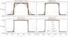Fig. 1.

DUSTYADVECT tests using the function f₁ (Eq. (30)). Dust density after one on period various grids (ℓ = 7 in blue, ℓ = 9 in orange, ℓ = 11 in green, ℓ = 13 in red) as a function of the position compared with the analytic solution (black solid line). We present this test using four different slope limiters. Top left: No predictor step. Top right: Minmod slope limiter. Bottom left: Van-Leer slope limiter. Bottom right: superbee slope limiter.

Another series of DUSTYADVECT tests are performed for different resolutions, using the Minmod slope limiter and without a predictor step. A smooth initial Gaussian-like function f₂ is imposed to quantify the truncation error in space of the scheme which writes, ∀x ∈ [0,L],

$\begin{matrix} f_{2} (x) = 0.01 + 0.1 exp [- {(\frac{x - L / 2}{L / 4})}^{2}] \cdot \end{matrix}$ $\begin{aligned} f_2\left(x\right) = 0.01 + 0.1 \exp \left[{-{\left(\frac{x-L/2}{L/4}\right)}^2}\right]\cdot \end{aligned}$ (31)

We use a very small timestep Δt = 10⁻⁸ to minimize the truncation errors in time compared with spatial errors. The results are compared at the same time t = 0.01 with the analytic solution using the L₂ norm

$\begin{matrix} L_{2} = \sqrt{\frac{\sum_{i = 1}^{N_{cell}} {| {ρ_{d}}_{RESULTS, i}^{n} - {ρ_{d}}_{ANALYTIC, i}^{n} |}^{2}}{N_{cell}}} \cdot \end{matrix}$ $\begin{aligned} L_{2}= \sqrt{\frac{\sum _{i=1}^{N_{\mathrm{cell} }}\left|{{\rho _{\mathrm{d} }}_{\mathrm{RESULTS} ,i}^n}-{{\rho _{\mathrm{d} }}_{\mathrm{ANALYTIC} ,i}^n}\right|^2}{N_{\mathrm{cell} }}}\cdot \end{aligned}$ (32)

Figure 2 shows the evolution of the L₂ norm with (blue squares) and without (orange diamonds) a prediction step as a function of the size of the cells for the Gaussian-like test. As expected, without prediction, the scheme has only a first-order accuracy in space, while it is a second-order scheme when the full predictor-corrector scheme with slope limiters are used.

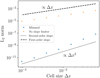Fig. 2.

DUSTYADVECT tests with an initial condition given by the function f₂ (Eq. (31)). L₂ (Eq. (32)) norm as a function of the cell size for the scheme using the Minmod slope limiter (blue squares) and without predictor step (orange diamonds). The results are compared with a first-order slope (dashed line) and a second-order slope (dotted line).

4.2. Dustydiffuse

When the hydrodynamical variables (pressure and dust ratio excluded) remain constant, Eq. (8) behaves as a non-linear diffusion equation. Pure dust diffusion tests can thus be performed. In the DUSTYDIFFUSE tests (Price & Laibe 2015), the hydrodynamical step is deactivated and t_s and c_s are set constant as well. Therefore, we only solve the following equation:

$\begin{matrix} \frac{\partial ρ_{d}}{\partial t} = \frac{\partial ρ_{d} w_{x}}{\partial x} \cdot \end{matrix}$ $\begin{aligned} \frac{\partial \rho _{\mathrm{d} }}{\partial t} = \frac{\partial \rho _{\mathrm{d} }{ w}_x}{\partial x}\cdot \end{aligned}$ (33)

An isothermal equation of state $P_{g} = c_{s}^{2} (1 - ϵ) ρ$ $P_{\mathrm{g}} =c_{\mathrm{s}}^2(1- \epsilon) \rho$ is considered. The advection velocity is then given by

$\begin{matrix} w_{x} = - t_{s} c_{s}^{2} \frac{\partial ϵ}{\partial x} ; \end{matrix}$ $\begin{aligned} { w}_x= -t_{\mathrm{s} } c_{\mathrm{s} }^2 \frac{\partial \epsilon }{\partial x}; \end{aligned}$ (34)

ρ being constant, the equation can be written as the a non-linear diffusion equation

$\begin{matrix} \frac{\partial ϵ}{\partial t} = t_{s} c_{s}^{2} \frac{\partial}{\partial x} (ϵ \frac{\partial ϵ}{\partial x}) \cdot \end{matrix}$ $\begin{aligned} \frac{\partial \epsilon }{\partial t} = t_{\mathrm{s} } c_{\mathrm{s} }^2 \frac{\partial }{\partial x} \left(\epsilon \frac{\partial \epsilon }{\partial x}\right)\cdot \end{aligned}$ (35)

Equation (35) has a self similar solution known as the Barenblatt-Pattle solution (Barenblatt 1952) that writes

$\begin{matrix} ϵ (t, x, C) = {(t_{s} c_{s}^{2} t)}^{- 1 / 3} (C - \frac{1}{6} \frac{x^{2}}{{(t_{s} c_{s}^{2} t)}^{2 / 3}}), \end{matrix}$ $\begin{aligned} \epsilon (t,x,C) = (t_{\mathrm{s} } c_{\mathrm{s} }^2 t)^{-1/3}\left(C- \frac{1}{6}\frac{x^2}{(t_{\mathrm{s} } c_{\mathrm{s} }^2 t)^{2/3}}\right), \end{aligned}$ (36)

where C is a constant depending on the initial conditions. We consider the following initial profile

$\begin{matrix} ϵ (t_{0}, x) = ϵ_{0} (1 - {(\frac{x}{x_{c}})}^{2}), \end{matrix}$ $\begin{aligned} \epsilon (t_0,x) = \epsilon _0 \left( 1 - \left(\frac{x}{x_{\mathrm{c} }}\right)^2\right) , \end{aligned}$ (37)

which is consistent with Eq. (36) if

$\begin{matrix} t_{0} = & \frac{C^{3}}{t_{s} c_{s}^{2} ϵ_{0}^{3}}, \\ C = & {(\frac{ϵ_{0} x_{c}}{\sqrt{6}})}^{2 / 3} \cdot \end{matrix}$ $\begin{aligned} t_0 =&\frac{C^3}{t_{\mathrm{s} } c_{\mathrm{s} }^2 \epsilon _0^3}, \nonumber \\ C =&\left(\frac{\epsilon _0 x_{\mathrm{c} }}{\sqrt{6}}\right)^{2/3}\cdot \end{aligned}$

We additionally set ρ = 1, t_s = 0.1, ϵ₀ = 0.1 and c_s = 1 and an AMR grid of ℓ_min = 4 and with ℓ_max = 10. The refinement criterion, based on the dust density gradient, forbids a variation of more than 5% between two cells.

Figure 3 shows a comparison between the outcome of the tests and the analytic solutions at t = 1, t = 5, t = 10 and t = 20. At each time the numerical results agree with the exact solution to a precision of less then 1% in L₂ norm. Even though our scheme is fundamentally designed for advection, it is also efficient at handling diffusion problems.

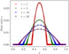Fig. 3.

DUSTYDIFFUSE tests. Dust ratio as a function of the position at t = 1 (red), t = 5 (green), t = 10 (blue), t = 20 (purple) compared with the exact solution (black solid lines).

4.3. Dustyshock

Another canonical test for gas and dust mixtures consists of 1D hydrodynamical shocks. For strongly coupled mixtures, these so-called DUSTYSHOCK tests are closely approximated by the same analytic solution as the usual Sod test (Sod 1978), but with the modified sound speed c̃_s

$\begin{matrix} {\tilde{c}}_{s} = c_{s} \sqrt{1 - ϵ_{0}}, \end{matrix}$ $\begin{aligned} \tilde{c}_{\mathrm{s} } ={c_{\mathrm{s} }} \sqrt{1- \epsilon _0}, \end{aligned}$

ϵ₀ being the initial dust ratio. The dust ratio ϵ remains almost constant through the shock; however, pressure bumps must occur where there is either a pressure or density gradient.

The same prescription as Laibe & Price (2014a) for the stopping time is used. It writes

$\begin{matrix} t_{s} = \frac{ϵ (1 - ϵ) ρ}{K}, \end{matrix}$ $\begin{aligned} t_{\mathrm{s} } = \frac{\epsilon (1- \epsilon ) \rho }{K}, \end{aligned}$

where K is the drag coefficient defined previously. This prescription is consistent with the expression of the stopping time presented before is convenient for tests since it allows us simply parametrize the coupling between the gas and dust phase.

A DUSTYSHOCK test is performed on an AMR grid with ℓ_min = 4 and ℓ_max = 13 with a high initial dust ratio. The grid is refined with a criterion that forbids dust density variations of more than 5% between two neighbor cells. Two distinct regions, representing the left and right half of the box, are set with different initial conditions given by

$\begin{matrix} {(ρ_{0}, v_{0}, {P_{g}}_{0}, ϵ_{0})}_{left} = (1, 0, 1, 0.5) \\ {(ρ_{0}, v_{0}, {P_{g}}_{0}, ϵ_{0})}_{right} = (0.125, 0, 0.1, 0.5) . \end{matrix}$ $\begin{aligned}&\left(\rho _0, \mathbf v _0, {P_{\mathrm{g} }}_0, \epsilon _0 \right)_{\mathrm{left} }= \left(1,0,1,{0.5}\right) \\&\left(\rho _0, \mathbf v _0, {P_{\mathrm{g} }}_0, \epsilon _0 \right)_{\mathrm{right} }= \left(0.125,0,0.1,{0.5}\right). \end{aligned}$

Finally, a drag coefficient K = 1000 and an adiabatic index γ = 1.4 are imposed.

Figure 4 shows the gas and dust densities, the velocity, and the gas pressure as a function of the position at t = 0.2. The Sod solution with the modified sound speed is very well recovered.

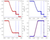Fig. 4.

DUSTYSHOCK with ϵ = 0.5. Top left: gas density as a function of position. Top right: same but for dust. Bottom left: gas pressure. Bottom right: gas and dust velocities. The AMR level (right axis) is represented with dotted blue lines. The analytic solution is given by the black solid lines. Red circles and blue crosses indicate gas and dust numerical quantities, respectively.

4.4. Dustywave

The 1D DUSTYWAVE test (Laibe & Price 2011) consists in following the evolution of an isothermal sound wave in a gas and dust mixture. Small periodic perturbations on the Eqs. (6) on the density, the dust ratio, the pressure, and the velocity are imposed

$\begin{matrix} ρ = ρ_{0} + δ ρ_{0}, \\ ϵ = ϵ_{0} + δ ϵ_{0}, \\ P_{g} = {P_{g}}_{0} + δ {P_{g}}_{0}, \\ ν_{x} = 0 + δ {ν_{x}}_{0}, \end{matrix}$ $\begin{aligned}&\rho = \rho _0+ \delta \rho _0, \nonumber \\&\epsilon = \epsilon _0 + \delta \epsilon _0, \nonumber \\&{P_{\mathrm{g} }}= {P_{\mathrm{g} }}_0 + \delta {P_{\mathrm{g} }}_0, \nonumber \\&{\nu _x} = 0 +\delta {\nu _x}_0, \end{aligned}$

where the index 0 and the symbol δ indicate respectively the initial uniform quantities and the perturbations. Laibe & Price (2011) provide the analytic solution for this test. They find that the sound waves propagate with the modified sound speed c̃_s and are damped because of the dust inertia. Large grains damp these sound waves faster than small grains as they are more massive.

Three DUSTYWAVE tests are performed using different drag coefficients K = 50 (K50, strong back-reaction regime), K = 100 (K100) and K = 1000 (K1000,weak back-reaction regime). The initial perturbations are in the form

$\begin{matrix} δ ρ_{0} = ρ_{0} δ sin (2 π \frac{x}{L}), \\ δ {ν_{x}}_{0} = ν_{0} δ sin (2 π \frac{x}{L}), \\ δ {P_{g}}_{0} = (1 - ϵ_{0}) c_{s, 0}^{2} δ ρ_{0}, \\ δ ϵ_{0} = 0, \end{matrix}$ $\begin{aligned}&\delta \rho _0 = \rho _0 \delta \sin \left(2 \pi \frac{x}{L}\right), \nonumber \\&\delta {\nu _x}_0 = \nu _0 \delta \sin \left(2 \pi \frac{x}{L}\right),\nonumber \\&\delta {P_{\mathrm{g} }}_0 = \left(1-\epsilon _0\right) c_{\mathrm{s} ,0}^2 \delta \rho _0,\nonumber \\&\delta \epsilon _0 = 0, \end{aligned}$

where x is the position in the box, L is the box length, c_s, 0 is the initial sound speed, and δ is a parameter that sets the amplitude of the perturbation. The initial uniform state is set such as that

$\begin{matrix} ρ_{0} = 2, \\ ϵ_{0} = 0.5, \\ ν_{0} = 1, \\ c_{s, 0} = 1 . \end{matrix}$ $\begin{aligned}&\rho _0 = 2, \\&\epsilon _0 = 0.5, \\&\nu _0 = 1, \\&c_{\mathrm{s} ,0} = 1. \end{aligned}$

The adiabatic index of the gas is γ = 1.000001² to simulate an isothermal soundwave propagation. The initial perturbation has a relative amplitude δ = 10⁻⁴. The simulation box has a size L = 1.0 and the grid is taken as uniform with 64 cells. The timestep Δt = 10⁻⁴ is the same for the three tests and respects the stability condition for the considered drag coefficients.

Figures 5 and 6 show the velocity ν_x and the perturbation density δρ = ρ − ρ₀ for both gas and dust at t = 4.5 for these three tests. The amplitude of the damping increases with a decreasing K and the results are increasingly less accurate as the errors due to the diffusion approximation increase, consistently with the theory (Laibe & Price 2011; Price & Laibe 2015). Larger grains, i.e, with smaller K, have more inertia and allow an efficient damping of the gas.

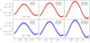Fig. 5.

DUSTYWAVE test. Velocity of the gas (top) and dust (bottom) phase as a function of the position at t = 4.5 for the K50, K100 and K1000 tests (from left to right) compared with the analytical solution (black lines) given by Laibe & Price (2011).

Fig. 6.

DUSTYWAVE test. Same as in Fig. 5 but for the density perturbations.

We perform DUSTYWAVE tests on uniform grids with resolutions ranging from ℓ = 5 to ℓ = 9, with a small timestep Δt = 10⁻⁵ and for K = 50. We also perform runs on AMR grids with coarse resolutions ranging from ℓ_min = 4 to ℓ_min = 8. For these tests, the cells for x ∈ [0.25,0.75] have a level of refinement ℓ_max = ℓ_min + 1. We test the order of our scheme and measure the accuracy of numerical solution against a solution of reference obtained at very high resolution (ℓ = 11) in both time and space (Δt = 10⁻⁶). We do not compare the results with the analytic solution presented above as it not exact in the diffusion approximation. Figure 7 shows the L₂ errors obtained when increasing the number of cells. The scheme is first-order in space without correction and second-order when using the Minmod limiter. In the presence of AMR, the scheme keeps a second-order accuracy in space for low resolution but deteriorates at high resolutions. This is due to the estimate of the pressure gradient that is first-order at a refined interface. At high resolution, the error is smaller (almost two orders of magnitude) than the tests without a predictor step.

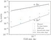Fig. 7.

DUSTYWAVE numerical convergence tests. L₂ norm as a function of the minimum cell size for the scheme using the Minmod slope limiter (blue squares), without predictor step (orange diamonds) and with AMR (green circles). The results are compared with a first-order slope (dashed line) and a second-order slope (dotted line).

4.5. Disk settling

The SETTLING test, introduced by Price & Laibe (2015), is designed to test the algorithm in realistic astrophysical conditions. It simulates the local settling of dust grains in a disk in hydrostatic equilibrium. As in Price & Laibe (2015), we set an analytic gravitational force

$\begin{matrix} f_{grav} = - \frac{G M_{⋆} y}{{(y^{2} + r^{2})}^{3 / 2}}, \end{matrix}$ $\begin{aligned} f_{\mathrm{grav} }= - \frac{ \mathcal{G} M_{\star } { y} }{{({ y}^2+r^2)}^{3/2}}, \end{aligned}$

where 𝒢 is the gravitational constant, M_⋆ is the mass of the central star, y is the altitude and r the cylindrical radius at which the disk is simulated. The gas density at hydrostatic equilibrium for |y|≪r is

$\begin{matrix} ρ_{g} = ρ_{g, 0} e^{- \frac{y^{2}}{2 H^{2}}}, \end{matrix}$ $\begin{aligned} \rho _{\mathrm{g} } = \rho _{\mathrm{g} ,0} \mathrm{e}^{-\frac{{ y}^2}{2 \mathcal{H} ^2}}, \end{aligned}$

where ℋ is the local scale height of the disk, which is determined by the ratio ℋ/r = 0.05. We then assume an isothermal equation of state where the imposed soundspeed c_s is

$\begin{matrix} c_{s} = H Ω_{k}, \end{matrix}$ $\begin{aligned} c_{\mathrm{s} } = \mathcal{H} \Omega _{\mathrm{k} }, \end{aligned}$ (38)

Ω_k being the Keplerian angular velocity at the radius r. Finally, a uniform initial dust ratio ϵ₀ is imposed.

In the terminal velocity approximation, the analytic solution for the dust velocity is directly set by the pressure gradient that compensates the gravitational force, hence

$\begin{matrix} ν_{d, y} = w_{Y} = - St Ω_{k} \frac{y}{{(1 + {(y / r)}^{2})}^{3 / 2}}, \end{matrix}$ $\begin{aligned} \nu _{\mathrm{d} ,{ y}}= { w}_Y = - \mathrm{St} \Omega _{\mathrm{k} } \frac{{ y}}{(1+({ y}/r)^2)^{3/2}}, \end{aligned}$ (39)

which is the limit at low Stokes number (St = Ω_kt_s in this case) of the expression given by Hutchison et al. (2018). As the gas approximately remains in equilibrium, solving the settling problem consists in solving

$\begin{matrix} \frac{\partial ρ_{d}}{\partial t} + \frac{\partial ρ_{d} w_{y}}{\partial y} = 0 . \end{matrix}$ $\begin{aligned} \frac{\partial \rho _{\mathrm{d} } }{\partial t}+\frac{\partial \rho _{\mathrm{d} } { w}_{ y} }{\partial { y}} = 0. \end{aligned}$ (40)

Even though the density can, in principle, be determined using the same method as the velocity, it relies on the hypothesis of an infinite dust reservoir that is inconsistent with our choice of boundaries. We choose to compare our results with a numerical solution as in Hutchison et al. (2018). We use a similar Crank-Nicholson scheme to get this solution, except that it only solves the dust density equation using the analytic dust velocity.

We perform a 2D SETTLING test at a disk orbiting around a solar mass star at radius of 50 au. The simulation box has periodic boundary conditions and L = 20 au, which is approximately 8ℋ. As in Price & Laibe (2015) and Hutchison et al. (2018), the initial mid-plane gas density ρ_g ≈ 6 × 10⁻¹³ g cm⁻³. We also set an initial dust ratio of 4.99 × 10⁻³ of millimeter grains with an intrinsic density of ρ_grain = 3 g cm⁻³. The adiabatic index of the gas is γ = 5/3.

A first test with a uniform grid at level ℓ = 8 is performed. Figure 8 shows the dust ratio as a function of y. As can be seen, the results are essentially similar to those obtained in Price & Laibe (2015) and Hutchison et al. (2018).

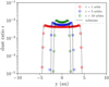Fig. 8.

SETTLING test on a uniform grid at level ℓ = 8 with millimeter-size dust grains. Dust ratio at t = 1 (red circles), 5 (blue circles), and 10 orbits (green circles) as a function of the altitude.

4.6. Multigrain

4.6.1. Example 1: Dustydiffuse

To benchmark the implementation of the multiple dust species in the code, ten DUSTYDIFFUSE tests are performed on uniform grids of ℓ = 7. They are operated with one dust phase and with this same phase split with 𝒩 ∈ [2,10] (MULTIGRAIN). All the dust bins have the same intrinsic properties. As all the tests are equivalent, it is expected that they give the same results. The parameters used are the same as in Sect. 4.2.

Figure 9 shows the total dust density as a function of position with 𝒩 = 5 (top) and 𝒩 = 1 (bottom) at t = 1, t = 5, t = 10, and t = 20. The results agree for the MULTIGRAIN simulation and for the single phase simulation to machine precision.

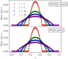Fig. 9.

Comparison between multiple phase with 𝒩 = 5 (top) and an equivalent single phase (bottom) DUSTYDIFFUSE test. Dust ratio as a function of the position at t = 1 (red), t = 5 (green), t = 10 (blue) and t = 20 s (purple) compared with the exact solution (black solid lines).

Figure 10 shows the CPU time as a function of the number of species 𝒩. We see that the MULTIGRAIN simulations are not very expensive. The CPU time agrees more with a square root scaling with 𝒩 than a linear one. As discussed by Hutchison et al. (2018) with the MULTIGRAIN algorithm in the PHANTOM code (Price et al. 2017), the monofluid formalism is a highly computationally effective tool to treat multiple phases.

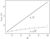Fig. 10.

CPU time t_CPU of the ten equivalent DUSTYDIFFUSE tests as a function of the number of species 𝒩.

4.6.2. Example 2: Dustywave

In this section, we test the cumulative back-reaction of dust on the gas and the interaction between dust species. To benchmark our MULTIGRAIN implementation in a strong back-reaction regime we run a DUSTYWAVE simulation with two dust species. The initial barycentric velocity is a sinusoidal perturbation of amplitude 10⁻⁴, the other variables are not initially perturbed. We numerically integrate the linearly perturbed equations of gas and dust mixtures assuming solutions of the type A(t)exp(ikx) as in Laibe & Price (2014c) to obtain our reference solution. The test is performed with a uniform grid of ℓ = 9 and timesteps given by the CFL condition. In this test, we consider two dust phases and a total initial dust ratio of 0.5. The first bin has a drag coefficient K = 50 and an initial dust ratio of 0.4, the second has a drag coefficient K = 1000 and an initial dust ratio of 0.1. In this case, we expect the first dust species to damp the gas efficiently.

Figure 11 shows the amplitude of the density perturbations (gas and dust) and velocity (gas) compared with the reference solution. Our results are in excellent agreement with the reference solution in terms of amplitude, period and damping rate. As expected the damping of the gas is significant. This emphasizes the fundamental role of the cumulative back-reaction on the dynamics of dust grains in presence of multiple species as the second phase K = 1000 could not damp the gas as efficiently (see Sect. 4.4).

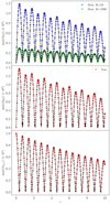Fig. 11.

MULTIGRAIN DUSTYWAVE test. The three panels show the evolution of the maximum amplitude of the perturbation for the dust densities (top), the gas density (middle), and the gas velocity (bottom). The K = 50 and K = 1000 dust phases are shown with blue and green circles respectively. The red circles represent the gas. The semi-analytic solution is given by the dashed black line.

4.6.3. Example 3: Disk settling

The disk SETTLING test presented in Sect. 4.5 is nicely adapted to test our MULTIGRAIN solver in realistic conditions. Dust grains of various sizes are present in protoplanetary disks and they experience different dynamical evolutions. To test the solver in these conditions, a settling test with ten dust species is performed with a resolution of ℓ = 8. As before, the intrinsic grain density is 3 g cm⁻³, but every species is characterized by a proper dust ratio ϵ_j and grain size s_grain, j. These quantities are determined using a MRN-like distribution³, we use the same values for the minimum and maximum grain size as in Hutchison et al. (2018). The details of the size distribution are summarized in Table 1, which also shows the stopping time of each species in the mid-plane of the disk.

Table 1.

Dust distribution and stopping time at z = 0 for the MULTIGRAIN SETTLING test.

Figure 12 shows the dust ratio and velocity of every species after ten orbits compared with the one-species solution, which is a good approximation as long as the cumulative back-reaction on the gas is small. Again, the solution is very well captured by our solver.

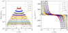Fig. 12.

MULTIGRAIN SETTLING test. Dust ratios and dust velocities (circles) of the ten phases of the SETTLING test after ten orbits compared with the numerical (dotted black lines) and analytic (black lines) one-species solution.

Figure 13 shows the dust densities in the (xy)-plane. There is no dispersion of the values in the x-direction, and the initial symmetry of the problem is conserved to machine precision which originate from the Eulerian nature of the numerical scheme. As in previous studies, we see that ten orbits are enough to efficiently separate the dust phases. We note that an orbit at 50 au is approximately 353 years which is a few hundred times smaller than the free-fall timescale of a typical protostellar cloud of density ≈10⁻¹⁹ g cm⁻³ (Andre et al. 2000) which is approximately 10⁵−10⁶ years. An efficient settling is thus expected to happen during the collapse of this cloud, especially for large grains, e.g., s_grain > 10⁻² cm here, for which the typical settling timescale is a few orbits.

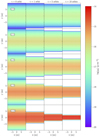Fig. 13.

MULTIGRAIN SETTLING test. Dust density for the species j = 2, 4, 6, 8, and 10 in the (xy)-plane at t = 0, 1, 5, and 10 orbits.

As in Hutchison et al. (2018), we are interested in the effects of the interaction between different dust species. Figure 14 shows a zoom of the vertical profile of ϵ₁ as a function of y. The behavior of this phase is similar to what was observed in Hutchison et al. (2018). The dashed black line shows the one-species solution. As we see, for this species, the discrepancies between the one-species solution and the MULTIGRAIN test are on the order of magnitude of the variations of ϵ₁ at the dust front, which emphasizes the fundamental character equivalent stopping time in MULTIGRAIN simulations.

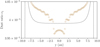Fig. 14.

MULTIGRAIN SETTLING test. Magnification of the dust front as a function of y for the j = 1 dust species (brown circles) compared with the one-species solution (dotted line). These dust grains are dragged by the gas, which is itself submitted to the cumulative back-reaction of all the other dust species through the gas, hence the difference is the one-species solution.

5. Dusty protostellar collapses

The final test of the algorithm verifies again that both gas and dust are sensitive to gravity and the 3D implementation of the solver.

5.1. Dustycollapse

To study the collapse of a dense core, 3D canonical test cases, introduced by Boss & Bodenheimer (1979), but in the presence of dust (DUSTYCOLLAPSE) are performed to follow dust dynamics during the formation of the first Larson core (Larson 1969). The initial dense core, composed with gas and dust, has a mass M₀, a uniform density ρ₀ and a dust ratio ϵ₀. Its radius R₀ is set by the ratio between the thermal and gravitational energies α

$\begin{matrix} α = \frac{5}{2} \frac{(1 - ϵ_{0}) R_{0}}{G M_{0}} \frac{k_{B} T_{g}}{μ m_{H}}, \end{matrix}$ $\begin{aligned} \alpha = \frac{5}{2}\frac{(1-\epsilon _0) R_0 }{ \mathcal{G} M_0}\frac{k_{\mathrm{B} }T_{\mathrm{g} }}{\mu m_{\mathrm{H} }}, \end{aligned}$ (41)

where k_B is the Boltzmann constant, μ is the mean molecular weight, m_H the hydrogen atomic mass, and T_g the initial gas temperature.

A barotropic equation of state is used to describe the optically thick regime at which the evolution is adiabatic. It writes

$\begin{matrix} \frac{P_{g}}{(1 - ϵ) ρ} = c_{s}^{2} [1 + {((1 - ϵ) \frac{ρ}{ρ_{ad}})}^{γ - 1}], \end{matrix}$ $\begin{aligned} \frac{P_{\mathrm{g} }}{(1-\epsilon )\rho } = c_{\mathrm{s} }^2 \left[1+ \left((1-\epsilon )\frac{\rho }{\rho _{\mathrm{ad} }} \right)^{\gamma -1}\right], \end{aligned}$ (42)

the evolution becoming adiabatic above the critical density ρ_ad = 10⁻¹³ g cm⁻³ (Larson 1969). For the sake of simplicity, this critical density is taken constant in this paper. A dependency with the dust ratio will be discussed in future works.

As in Tricco et al. (2017), we consider an unique grain density ρ_grain = 3 g cm⁻³ which is a good approximation for a combination of carbonaceous and silicate grains.

5.2. Setup

All the models are set with M₀ = 1 M_⊙, μ = 2.31, γ = 5/3, and T_g = 10 K. AMR grids of ℓ_min = 5 and ℓ_max = 17 are considered. With respect to the criterion given by Truelove et al. (1997) to avoid artificial clumps, the grid is refined to impose at least 15 points per Jeans length. The region surrounding the core has a density that is one hundred time lower than the initial core but the same temperature.

The initial density and pressure gradients between the core and the ambient medium are numerical artifacts. To avoid unphysical variations of the dust ratio in these regions and unnecessary constraints on the timestep, the differential advection velocity w_k is set to zero outside the initial core.

We consider the first hydrostatic core as the region where the gas density is higher than 10^−12.5 g cm⁻³.

5.3. Validity of the diffusion approximation

The diffusion approximation is valid as long as the stopping time t_s is shorter than the dynamical timescale which is, for gravitational collapses, roughly the free-fall time

$\begin{matrix} t_{ff} \equiv \sqrt{\frac{3 π}{32 G ρ}} \cdot \end{matrix}$ $\begin{aligned} t_{\mathrm{ff} } \equiv \sqrt{\frac{3 \pi }{32 \mathcal{G} \rho }}\cdot \end{aligned}$

With an initial dust ratio of 0.01 and a temperature of 10 K, the Stokes number is

$\begin{matrix} St \sim 0.114 (\frac{M_{0}}{1 M_{⊙}}) (\frac{ρ_{grain}}{3 g {cm}^{- 3}}) (\frac{s_{grain}}{0.05 cm}) {(\frac{α}{0.5})}^{3 / 2} < 1 . \end{matrix}$ $\begin{aligned} \mathrm{St} \sim 0.114\left(\frac{M_0}{1\,M_{\odot }}\right) \left(\frac{\rho _{\mathrm{grain} }}{3\,\mathrm{g} \,\mathrm{cm} ^{-3}}\right) \left(\frac{s_{\mathrm{grain} }}{0.05\, \mathrm{cm} } \right) \left({\frac{\alpha }{0.5}}\right)^{3/2} < 1. \end{aligned}$ (43)

For a wide range of density and grain size the stopping time is short compared to the dynamical timescale. Initially, the stopping time is shorter than the free-fall timescale for grain sizes up to ≃4 mm. However, as the Stokes number may vary, the validity of the approximation needs to be discussed during the collapse (see Sect. 5.5).

5.4. Free-fall timescale for strongly coupled mixtures

A core only composed with gas would collapse at the following free-fall timescale

$\begin{matrix} t_{ff, g} \equiv \sqrt{\frac{3 π}{32 G ρ_{g}}} \cdot \end{matrix}$ $\begin{aligned} t_{\mathrm{ff,g} } \equiv \sqrt{\frac{3 \pi }{32 \mathcal{G} \rho _{\mathrm{g} }}}\cdot \end{aligned}$

For a perfectly coupled gas and dust mixture (t_s ≪ t_ff) it writes

$\begin{matrix} t_{ff} = \sqrt{\frac{3 π}{32 G ρ}} \cdot \end{matrix}$ $\begin{aligned} t_{\mathrm{ff} } = \sqrt{\frac{3 \pi }{32 \mathcal{G} \rho }}\cdot \end{aligned}$

In the context of the Boss and Bodenheimer test, this timescale indirectly depends on the initial dust ratio

$\begin{matrix} t_{ff} = \frac{π}{5 \sqrt{5}} G M_{0} {(\frac{α μ m_{H}}{k_{b} T_{g} (1 - ϵ_{0})})}^{3 / 2} \cdot \end{matrix}$ $\begin{aligned} t_{\mathrm{ff} } = \frac{\pi }{5\sqrt{5}}\mathcal{G} M_{0} \left( \frac{\alpha \mu m_{\mathrm{H} }}{k_{\mathrm{b} }T_{\mathrm{g} } (1-\epsilon _0)}\right)^{3/2}\cdot \end{aligned}$ (44)

Physically, this is due to the fact that two cores with the same initial α but different ϵ₀ have different initial radius, hence free-fall timescale. Indeed, R₀ increases with ϵ₀ so that the gas provides the same thermal support against gravity.

To test this relation, non-rotating DUSTYCOLLAPSE with various dust ratios and the same α = 0.5 are performed. The condition t_s ≪ t_ff is ensured by considering very small grains with s = 10⁻⁷ cm. Figure 15 shows the ratio of the free-fall timescale of a dusty cloud to that of a pure-gas cloud compared with the analytical solution. We define the free-fall timescale as the time at which the peak density reaches ρ_ad. The scaling relation is very well verified. As expected, the gas, and the dust, are sensitive to gravity and fall at the mixture free-fall timescale.

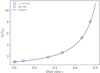Fig. 15.

Ratio of the free-fall timescale of the mixture to the free-fall timescale of the gas. The red circle corresponds to the fiducial simulation with gas only, and the blue circles correspond to gas and dust mixtures for various dust ratios. The black solid line is the analytical solution.

5.5. Core properties

Non-rotating DUSTYCOLLAPSE of α = 0.5 are performed with an initial dust-to-gas ratio of 1% (corresponding to ϵ ∼ 0.00990099). Single grain species of size 1 μm (Col1), 10 μm (Col10) and 100 μm (Col100) are considered. The results are compared, when the gas maximum density reaches 10⁻¹¹ g cm⁻³, with a fiducial collapse without any treatment of dust (ColGAS).

Figure 16 shows the total mass of the first hydrostatic core M_core, the dust mass ratio M_d/M_core and its formation time t_core as a function of the grain size (bottom x-axis) and the initial Stokes number (top x-axis). The first core properties depend on the amount of dust in the initial dense core. In the fiducial ColGAS test, the gas density is assimilated to the total density, as is often the case in the literature. This results in a lower first-core mass and a shorter formation time. We note that the barotropic equation of state implicitly assumes a constant dust-to-gas ratio of 1%, which is slightly inconsistent. Dust-to-gas ratios might be even higher in core forming regions (Hopkins & Lee 2016; Tricco et al. 2017) which could lead to even more important discrepancies. In terms of dynamics, small grains (s < 100 μm) do not have a significant impact as they fall alongside the gas. However, the differential velocity between the gas and the dust is proportional to the stopping time, hence large grains (s ≥ 100 μm) tend to fall substantially faster than the gas. Their infall provokes a slight acceleration of the first core formation as it changes the balance between the gravity and the thermal support of the gas. The mass of the core decreases as the grain size increases because the gas has less time to be accreted during the collapse. The settling of dust in the central regions of the core, however, leads to an increase in M_d/M_core.

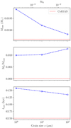Fig. 16.

Properties of the first Larson core when ρ_g ∼ 10⁻¹¹ g cm⁻³ for Col1, Col10, and Col100. The core mass, the dust mass ratio, and the formation time are shown as a function of the grain size (blue circles). The results are compared with the fiducial ColGAS simulation (dashed red lines). The top x-axis shows the initial Stokes number in the core St₀.

Figures 17 and 18 show the radial profiles for the Col10 and Col100 tests, respectively, of the gas density, the dust ratio, the gas and dust velocities, and the Stokes number. As can be seen, the strong dust depletion in the outer regions of the collapse provides the enrichment of the core. However, as the damping is more efficient in the high density regions (see the velocities v_g ≈ v_d), the dust ratio increases at a slower rate in the inner regions of the collapse, i.e, the first core. If the maximum increase of dust ratio in the outer regions of the collapse is about ∼20% for the Col10 test, it goes up to ∼300% for the Col100 test. We see in the Col100 case that the terminal velocity approximation probably leads to non-negligible errors as the Stokes number is close to one in the outer regions of the collapse . More accurate simulations using a future implementation of the full monofluid formalism (Laibe & Price 2014a) should investigate these errors.

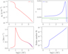Fig. 17.

Radial profiles of the Col10 test. Top left: gas density. Top right: dust ratio. Bottom left: gas and dust velocities. Bottom right: stokes number. The horizontal green line corresponds to a dust-to-gas ratio of 1%.

Fig. 18.

Same as Fig.17, but for the Col100 test.

If initial solid-body rotation is considered, it is expected that the large dust grains will settle in the mid-plane of the protoplanetary disk (Bate & Lorén-Aguilar 2017). Future works will take this into account and the presence of multiple grain species as well.

6. Conclusions and perspectives

We have presented an Eulerian approach to treat the dynamics of small dust grains. It is efficient in the diffusion regime and can be employed to treat multiple dust species simultaneously and efficiently. After a summary of the theory, we presented the numerical scheme that we implemented in the AMR code RAMSES. It successfully passed the canonical validation tests for advection schemes and dust dynamics solvers, i.e, DUSTYADVECT, DUSTYDIFFUSE, DUSTYSHOCK, DUSTYWAVE, SETTLING, and DUSTYCOLLAPSE. We show that our scheme has a second-order accuracy in space on uniform grids and intermediate between first- and second-order on AMR grids. The method also appears to efficiently treat a non-linear diffusion problem. The DUSTYSHOCK, DUSTYWAVE, SETTLING and DUSTYCOLLAPSE, show that the waves and shock propagate at the correct velocity, and that the dust phase feels the common forces between gas and dust, e.g., gravity. The DUSTYDIFFUSE test operated with a split dust phase shows that our method is able to efficiently treat multiple dust species simultaneously as the computation time scales in $\sqrt{N}$ ${\sqrt{N}}$ . We emphasize the importance of the cumulative back-reaction on both the gas and the dust with the MULTIGRAIN DUSTYWAVE tests. We show with a MULTIGRAIN SETTLING test that our solver efficiently treats multiple phases in a realistic astrophyiscal environment. We also observe the same interactions between the dust phases that were uncovered in Hutchison et al. (2018).

The method is applied to study dust dynamics during the formation of the first hydrostatic core. As found in Bate & Lorén-Aguilar (2017), grains larger than s ≃ 100 μm can fall substantially faster than the gas. Above this size, the grains settle in the core, enriching its dust content and speeding up the collapse. We showed that the core properties are not affected very much by the dynamics of dust for small grains (s < 100 μm). However, they depend on the presence of dust itself as the thermal-to-gravitational energy ratio α depends on both the gas and the dust density.

The scheme was presented, for simplicity, in the hydrodynamical case; however, it is implemented in the radiation non-ideal MHD version of RAMSES. Realistic simulations of star formation would require us to consider the impact of dust on magnetic fields and radiative transfer coupling with the mixture. In that perspective, later work will focus on taking into account the impact of the variation of the dust ratio on the opacity and the magnetic resistivities.

In the paper II we will discuss in more detail the grain dynamics during the collapse of rotating clouds with MULTIGRAIN simulations.

¹

||.|| indicates the L2 norm of either a tensor or a vector.

²

Taking exactly γ = 1 is not possible with RAMSES as the internal energy is computed as $\frac{P_{g}}{γ - 1}$ $\frac{P_{\mathrm{g}}}{\gamma -1}$ .

³

$ϵ (s_{grain}) \propto s_{grain}^{4 - m}$ $\epsilon \left(s_{\mathrm{grain}}\right) \propto s_{\mathrm{grain}}^{4-m}$ with m = 3.5.

Acknowledgments

First, we sincerely thank the referee for providing extremely useful remarks and ideas which helped to significantly improve the quality of our work. We acknowledge financial support from the Programme National de Physique Stellaire (PNPS) of CNRS/INSU, CEA, and CNES, France. This work was granted access to the HPC resources of CINES (Occigen) under the allocation DARI A0020407247 made by GENCI. Computations were also performed at the Common Computing Facility (CCF) of the LABEX Lyon Institute of Origins (ANR-10-LABX-0066). This work took part under the programs ISM3D and Core2disk of the PSI2 project funded by the IDEX Paris-Saclay, ANR-11-IDEX-0003-02. This project was partly supported by the IDEXLyon project (contract nANR-16-IDEX-0005) under the auspices University of Lyon. Some of the DUSTYCOLLAPSE plots were generated using the very efficient Osiris library developed by Neil Vaytet, Tommaso Grassi and Matthias González whom we thank. In particular, we thank Matthias González again for his useful advice on the paper. We also thank Daniel Price for his useful advice and Mark Hutchison for providing his solver to get the solution of the settling test. This project has received funding from the European Union’s Horizon 2020 research and innovation program under the Marie Skłodowska-Curie grant agreement No 823823.

References

Andre, P., Ward-Thompson, D., & Barsony, M. 2000, Protostars and Planets IV, 59 [Google Scholar]
Ayliffe, B. A., Laibe, G., Price, D. J., & Bate, M. R. 2012, MNRAS, 423, 1450 [NASA ADS] [CrossRef] [Google Scholar]
Barenblatt, G. 1952, Prikladnaya Matematika i Mekhanika, 16, 679 [Google Scholar]
Bate, M. R., & Lorén-Aguilar, P. 2017, MNRAS, 465, 1089 [NASA ADS] [CrossRef] [Google Scholar]
Berger, M. J., & Oliger, J. 1984, J. Comput. Phys., 53, 484 [NASA ADS] [CrossRef] [MathSciNet] [Google Scholar]
Boss, A. P., & Bodenheimer, P. 1979, ApJ, 234, 289 [NASA ADS] [CrossRef] [Google Scholar]
Chen, J.-W., & Lin, M.-K. 2018, MNRAS, 478, 2737 [NASA ADS] [CrossRef] [Google Scholar]
Chiang, E. 2008, ApJ, 675, 1549 [CrossRef] [Google Scholar]
Commerçon, B., Hennebelle, P., Audit, E., Chabrier, G., & Teyssier, R. 2008, A&A, 482, 371 [NASA ADS] [CrossRef] [EDP Sciences] [Google Scholar]
Commerçon, B., Teyssier, R., Audit, E., Hennebelle, P., & Chabrier, G. 2011, A&A, 529, A35 [NASA ADS] [CrossRef] [EDP Sciences] [Google Scholar]
Commerçon, B., Debout, V., & Teyssier, R. 2014, A&A, 563, A11 [NASA ADS] [CrossRef] [EDP Sciences] [Google Scholar]
Compiègne, M., Verstraete, L., Jones, A., et al. 2011, A&A, 525, A103 [NASA ADS] [CrossRef] [EDP Sciences] [Google Scholar]
Courant, R., Friedrichs, K., & Lewy, H. 1928, Mathematische Annalen, 100, 32 [Google Scholar]
Courant, R., Isaacson, E., & Rees, M. 1952, Commun. Pure Appl. Math., 5, 243 [CrossRef] [Google Scholar]
Dubois, Y., & Commerçon, B. 2016, A&A, 585, A138 [NASA ADS] [CrossRef] [EDP Sciences] [Google Scholar]
Epstein, P. S. 1924, Phys. Rev., 23, 710 [NASA ADS] [CrossRef] [Google Scholar]
Fromang, S., Hennebelle, P., & Teyssier, R. 2006, A&A, 457, 371 [NASA ADS] [CrossRef] [EDP Sciences] [Google Scholar]
Gingold, R. A., & Monaghan, J. J. 1977, MNRAS, 181, 375 [Google Scholar]
Godunov, S. K. 1959, Mat. Sb. (N.S.), 47, 271 [Google Scholar]
González, M., Vaytet, N., Commerçon, B., & Masson, J. 2015, A&A, 578, A12 [NASA ADS] [CrossRef] [EDP Sciences] [Google Scholar]
Harsono, D., Bjerkeli, P., & van der Wiel, M. H. D. 2018, Nat. Astron., 2, 646 [NASA ADS] [CrossRef] [Google Scholar]
Harten, A. 1983, J. Comput. Phys., 49, 357 [NASA ADS] [CrossRef] [MathSciNet] [Google Scholar]
Harten, A., Lax, D. P., & van Leer, B. 1983, SIAM Rev., 25, 35 [Google Scholar]
Hennebelle, P. 2018, A&A, 611, A24 [NASA ADS] [CrossRef] [EDP Sciences] [Google Scholar]
Hopkins, P. F., & Lee, H. 2016, MNRAS, 456, 4174 [NASA ADS] [CrossRef] [Google Scholar]
Hutchison, M., Price, D. J., & Laibe, G. 2018, MNRAS, 476, 2186 [NASA ADS] [CrossRef] [Google Scholar]
Laibe, G., & Price, D. J. 2011, MNRAS, 418, 1491 [NASA ADS] [CrossRef] [Google Scholar]
Laibe, G., & Price, D. J. 2012, MNRAS, 420, 2365 [NASA ADS] [CrossRef] [Google Scholar]
Laibe, G., & Price, D. J. 2014a, MNRAS, 440, 2136 [NASA ADS] [CrossRef] [Google Scholar]
Laibe, G., & Price, D. J. 2014b, MNRAS, 440, 2147 [NASA ADS] [CrossRef] [Google Scholar]
Laibe, G., & Price, D. J. 2014c, MNRAS, 444, 1940 [NASA ADS] [CrossRef] [Google Scholar]
Larson, R. B. 1969, MNRAS, 145, 271 [NASA ADS] [CrossRef] [Google Scholar]
Lax, P., & Wendroff, B. 1960, Commun. Pure Appl. Math., 13, 217 [CrossRef] [Google Scholar]
Lin, M.-K., & Youdin, A. N. 2017, ApJ, 849, 129 [NASA ADS] [CrossRef] [Google Scholar]
Lorén-Aguilar, P., & Bate, M. R. 2014, MNRAS, 443, 927 [NASA ADS] [CrossRef] [Google Scholar]
Lorén-Aguilar, P., & Bate, M. R. 2015, MNRAS, 454, 4114 [NASA ADS] [CrossRef] [Google Scholar]
Lucy, L. B. 1977, AJ, 82, 1013 [NASA ADS] [CrossRef] [Google Scholar]
Marchand, P., Masson, J., Chabrier, G., et al. 2016, A&A, 592, A18 [NASA ADS] [CrossRef] [EDP Sciences] [Google Scholar]
Marchand, P., Commercon, B., & Chabrier, G. 2018, A&A, 619, A37 [NASA ADS] [CrossRef] [EDP Sciences] [Google Scholar]
Mathis, J. S., Rumpl, W., & Nordsieck, K. H. 1977, ApJ, 217, 425 [NASA ADS] [CrossRef] [Google Scholar]
Masson, J., Teyssier, R., Mulet-Marquis, C., Hennebelle, P., & Chabrier, G. 2012, ApJS, 201, 24 [NASA ADS] [CrossRef] [Google Scholar]
Pagani, L., Steinacker, J., Bacmann, A., Stutz, A., & Henning, T. 2010, Science, 329, 1622 [NASA ADS] [CrossRef] [PubMed] [Google Scholar]
Price, D. J., & Laibe, G. 2015, MNRAS, 454, 2320 [NASA ADS] [CrossRef] [Google Scholar]
Price, D. J., Wurster, J., & Nixon, C. 2017, Astrophysics Source Code Library [record ascl:1709.002] [Google Scholar]
Roe, P. L. 1986, Annu. Rev. Fluid Mech., 18, 337 [Google Scholar]
Rosdahl, J., & Teyssier, R. 2015, MNRAS, 449, 4380 [NASA ADS] [CrossRef] [Google Scholar]
Rosdahl, J., Blaizot, J., Aubert, D., Stranex, T., & Teyssier, R. 2013, MNRAS, 436, 2188 [NASA ADS] [CrossRef] [Google Scholar]
Saffman, P. G. 1962, J. Fluid Mech., 13, 120 [NASA ADS] [CrossRef] [Google Scholar]
Sharma, P., Colella, P., & Martin, D. F. 2009, SIAM J. Sci. Comput., 32, 3564 [CrossRef] [Google Scholar]
Sod, G. A. 1978, J. Comput. Phys., 27, 1 [NASA ADS] [CrossRef] [MathSciNet] [Google Scholar]
Stoyanovskaya, O. P., Snytnikov, V. N., & Vorobyov, E. I. 2017, Astron. Rep., 61, 1044 [NASA ADS] [CrossRef] [Google Scholar]
Stoyanovskaya, O. P., Vorobyov, E. I., & Snytnikov, V. N. 2018, Astron. Rep., 62, 455 [NASA ADS] [CrossRef] [Google Scholar]
Teyssier, R. 2002, A&A, 385, 337 [NASA ADS] [CrossRef] [EDP Sciences] [Google Scholar]
Teyssier, R., Fromang, S., & Dormy, E. 2006, J. Comput. Phys., 218, 44 [NASA ADS] [CrossRef] [Google Scholar]
Tricco, S. T., Price, J. D., & Laibe, G. 2017, MNRAS, submitted [Google Scholar]
Truelove, J. K., Klein, R. I., McKee, C. F., et al. 1997, ApJ, 489, L179 [NASA ADS] [CrossRef] [Google Scholar]
van Leer, B. 1974, J. Comput. Phys., 14, 361 [NASA ADS] [CrossRef] [Google Scholar]
van Leer, B. 1979, J. Comput. Phys., 32, 101 [Google Scholar]
Vaytet, N., Commerçon, B., Masson, J., González, M., & Chabrier, G. 2018, A&A, 615, A5 [NASA ADS] [CrossRef] [EDP Sciences] [Google Scholar]
Weingartner, J. C., & Draine, B. T. 2001, ApJ, 548, 296 [NASA ADS] [CrossRef] [Google Scholar]
Youdin, A. N., & Goodman, J. 2005, ApJ, 620, 459 [NASA ADS] [CrossRef] [Google Scholar]
Zhao, B., Caselli, P., Li, Z.-Y., et al. 2016, MNRAS, 460, 2050 [NASA ADS] [CrossRef] [Google Scholar]

All Tables

Table 1.

Dust distribution and stopping time at z = 0 for the MULTIGRAIN SETTLING test.

In the text

All Figures

Fig. 1.

DUSTYADVECT tests using the function f₁ (Eq. (30)). Dust density after one on period various grids (ℓ = 7 in blue, ℓ = 9 in orange, ℓ = 11 in green, ℓ = 13 in red) as a function of the position compared with the analytic solution (black solid line). We present this test using four different slope limiters. Top left: No predictor step. Top right: Minmod slope limiter. Bottom left: Van-Leer slope limiter. Bottom right: superbee slope limiter.

In the text

	Fig. 2. DUSTYADVECT tests with an initial condition given by the function f₂ (Eq. (31)). L₂ (Eq. (32)) norm as a function of the cell size for the scheme using the Minmod slope limiter (blue squares) and without predictor step (orange diamonds). The results are compared with a first-order slope (dashed line) and a second-order slope (dotted line).
In the text

	Fig. 3. DUSTYDIFFUSE tests. Dust ratio as a function of the position at t = 1 (red), t = 5 (green), t = 10 (blue), t = 20 (purple) compared with the exact solution (black solid lines).
In the text

	Fig. 4. DUSTYSHOCK with ϵ = 0.5. Top left: gas density as a function of position. Top right: same but for dust. Bottom left: gas pressure. Bottom right: gas and dust velocities. The AMR level (right axis) is represented with dotted blue lines. The analytic solution is given by the black solid lines. Red circles and blue crosses indicate gas and dust numerical quantities, respectively.
In the text

	Fig. 5. DUSTYWAVE test. Velocity of the gas (top) and dust (bottom) phase as a function of the position at t = 4.5 for the K50, K100 and K1000 tests (from left to right) compared with the analytical solution (black lines) given by Laibe & Price (2011).
In the text

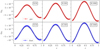	Fig. 6. DUSTYWAVE test. Same as in Fig. 5 but for the density perturbations.
In the text

	Fig. 7. DUSTYWAVE numerical convergence tests. L₂ norm as a function of the minimum cell size for the scheme using the Minmod slope limiter (blue squares), without predictor step (orange diamonds) and with AMR (green circles). The results are compared with a first-order slope (dashed line) and a second-order slope (dotted line).
In the text

	Fig. 8. SETTLING test on a uniform grid at level ℓ = 8 with millimeter-size dust grains. Dust ratio at t = 1 (red circles), 5 (blue circles), and 10 orbits (green circles) as a function of the altitude.
In the text

	Fig. 9. Comparison between multiple phase with 𝒩 = 5 (top) and an equivalent single phase (bottom) DUSTYDIFFUSE test. Dust ratio as a function of the position at t = 1 (red), t = 5 (green), t = 10 (blue) and t = 20 s (purple) compared with the exact solution (black solid lines).
In the text

	Fig. 10. CPU time t_CPU of the ten equivalent DUSTYDIFFUSE tests as a function of the number of species 𝒩.
In the text

	Fig. 11. MULTIGRAIN DUSTYWAVE test. The three panels show the evolution of the maximum amplitude of the perturbation for the dust densities (top), the gas density (middle), and the gas velocity (bottom). The K = 50 and K = 1000 dust phases are shown with blue and green circles respectively. The red circles represent the gas. The semi-analytic solution is given by the dashed black line.
In the text

	Fig. 12. MULTIGRAIN SETTLING test. Dust ratios and dust velocities (circles) of the ten phases of the SETTLING test after ten orbits compared with the numerical (dotted black lines) and analytic (black lines) one-species solution.
In the text

	Fig. 13. MULTIGRAIN SETTLING test. Dust density for the species j = 2, 4, 6, 8, and 10 in the (xy)-plane at t = 0, 1, 5, and 10 orbits.
In the text

	Fig. 14. MULTIGRAIN SETTLING test. Magnification of the dust front as a function of y for the j = 1 dust species (brown circles) compared with the one-species solution (dotted line). These dust grains are dragged by the gas, which is itself submitted to the cumulative back-reaction of all the other dust species through the gas, hence the difference is the one-species solution.
In the text

	Fig. 15. Ratio of the free-fall timescale of the mixture to the free-fall timescale of the gas. The red circle corresponds to the fiducial simulation with gas only, and the blue circles correspond to gas and dust mixtures for various dust ratios. The black solid line is the analytical solution.
In the text

	Fig. 16. Properties of the first Larson core when ρ_g ∼ 10⁻¹¹ g cm⁻³ for Col1, Col10, and Col100. The core mass, the dust mass ratio, and the formation time are shown as a function of the grain size (blue circles). The results are compared with the fiducial ColGAS simulation (dashed red lines). The top x-axis shows the initial Stokes number in the core St₀.
In the text

	Fig. 17. Radial profiles of the Col10 test. Top left: gas density. Top right: dust ratio. Bottom left: gas and dust velocities. Bottom right: stokes number. The horizontal green line corresponds to a dust-to-gas ratio of 1%.
In the text

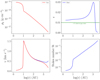	Fig. 18. Same as Fig.17, but for the Col100 test.
In the text

Current usage metrics show cumulative count of Article Views (full-text article views including HTML views, PDF and ePub downloads, according to the available data) and Abstracts Views on Vision4Press platform.

Data correspond to usage on the plateform after 2015. The current usage metrics is available 48-96 hours after online publication and is updated daily on week days.

Initial download of the metrics may take a while.

[1] Andre, P., Ward-Thompson, D., & Barsony, M. 2000, Protostars and Planets IV, 59 [Google Scholar]

[2] Ayliffe, B. A., Laibe, G., Price, D. J., & Bate, M. R. 2012, MNRAS, 423, 1450 [NASA ADS] [CrossRef] [Google Scholar]

[3] Barenblatt, G. 1952, Prikladnaya Matematika i Mekhanika, 16, 679 [Google Scholar]

[4] Bate, M. R., & Lorén-Aguilar, P. 2017, MNRAS, 465, 1089 [NASA ADS] [CrossRef] [Google Scholar]

[5] Berger, M. J., & Oliger, J. 1984, J. Comput. Phys., 53, 484 [NASA ADS] [CrossRef] [MathSciNet] [Google Scholar]

[6] Boss, A. P., & Bodenheimer, P. 1979, ApJ, 234, 289 [NASA ADS] [CrossRef] [Google Scholar]

[7] Chen, J.-W., & Lin, M.-K. 2018, MNRAS, 478, 2737 [NASA ADS] [CrossRef] [Google Scholar]

[8] Chiang, E. 2008, ApJ, 675, 1549 [CrossRef] [Google Scholar]

[9] Commerçon, B., Hennebelle, P., Audit, E., Chabrier, G., & Teyssier, R. 2008, A&A, 482, 371 [NASA ADS] [CrossRef] [EDP Sciences] [Google Scholar]

[10] Commerçon, B., Teyssier, R., Audit, E., Hennebelle, P., & Chabrier, G. 2011, A&A, 529, A35 [NASA ADS] [CrossRef] [EDP Sciences] [Google Scholar]

[11] Commerçon, B., Debout, V., & Teyssier, R. 2014, A&A, 563, A11 [NASA ADS] [CrossRef] [EDP Sciences] [Google Scholar]

[12] Compiègne, M., Verstraete, L., Jones, A., et al. 2011, A&A, 525, A103 [NASA ADS] [CrossRef] [EDP Sciences] [Google Scholar]

[13] Courant, R., Friedrichs, K., & Lewy, H. 1928, Mathematische Annalen, 100, 32 [Google Scholar]

[14] Courant, R., Isaacson, E., & Rees, M. 1952, Commun. Pure Appl. Math., 5, 243 [CrossRef] [Google Scholar]

[15] Dubois, Y., & Commerçon, B. 2016, A&A, 585, A138 [NASA ADS] [CrossRef] [EDP Sciences] [Google Scholar]

[16] Epstein, P. S. 1924, Phys. Rev., 23, 710 [NASA ADS] [CrossRef] [Google Scholar]

[17] Fromang, S., Hennebelle, P., & Teyssier, R. 2006, A&A, 457, 371 [NASA ADS] [CrossRef] [EDP Sciences] [Google Scholar]

[18] Gingold, R. A., & Monaghan, J. J. 1977, MNRAS, 181, 375 [Google Scholar]

[19] Godunov, S. K. 1959, Mat. Sb. (N.S.), 47, 271 [Google Scholar]

[20] González, M., Vaytet, N., Commerçon, B., & Masson, J. 2015, A&A, 578, A12 [NASA ADS] [CrossRef] [EDP Sciences] [Google Scholar]

[21] Harsono, D., Bjerkeli, P., & van der Wiel, M. H. D. 2018, Nat. Astron., 2, 646 [NASA ADS] [CrossRef] [Google Scholar]

[22] Harten, A. 1983, J. Comput. Phys., 49, 357 [NASA ADS] [CrossRef] [MathSciNet] [Google Scholar]

[23] Harten, A., Lax, D. P., & van Leer, B. 1983, SIAM Rev., 25, 35 [Google Scholar]

[24] Hennebelle, P. 2018, A&A, 611, A24 [NASA ADS] [CrossRef] [EDP Sciences] [Google Scholar]

[25] Hopkins, P. F., & Lee, H. 2016, MNRAS, 456, 4174 [NASA ADS] [CrossRef] [Google Scholar]

[26] Hutchison, M., Price, D. J., & Laibe, G. 2018, MNRAS, 476, 2186 [NASA ADS] [CrossRef] [Google Scholar]

[27] Laibe, G., & Price, D. J. 2011, MNRAS, 418, 1491 [NASA ADS] [CrossRef] [Google Scholar]

[28] Laibe, G., & Price, D. J. 2012, MNRAS, 420, 2365 [NASA ADS] [CrossRef] [Google Scholar]

[29] Laibe, G., & Price, D. J. 2014a, MNRAS, 440, 2136 [NASA ADS] [CrossRef] [Google Scholar]

[30] Laibe, G., & Price, D. J. 2014b, MNRAS, 440, 2147 [NASA ADS] [CrossRef] [Google Scholar]

[31] Laibe, G., & Price, D. J. 2014c, MNRAS, 444, 1940 [NASA ADS] [CrossRef] [Google Scholar]

[32] Larson, R. B. 1969, MNRAS, 145, 271 [NASA ADS] [CrossRef] [Google Scholar]

[33] Lax, P., & Wendroff, B. 1960, Commun. Pure Appl. Math., 13, 217 [CrossRef] [Google Scholar]

[34] Lin, M.-K., & Youdin, A. N. 2017, ApJ, 849, 129 [NASA ADS] [CrossRef] [Google Scholar]

[35] Lorén-Aguilar, P., & Bate, M. R. 2014, MNRAS, 443, 927 [NASA ADS] [CrossRef] [Google Scholar]

[36] Lorén-Aguilar, P., & Bate, M. R. 2015, MNRAS, 454, 4114 [NASA ADS] [CrossRef] [Google Scholar]

[37] Lucy, L. B. 1977, AJ, 82, 1013 [NASA ADS] [CrossRef] [Google Scholar]

[38] Marchand, P., Masson, J., Chabrier, G., et al. 2016, A&A, 592, A18 [NASA ADS] [CrossRef] [EDP Sciences] [Google Scholar]

[39] Marchand, P., Commercon, B., & Chabrier, G. 2018, A&A, 619, A37 [NASA ADS] [CrossRef] [EDP Sciences] [Google Scholar]

[40] Mathis, J. S., Rumpl, W., & Nordsieck, K. H. 1977, ApJ, 217, 425 [NASA ADS] [CrossRef] [Google Scholar]

[41] Masson, J., Teyssier, R., Mulet-Marquis, C., Hennebelle, P., & Chabrier, G. 2012, ApJS, 201, 24 [NASA ADS] [CrossRef] [Google Scholar]

[42] Pagani, L., Steinacker, J., Bacmann, A., Stutz, A., & Henning, T. 2010, Science, 329, 1622 [NASA ADS] [CrossRef] [PubMed] [Google Scholar]

[43] Price, D. J., & Laibe, G. 2015, MNRAS, 454, 2320 [NASA ADS] [CrossRef] [Google Scholar]

[44] Price, D. J., Wurster, J., & Nixon, C. 2017, Astrophysics Source Code Library [record ascl:1709.002] [Google Scholar]

[45] Roe, P. L. 1986, Annu. Rev. Fluid Mech., 18, 337 [Google Scholar]

[46] Rosdahl, J., & Teyssier, R. 2015, MNRAS, 449, 4380 [NASA ADS] [CrossRef] [Google Scholar]

[47] Rosdahl, J., Blaizot, J., Aubert, D., Stranex, T., & Teyssier, R. 2013, MNRAS, 436, 2188 [NASA ADS] [CrossRef] [Google Scholar]

[48] Saffman, P. G. 1962, J. Fluid Mech., 13, 120 [NASA ADS] [CrossRef] [Google Scholar]

[49] Sharma, P., Colella, P., & Martin, D. F. 2009, SIAM J. Sci. Comput., 32, 3564 [CrossRef] [Google Scholar]

[50] Sod, G. A. 1978, J. Comput. Phys., 27, 1 [NASA ADS] [CrossRef] [MathSciNet] [Google Scholar]

[51] Stoyanovskaya, O. P., Snytnikov, V. N., & Vorobyov, E. I. 2017, Astron. Rep., 61, 1044 [NASA ADS] [CrossRef] [Google Scholar]

[52] Stoyanovskaya, O. P., Vorobyov, E. I., & Snytnikov, V. N. 2018, Astron. Rep., 62, 455 [NASA ADS] [CrossRef] [Google Scholar]

[53] Teyssier, R. 2002, A&A, 385, 337 [NASA ADS] [CrossRef] [EDP Sciences] [Google Scholar]

[54] Teyssier, R., Fromang, S., & Dormy, E. 2006, J. Comput. Phys., 218, 44 [NASA ADS] [CrossRef] [Google Scholar]

[55] Tricco, S. T., Price, J. D., & Laibe, G. 2017, MNRAS, submitted [Google Scholar]

[56] Truelove, J. K., Klein, R. I., McKee, C. F., et al. 1997, ApJ, 489, L179 [NASA ADS] [CrossRef] [Google Scholar]

[57] van Leer, B. 1974, J. Comput. Phys., 14, 361 [NASA ADS] [CrossRef] [Google Scholar]

[58] van Leer, B. 1979, J. Comput. Phys., 32, 101 [Google Scholar]

[59] Vaytet, N., Commerçon, B., Masson, J., González, M., & Chabrier, G. 2018, A&A, 615, A5 [NASA ADS] [CrossRef] [EDP Sciences] [Google Scholar]

[60] Weingartner, J. C., & Draine, B. T. 2001, ApJ, 548, 296 [NASA ADS] [CrossRef] [Google Scholar]

[61] Youdin, A. N., & Goodman, J. 2005, ApJ, 620, 459 [NASA ADS] [CrossRef] [Google Scholar]

[62] Zhao, B., Caselli, P., Li, Z.-Y., et al. 2016, MNRAS, 460, 2050 [NASA ADS] [CrossRef] [Google Scholar]