| Issue |
A&A
Volume 625, May 2019
|
|
|---|---|---|
| Article Number | A68 | |
| Number of page(s) | 16 | |
| Section | Stellar structure and evolution | |
| DOI | https://doi.org/10.1051/0004-6361/201834965 | |
| Published online | 14 May 2019 | |
The CARMENES search for exoplanets around M dwarfs
Different roads to radii and masses of the target stars⋆
1
Hamburger Sternwarte, Gojenbergsweg 112, 21029 Hamburg, Germany
e-mail: This email address is being protected from spambots. You need JavaScript enabled to view it.
2
Departamento de Astrofísica, Centro de Astrobiología (CSIC-INTA), ESAC Campus, Camino Bajo del Castillo s/n, 28691 Villanueva de la Cañada, Madrid, Spain
3
Departamento de Física de la Tierra y Astrofísica and UPARCOS-UCM (Unidad de Física de Partículas y del Cosmos de la UCM), Facultad de Ciencias Físicas, Universidad Complutense de Madrid, 28040 Madrid, Spain
4
Instituto de Astrofísica de Canarias, Vía Láctea s/n, 38205 La Laguna, Tenerife, Spain
5
Departamento de Astrofísica, Universidad de La Laguna, 38206 La Laguna, Tenerife, Spain
6
Instituto Nacional de Astrofísica, Óptica y Electrónica, Luis Enrique Erro 1, Sta. Ma. Tonantzintla, Puebla, Mexico
7
Max-Planck-Institut für Astronomie, Königstuhl 17, 69117 Heidelberg, Germany
8
Centro de Astrobiología (CSIC-INTA), Carretera de Ajalvir km 4, 28850 Torrejón de Ardoz, Madrid, Spain
9
Institut de Ciències de l’Espai (CSIC-IEEC), Can Magrans s/n, Campus UAB, 08193 Bellaterra, Barcelona, Spain
10
Institut d’Estudis Espacials de Catalunya (IEEC), C/ Gran Capità 2-4, 08034 Barcelona, Spain
11
Institut für Astrophysik, Georg-August-Universität, Friedrich-Hund-Platz 1, 37077 Göttingen, Germany
12
Landessternwarte, Zentrum für Astronomie der Universtät Heidelberg, Königstuhl 12, 69117 Heidelberg, Germany
13
Instituto de Astrofísica de Andalucía (IAA-CSIC), Glorieta de la Astronomía s/n, 18008 Granada, Spain
14
Centro Astronómico Hispano-Alemán (CSIC-MPG), Observatorio Astronómico de Calar Alto, Sierra de los Filabres, 04550 Gérgal, Almería, Spain
15
School of Physics and Astronomy, Queen Mary, University of London, 327 Mile End Road, London E1 4NS, UK
16
Thüringer Landessternwarte Tautenburg, Sternwarte 5, 07778 Tautenburg, Germany
Received:
21
December
2018
Accepted:
25
March
2019
Abstract
Aims. We determine the radii and masses of 293 nearby, bright M dwarfs of the CARMENES survey. This is the first time that such a large and homogeneous high-resolution (R > 80 000) spectroscopic survey has been used to derive these fundamental stellar parameters.
Methods. We derived the radii using Stefan–Boltzmann’s law. We obtained the required effective temperatures Teff from a spectral analysis and we obtained the required luminosities L from integrated broadband photometry together with the Gaia DR2 parallaxes. The mass was then determined using a mass-radius relation that we derived from eclipsing binaries known in the literature. We compared this method with three other methods: (1) We calculated the mass from the radius and the surface gravity log g, which was obtained from the same spectral analysis as Teff. (2) We used a widely used infrared mass-magnitude relation. (3) We used a Bayesian approach to infer stellar parameters from the comparison of the absolute magnitudes and colors of our targets with evolutionary models.
Results. Between spectral types M0 V and M7 V our radii cover the range 0.1 R⊙ < R < 0.6 R⊙ with an error of 2–3% and our masses cover 0.09 ℳ⊙ < ℳ< 0.6ℳ⊙ with an error of 3–5%. We find good agreement between the masses determined with these different methods for most of our targets. Only the masses of very young objects show discrepancies. This can be well explained with the assumptions that we used for our methods.
Key words: stars: fundamental parameters / stars: low-mass / stars: late-type / stars: general
Table B.1 (stellar parameters) is only available at the CDS via anonymous ftp to cdsarc.u-strasbg.fr (130.79.128.5) or via http://cdsarc.u-strasbg.fr/viz-bin/qcat?J/A+A/625/A68
© ESO 2019
1. Introduction
The mass of a star is one of its most important properties. When trying to understand a star by itself and when isolating it from its environment, it is fundamental to stellar physics that the mass is the most influential parameter that determines almost exclusively all other properties throughout a star’s life. Moreover, should the star have a companion, the masses of both components determine the gravitational potential and their orbits. In particular, if the companion is a planet, the gravitational potential is dominated by the stellar mass, which is crucial to know if we want to measure the minimum mass, ℳP sin i, of the planet.
The latter is the situation that the CARMENES search faces in its quest to find Earth-mass planets. CARMENES (Calar Alto high-Resolution search for M dwarfs with Exo-earths with Near-infrared and optical Échelle Spectrographs) is a double channel spectrograph built to find Earth-mass planets around M dwarfs using the radial-velocity method (Quirrenbach et al. 2014). The visual channel of this spectrograph has a resolving power of R ≈ 95 000 and covers the wavelength range from 0.52 μm to 0.96 μm. Its near infrared channel has a resolving power of R ≈ 80 000 and covers the wavelength range from 0.96 μm to 1.71 μm. This spectrograph is operated at the 3.5 m telescope on Calar Alto, Spain, and has been taking data since January 2016 (Quirrenbach et al. 2016, 2018; Reiners et al. 2018a). So far CARMENES has been used in the discovery of several new planets (Reiners et al. 2018b; Kaminski et al. 2018; Ribas et al. 2018; Luque et al. 2018; Nagel et al. 2019). All of these discoveries estimated the mass of the host star with the same procedure that we present in this work, even though Reiners et al. (2018b), Kaminski et al. (2018), and Ribas et al. (2018) used slightly older data than those used in this work. However, an in-depth investigation of the validity of this method is still missing.
A widely used method to determine masses of M dwarfs directly is the observation of detached double-lined eclipsing binary systems (see, e.g., Andersen 1991; Torres et al. 2010; Torres 2013, for reviews). Accurately measuring the radial-velocity amplitudes of the components of such systems allows us to derive their stellar masses independently. Another method to measure the masses of M dwarfs dynamically are observations of astrometric binaries that are also visual or spectroscopic binaries (see, e.g., Quirrenbach et al. 2001; Benedict et al. 2016, and both their references), for which it is possible to reconstruct the orbits of the components.
For measuring stellar radii, eclipsing binaries can be used as well. The radii of their components and the inclination of the system can be determined from the eclipsing light curve (e.g., Torres & Ribas 2002; Ribas 2003; Clausen et al. 2009; Morales et al. 2009). For single stars, interferometry is used to directly measure the angular diameter (e.g., van Belle et al. 2009; Boyajian et al. 2012a,b; Ligi et al. 2016). Together with the distance, the physical radius can be inferred from the same dataset. However, it is difficult to apply this method to low-mass stars because they are small and faint, which requires high sensitivity and resolution to achieve acceptable accuracy. Some interferometric radius measurements of M dwarfs with uncertainties of 1–5% have been performed by Ségransan et al. (2003), Berger et al. (2006), Boyajian et al. (2012b), and von Braun et al. (2014).
On the other hand, because the fundamental techniques of measuring the mass and radius of isolated M dwarfs (or those with wide companions) are limited, well-calibrated empirical relationships are generally employed. This is an adequate solution if the stars are assumed to behave like statistical representatives of the sample on which these relations are based. It has the advantage that only the luminosity or magnitude in certain bands has to be measured to estimate the stellar mass. An early mass-luminosity relation for M dwarfs was provided by Henry & Donald (1993). Several other works (e.g., Delfosse et al. 2000; Benedict et al. 2016; Mann et al. 2019) provided up-to-date mass-magnitude relations for low-mass stars, calibrated for different parameter ranges. Additionally, relations connecting colors or other measurable quantities with the mass or radius that are not directly accessible have been established to determine missing parameters of stars in question (e.g., Mann et al. 2015). If there are, however, systematic differences between the samples used to determine any such empirical relation and the stars to be analyzed, then there is a bias in the results, which are based on such relations. Most prominently, the level of stellar activity may cause such a bias. For example, Caballero et al. (2010), Jackson et al. (2018), and Kesseli et al. (2018) reported inflated radii for young, magnetically active, or fast rotating stars.
Therefore, to obtain the mass ℳ of the CARMENES targets we would traditionally use, for example, a ℳ−MK relation (e.g., Delfosse et al. 2000) and an infrared magnitude. This was actually done in the first CARMENES-based planet analysis (Trifonov et al. 2018) and in the survey overview of Reiners et al. (2018a). Our new approach, however, is to use such relations only when unavoidable. Instead, we exploit as much information from the observations as possible and use all the measurements, including our spectra and up-to-date photometry and parallaxes, already obtained. We also investigate the accuracy with which we can measure the radius and mass of a star. This includes calculating individual error bars for every analyzed object. We finally confront our method with other methods (both new and traditional) using the same homogeneous data set.
In Sect. 2 we present the sample used in this work. In Sect. 3 we describe our method. In short, we combine several purely observational data sets (high-resolution spectroscopy, photometry, and trigonometric parallaxes) with only one computational model (synthetic spectra based on a grid of model atmospheres) and one fundamental relation (a mass-radius relation) to obtain luminosities, radii, and masses. In Sect. 4 we compare the results from our method with results obtained from other alternative methods. In Sects. 5 and 6 we finally discuss the results and draw conclusions for the future.
2. The sample
To date, the catalog of targets observed during guaranteed time observations (GTO) of the CARMENES spectrograph includes a total of 341 bright, nearby M dwarfs or M dwarf systems, for which CARMENES based results have been published, and we use 293 of these for the reasons outlined below.
In this work we based our mass and radius determinations on the spectral analysis of Passegger et al. (2016; 2018, see Sect. 3.2). We imposed the same requirements and only used those CARMENES spectra with a signal-to-noise ratio (S/N) of S/N > 75. Furthermore, as in Passegger et al. (2018, hereafter Pass18) we excluded targets with spectral line profiles that cannot be reproduced by a purely photospheric model, i.e., stars with signs of activity that significantly affect the profiles of the lines used by Pass18 for determining stellar parameters; see Tal-Or et al. (2018) and Fuhrmeister et al. (2018) for the impact of activity on CARMENES target stars. Finally, as in Pass18 we excluded fast rotators. All these criteria finally yield 293 stars.
Previously, however, different CARMENES GTO samples have been studied. Reiners et al. (2018a) presented the initial sample of 324 CARMENES targets without any presumable companion closer than 5 arcsec, while Baroch et al. (2018) added nine double-lined spectroscopic binaries discovered in the survey. Baroch et al. (2018) determined their minimum masses and radii using methods suitable for spectroscopic binaries, but we do not consider these nine binaries in this work because we are interested only in isolated M dwarfs (or those with wide companions). One of the original 324 targets was recently determined to be a close astrometric binary as well (to be discussed in a future publication) and we do not consider it in this work either. There can still be some very long-period, low-amplitude, single-lined spectroscopic binaries in our GTO sample that are yet to be discovered and did not pass our initial filters (Cortés-Contreras et al. 2017; Jeffers et al. 2018; Baroch et al. 2018). Another eight objects did not have any or not sufficient observations to reach enough S/N to be tabulated by Reiners et al. (2018a). Three of these1 were included in the sample of Díez Alonso et al. (2019), who studied the rotation periods of CARMENES targets. All of these eight objects except one2 were included in the study of Schöfer et al. (2019), who investigated the activity of the CARMENES targets. We, finally, included six3 of the eight new targets.
We present our sample in Table B.1. For each of the 293 M dwarfs, we provide for identification purposes the CARMENES identifier (Caballero et al. 2016), the Gliese or Gliese & Jahreiss name when available, or the discovery name otherwise; we also give the luminosity-class V spectral type (Alonso-Floriano et al. 2015, and references therein). A histogram of the spectral types of our sample is shown in Fig. 1.
 |
Fig. 1. Histogram of the spectral types (as determined by Alonso-Floriano et al. 2015, and references therein) of all 293 targets of our sample. The leftmost bin represents the only K7 V star in our sample. |
3. Our method
Our method is a multi-step process. In the first step in Sect. 3.1 we determine the luminosity from distance and photometry. In the second step in Sect. 3.2 we measure the effective temperature from the CARMENES spectra by fitting PHOENIX (Hauschildt & Baron 1999) synthetic spectra. In the third step in Sect. 3.3 we use Stefan–Boltzmann’s law to obtain the radius. To finally obtain the masses in Sect. 3.4, we introduce an empirical mass-radius relation to calculate the mass from the radius. These steps, along with those needed for the alternative methods, are sketched in Fig. 2.
 |
Fig. 2. Flowchart of our different roads to masses. |
3.1. Distances and luminosities
We determine the luminosities from apparent magnitudes and distances. For 285 of the 293 M dwarfs, we retrieve parallactic distances from the Gaia DR2 catalog (Gaia Collaboration 2018). For the remaining eight cases, which are not part of Gaia DR2 and are listed in Table B.1 together with a corresponding note, we retrieve parallactic distances from the astrometric analyses of van Altena et al. (1995, two stars4), van Leeuwen (2007, three stars5), and Finch & Zacharias (2016, two stars6), and derive spectrophotometric distances after applying the J-band absolute magnitude-spectral type relation given by Cortés-Contreras et al. (2017, one star7).
For every target star in the CARMENES input catalog Carmencita (Caballero et al. 2016), we collected apparent magnitudes in broadband passbands from a number of all-sky and ultra-wide surveys from the ultraviolet, through optical and near-infrared, to the mid-infrared. The integration of the spectral energy distribution (SED) of each CARMENES target allowed us to determine the bolometric luminosity L. In our case, we performed the integration with the Virtual Observatory SED Analyzer (VOSA; Bayo et al. 2008), the distances described above, and the SEDs built with photometric data from GALEX (FUV NUV; Morrissey et al. 2007), SDSS (ugriz; York et al. 2000), UCAC4 and APASS9 (BgVri; Zacharias et al. 2013; Henden et al. 2015), Tycho-2 (BT VT; Høg et al. 2000), Gaia DR2 (BP G RP; Gaia Collaboration 2018), CMC15 (r′; Muiños & Evans 2014), Pan-STARRS1 (grizy; Tonry et al. 2012), 2MASS (JHKs; Skrutskie et al. 2006), and AllWISE (W1 W2 W3 W4; Cutri 2014). The VOSA software uses the latest zero-point fluxes provided by the Filter Profile Service (Rodrigo et al. 2012), which can be found on their website8. We used synthetic photometry based on the BT-Settl models (Allard et al. 2012) for the ultraviolet flux blueward of the Johnson B band and for the mid- and far-infrared redward of WISE W4. At the considered effective temperatures, M dwarfs hardly emit any flux in these two wavelength regions. Therefore, the approximation of these two contributions to the luminosity are barely dependent on the models chosen as input to VOSA. Moreover, by using synthetic photometry for the ultraviolet we do not contaminate the photospheric flux with chromospheric flux from stellar activity. The resulting luminosities are listed in Table B.1. Typical relative errors of L are between 1 and 2%. More details on the photometry compilation and luminosity derivation including their errors will be provided in a separate publication.
3.2. Effective temperatures, surface gravities, and metallicities
We measured the photospheric parameters effective temperature Teff, surface gravity log g, and metallicity, denoted by the relative iron abundance [Fe/H] by fitting PHOENIX-ACES synthetic spectra (Husser et al. 2013) to the CARMENES spectra of the visual (VIS) channel as described in Passegger et al. (2016) and Pass18. In summary, this method has Teff and [Fe/H] as free parameters, but fixes log g by a Teff−log g relation from theoretical 5 Gyr isochrones of Baraffe et al. (1998). To analyze all 293 members of our sample described in Sect. 2, we repeated the analysis of Pass18 using the latest available CARMENES co-added (Zechmeister et al. 2018) VIS spectra that fulfill the requirements of Pass18 described above (cf. Sect. 2).
Pass18 presented the stellar photospheric parameters for 235 stars of our exoplanet survey. These authors used CARMENES VIS data for 234 targets and CAFE (Calar Alto Fiber-fed Echelle spectrograph) data for one star. We present in this work 59 new parameter sets derived from CARMENES spectroscopy, and update the parameters for 234 stars of Pass18 (omitting the binary mentioned in Sect. 2). The updated and Pass18 results agree within their fixed error bars (ΔTeff = 51 K, Δlog g = 0.07 dex, and Δ[Fe/H] = 0.16 dex). All results are listed in Table B.1.
There exist, however, alternative model atmospheres and synthetic spectra for M dwarfs, most prominently the BT-Settl models (Allard et al. 2012). When they are used in spectral analyses, the fit quality (see, e.g., Rojas-Ayala et al. 2012) is similar to the fit quality in Pass18. However, the resulting photospheric parameters typically differ. Most recently, Rajpurohit et al. (2018) determined effective temperatures for the CARMENES GTO targets listed in Reiners et al. (2018a) using the latest BT-Settl models, which are about 100–200 K smaller than ours. Describing these differences is beyond the scope of this paper and they will be investigated in a future publication. However, in order to assess an error estimate resulting from the use of one specific set of synthetic spectra we repeated our analysis described above using the latest, publicly available grid with varying metallicities, which are the 2011 BT-Settl models. We then found effective temperatures that are about 50 K (i.e., our ΔTeff) hotter for Teff ≲ 3700 K and up to about 200 K cooler for Teff ≳ 3700 K. Owing to error propagation, this means that for Teff ≲ 3700 K the derived radii and masses (see below) that are based on PHOENIX-ACES models, and radii and masses that are based on BT-Settl models would agree within our error bars. However, for higher Teff values, there would be a systematic offset between these derived quantities. Similarly, using the significantly and systematically differing Teff results from Rajpurohit et al. (2018) would also introduce a systematic offset in radii and masses beyond our error bars.
3.3. Radii
Using the effective temperature Teff and luminosity L from Sect. 3.1 we calculated the radius R using Stefan–Boltzmann’s law
 (1)
(1)
The error for R is then described by
 (2)
(2)
When explicitly expressing L by the distance d and the photometrically measured flux S via L = 4πd2 ⋅ S the radius becomes
 (3)
(3)
and thus
 (4)
(4)
In the era of satellite-based parallaxes, the relative error in distance Δd/d is negligible except for the very few stars without Gaia DR2 or HIPPARCOS parallaxes. Therefore, the main contributions to the relative error arise from the precision of the measured effective temperature, ΔTeff/Teff, and photometry ΔS/S, which are both typically between 1 and 2 %, yielding typical ΔR/R between 2 and 3 %.
Our sample has 11 stars in common with the sample of stars with interferometric radii presented by Boyajian et al. (2012b). We used the interferometric angular diameter corrected for limb darkening ΘLD given in Boyajian et al. (2012b), but use Gaia DR2 distances d when available to calculate an interferometric radius Rinterf via
 (5)
(5)
These Rinterf are listed in Table 1 along with the angular diameters and distances that we used. When we compared our spectroscopic radii with Rinterf we find good agreement for 9 of the common stars, as can be seen in Fig. 3. Six of our radii have error bars comparable to the error bars obtained from interferometry. For the remaining 5 stars, interferometry is more precise, as expected. Only the radii of the 2 targets Gl 411 (J11033+359) and Gl 412A (J11054+435), which are based on HIPPARCOS parallaxes, differ significantly beyond their respective error bars (see Sect. 5.2). The parallactic distances for the other 9 M dwarfs are based on Gaia DR2 data.
Radii of 11 stars of our sample with interferometric diameters measured by Boyajian et al. (2012b).
 |
Fig. 3. Radii determined using the spectroscopic Teff from Sect. 3.2, the bolometric luminosity from Sect. 3.1, and Stefan–Boltzmann’s law plotted against interferometric radii from Boyajian et al. (2012b). The two discussed outliers are Gl 411 and Gl 412A with Rinterf of 0.392 and 0.398 R⊙, respectively. |
3.4. Masses (ℳℳ−R)
We compiled a sample of 55 detached, double-lined, double-eclipsing, main-sequence M dwarf binaries from the literature (see Table B.2 and Fig. 4). We excluded pre-main-sequence stars in very young open clusters and very old stars in globular clusters. From the published masses and radii of these eclipsing binaries, we estimated the best linear fit (following Press et al. 2007) of the mass-radius relation and found for the radius and mass range given by Table B.2,
 (6)
(6)
or equivalently
 (7)
(7)
 |
Fig. 4. Masses and radii for the eclipsing binaries of Table B.2. Blue crosses indicate field stars, while turquoise crosses indicate, from left to right, the low-metallicity globular cluster members NGC 6362 V41 B (Kaluzny et al. 2015), M4 V65 B (Kaluzny et al. 2013), and M55 V54 B (Kaluzny et al. 2014). The red solid line shows our best linear fit. The increasingly darker green dashed lines represent isochrones for 0.2, 2, and 13 Gyr from BHAC15. |
Both fits have a non-reduced χ2 ≈ 0.02 translating into an rms ≈ 0.02 in solar units.
By excluding members of young clusters, the mass-radius relation is well defined for M dwarfs older than a few hundred million years. This is underlined by the comparison with mass-radius relations for ages between 0.2 and 13 Gyr from evolutionary models for solar metallicity by Baraffe et al. (2015, hereafter BHAC15), also shown in Fig. 4. The explanation of the small difference between models and observations is beyond the scope of this paper. However, the small spread between the isochrones demonstrates that our linear mass-radius relation can be treated independently of age. Furthermore, our sample in Table B.2 includes all known eclipsing binaries in the field, independent of metallicity. Yet, our mass-radius relation is well defined, and, therefore, we conclude that it does not significantly depend on metallicity either. Such metallicity independence of the mass-radius relation for low-mass stars is also frequently found in evolutionary models (see, e.g., Fig. 3 of del Burgo & Allende Prieto 2018). This is underlined by including three representative low-metallicity members of the open clusters M 4, M 55, and NGC 6362 in Fig. 4 (but not in the fits for Eqs. 6 and 7), which match our mass-radius relation very well.
The reasons for the intrinsic spread in the observed mass-radius relation and the comparison to theoretical models have been and are still being investigated elsewhere (e.g., Feiden & Chaboyer 2012; Korda et al. 2017; Tognelli et al. 2018; Parsons et al. 2018). As pointed out by Parsons et al. (2018), this spread sets a lower limit on the error bars for the masses obtained with this method. In any case, for this paper, we assume that eclipsing binaries are representative of our single-star sample, and we apply our mass-radius relation to derive masses.
In Table B.1 and for the remainder of this paper we label masses determined with this method as ℳℳ−R. As already mentioned in the introduction, these are the masses that we have been using for the planet discoveries of CARMENES. However, Kaminski et al. (2018) used the effective temperature from Pass18. Reiners et al. (2018b) and Ribas et al. (2018) additionally used the mass-radius relation from Casal (2014) and the distances listed in Gaia DR1 (Gaia Collaboration 2016) or as measured by HIPPARCOS (van Leeuwen 2007) for calculating the luminosity. As a consequence, the masses we list for these three planet hosts9 are about 5–8% higher than in the discovery papers. The largest contribution to this change is the update of the parallax and, hence, luminosity.
4. Comparison methods
4.1. Spectroscopic masses (ℳlog g)
If we use the surface gravity log g from Sect. 3.2, the mass is calculated via
 (8)
(8)
and its error is calculated via
 (9)
(9)
In practice, the error in log g dominates the error in ℳ. The precision of our radii ΔR/R is about 2–3% (cf. Sect. 3.3). It would require Δlog g ≲ 0.03 dex for both contributions to Eq. (9) to become of similar size. However, our current Δlog g = 0.07 dex is about twice as large. In Table B.1 and for the remainder of this paper we label the mass determined with this method as ℳ log g.
We compare ℳℳ−R from above with ℳ log g in Fig. 5. We find systematically lower ℳ log g values for the lowest (ℳℳ−R ≲ 0.2ℳ⊙) and highest (ℳℳ−R ≳ 0.5 ℳ⊙) ℳℳ−R values. In between, the ℳ log g values are higher than the ℳℳ−R values, and in particular for ℳℳ−R between 0.4 and 0.5 ℳ⊙ there is a large scatter without any correlation, except for the highest metallicities, which seem to form a curve with a sharp turn around 0.5 ℳ⊙.
 |
Fig. 5. Comparison of masses for all stars in Table B.1 using our two methods described in Sect. 4.1 on the y-axis and Sect. 3.4 on the x-axis. See Fig. A.1 for the same plot without error bars and linear axes. |
Furthermore, we reverse the calculation and obtain the surface gravity from ℳℳ−R and Stefan–Boltzmann’s radius of Sect. (3.3). We call this log gc and list this value in Table B.1 as well. When we compare the spectroscopic log g from Sect. 3.2 to this log gc in Fig. 6 we find, as expected, a similar behavior as above when comparing ℳℳ−R with ℳ log g: there is a large scatter in the mid-value regime but there are consistent results for the highest and lowest surface gravities, i.e., the least and most massive stars. And, again, the highest metallicity stars form a curve with less scatter than the other metallicities. This is a similar result as found by Pass18 in their Fig. 6, where some spectroscopic log g values deviate from literature values in a similar fashion. Also similar to Pass18 and as mentioned in Sect. 3.2, our log g is connected to Teff. This metallicity dependent connection causes systematic effects due to the underlying evolutionary models. In particular, the log g values for high-metallicity results are obtained by extrapolating from solar metallicity isochrones (Pass18).
To examine whether log gc is more reliable than log g, we compare our log gc with literature values in Fig. 7 to produce a similar plot as Fig. 6 of Pass18. When comparing Fig. 6 of Pass18 to our Fig. 7 we find an improvement. The values published by Maldonado et al. (2015) generally agree well with our log gc. The log g values derived from radii and masses published by Mann et al. (2015) show a linear correlation to ours, although its slope is smaller than unity. Only the log g values derived from radii and masses published by Gaidos & Mann (2014) show a very weak correlation to ours. Since the log g values that have recently been published by Rajpurohit et al. (2018) do not correlate with Pass18 or other literature values, we did not include these values in Fig. 7. When we now use log gc as an input for our spectral analysis described in Sect. 3.2 and keep it fixed, the resulting effective temperatures (and metallicities) do not change significantly and, therefore, neither do the radii nor the masses determined in Sect. 3.
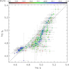 |
Fig. 6. Value of log gc calculated using ℳℳ−R from Sect. 3.4 and using R from Sect. 3.3 against the spectroscopic log g from Sect. 3.2. |
 |
Fig. 7. Value of log gc calculated using ℳℳ−R from Sect. 3.4 and using R from Sect. 3.3 against log g from the literature. |
Despite the large error bars inherent in calculating ℳ log g, and the problems described above, this method should not be generally dismissed. With precise input data as we have here, the error bars of ℳ log g become small enough so that the correlation in Fig. 5 becomes visible. However, since the ℳℳ−R masses have a much smaller error bar than the ℳ log g masses we decided to keep using ℳℳ−R.
4.2. Photometric masses (ℳM−Ks)
For M dwarfs well established mass-magnitude relations exist for infrared filters determined by Delfosse et al. (2000), Benedict et al. (2016), and most recently by Mann et al. (2019). The latter provided two variants: the first is independent of metallicity and the second one accounts for metallicities −0.4 < [Fe/H] < +0.3 when using their conservative validity range for metallicity. Both are valid for 4.5 mag < MKs < 10.5 mag, where MKs is the absolute magnitude in the 2MASS Ks band. Since they also compared their results extensively to the well-established (Mann et al. 2015) ℳ−MK relations of Delfosse et al. (2000) and Benedict et al. (2016) and found good (but not perfect, see below) agreement, and since we determined metallicities (Sect. 3.2) within the recommended range, we employed the metallicity dependent variant of Mann et al. (2019) by using their recommended software10. However, the metallicity independent relation yields only marginally different numbers. We list the resulting masses, ℳM−Ks, in Table B.1.
A comparison between our ℳℳ−R masses and the photometrically determined masses ℳM−Ks is given in Fig. 8. Except for individual outliers (which is discussed in Sect. 5.2), the two mass values agree very well. When we, alternatively, compare our ℳℳ−R values with the masses obtained from the two relations of Delfosse et al. (2000) and Benedict et al. (2016), we find disagreement of just beyond the size of our error bars for ℳℳ−R ≳ 0.3 ℳ⊙ but agreement otherwise. This is the same result described by Mann et al. (2019), who found discrepancies of about 10% between their values and the values obtained from the two previous relations above 0.3 ℳ⊙. For the remainder of this paper we use ℳℳ−R since differences between ℳℳ−R and ℳM−Ks are small.
 |
Fig. 8. Comparison of masses for all stars in Table B.1 using the method from Mann et al. (2019) as described in Sect. 4.2 on the y-axis and the method described in Sect. 3.4 on the x-axis. The metallicities are color coded as indicated. Obvious outliers, and stars discussed in reference to this figure in Sect. 5.2, are encircled: #1=Gl 411 (J11033+359), #3=GJ 4063 (J18346+401), #4=GJ 1235 (J19216+208), #8=1RXS J050156.7+010845 (J05019+011), #12=StKM 2-809 (J12156+526), and #14=K2-33 (J16102−193). See Fig. A.2 for a different comparison between the plotted values. |
As mentioned before, Trifonov et al. (2018) in their planet analysis and Reiners et al. (2018a) in their sample overview based their stellar masses on a mass-magnitude relation, but used a combination of the Delfosse et al. (2000) and Benedict et al. (2016) relations together with Gaia DR1 parallaxes. Therefore, our ℳM−Ks masses differ accordingly.
4.3. PARSEC-based masses (ℳP)
Another method we used consists of a Bayesian approach applied to the PARSEC library of stellar evolution models to infer stellar parameters, as performed by del Burgo & Allende Prieto (2018). We applied this technique to 262 targets from Table B.1, assuming solar metallicity, and with data for the SDSS r band, the 2MASS J band, and Gaia DR2 parallaxes to convert the apparent magnitudes J into MJ. The input parameters to feed the method were then MJ, r − J, and [Fe/H] = 0.0 ± 0.2 dex. The uncertainty in the iron-to-hydrogen ratio is reasonable since it reflects the range of [Fe/H] that we found in Sect. 3.2 (see also Fig. 5 of Pass18), and most of our targets belong to the thin disc (Cortés-Contreras 2016) for which this is a typical range.
A grid of PARSEC isochrones (version 1.2S; Bressan et al. 2012; Chen et al. 2014, 2015; Tang et al. 2014) were downloaded and arranged, where [Fe/H] ranges from −2.18 to 0.47 in steps of 0.05 dex, age spans from 2 Myr to 13.1 Gyr with steps of 0.1%, and the initial mass runs from 0.09 ℳ⊙ to the highest mass established by the corresponding stellar lifetime.
This method yields mass, radius, luminosity, metallicity, age, and all derivable parameters. For this work we only use mass and radius and list these in Table B.1 as RP and ℳP. The remaining results will be presented and discussed in a separate publication.
When we compare ℳℳ−R with ℳP in Fig. 9 we find good correlation except for five outliers. They are the very young objects K2-33 (J16102−193), 1RXS J050156.7+010845 (J05019+011,) and RX J0506.2+0439 (J05062+046), and the two stars RBS 365 (J02519+224) and Gl 15A (J00183+440). All of these targets are discussed in Sect. 5.2 below. However, all ℳP values are systematically slightly higher than ℳℳ−R. This means that the ℳP values are also systematically offset to the ℳM−Ks values in the same way.
 |
Fig. 9. Comparison of masses for all stars in Table B.1 using the method described in Sect. 4.3 on the y-axis and the method described in Sect. 3.4 on the x-axis. The metallicities are color coded as indicated. Obvious outliers, and stars discussed in reference to this figure in Sect. 5.2, are encircled: #6=Gl 15A (J00183+440), #8=1RXS J050156.7+010845 (J05019+011), #9=RX J0506.2+0439 (J05062+046), #14=K2-33 (J16102−193), and #18=RBS 365 (J02519+224). |
Once again, for the remainder of this paper we use ℳℳ−R since systematic differences between ℳℳ−R and ℳP do not change the overall picture, as described in Sect. 5.1.
5. Discussion
5.1. Sample properties
Having established a way to measure the masses of our targets, we investigate further statistical properties of our sample. When we use our results and produce a Hertzsprung–Russell diagram (HRD) in Fig. 10, we find all targets on the main sequence except for a few outliers. Most of these outliers are young. This is discussed on a case-by-case basis below.
 |
Fig. 10. Hertzsprung–Russell diagram using L from Sect. 3.1 and Teff from Sect. 3.2. The metallicities are color coded as indicated. For comparison we plot isochrones for 0.2, 2, and 13 Gyr (in increasingly darker green) from BHAC15. Obvious outliers, and stars discussed in reference to this figure in Sect. 5.2, are encircled: #1=Gl 411 (J11033+359), #2=Gl 412A (J11054+435), #4=GJ 1235 (J19216+208), #5=2M J06572616+7405265 (J06574+740), #7=RX J0447.2+2038 (J04472+206), #8=1RXS J050156.7+010845 (J05019+011), #10=G 234-057 (J09133+688), #11=TYC 3529-1437-1 (J18174+483), #12=StKM 2-809 (J12156+526), #13=GJ 9520 (J15218+209), #14=K2-33 (J16102−193), #15=Gl 745A (J19070+208), #16=Gl 745B (J19072+208), #17=Gl 465 (J12248−182), and #20=LP 022-420 (J15499+796). Outliers #12 and #13 lie almost on top of each other. See Fig. A.3 for the same plot but using the pseudo equivalent width |

Furthermore, when we plot Teff against the mass of the star we find the relation shown in Figs. 11 and 12. While there is a large spread, the distribution is well consistent with the isochrones by BHAC15. Again, we can identify outliers, most of which are young or active, and all of these cases are discussed below. While the HRD only compares our independently determined luminosities L and effective temperatures Teff, Fig. 11 directly shows the results of our method described in Sect. 3.4.
 |
Fig. 11. Values of ℳℳ−R from Sect. 3.4 plotted against Teff from Sect. 3.2. The metallicities are color coded as indicated. For comparison we plot isochrones for 0.2, 2, and 13 Gyr (in increasingly darker green) from BHAC15. Obvious outliers, and stars discussed in reference to this figure in Sect. 5.2, are encircled: #4=GJ 1235 (J19216+208), #5=2M J06572616+7405265 (J06574+740), #7=RX J0447.2+2038 (J04472+206), #8=1RXS J050156.7+010845 (J05019+011), #10=G 234-057 (J09133+688), #11=TYC 3529-1437-1 (J18174+483), #12=StKM 2-809 (J12156+526), #13=GJ 9520 (J15218+209), #14=K2-33 (J16102−193), #15=Gl 745A (J19070+208), #16=Gl 745B (J19072+208), #17=Gl 465 (J12248−182), #18=RBS 365 (J02519+224), #19=RX J1417.3+4525 (J14173+454), and #20=LP 022-420 (J15499+796). Outliers #12 and #13 lie almost on top of each other. |
 |
Fig. 12. Same as Fig. 11, but using the pseudo equivalent width |


Finally, when we plot the bolometric luminosity from Sect. 3.1 against the mass of the star to create a (bolometric) mass-luminosity relation we obtain Fig. 13. Again it is well consistent with the isochrones by BHAC15. When we fit a power law to these data for 0.1 ℳ⊙ < ℳℳ−R < 0.5 ℳ⊙ we find a flat power law of
 (10)
(10)
which deviates from power laws for L−ℳ relations that average the whole main sequence yielding exponents of at least three. However, this agrees with results obtained for very low-mass stars that show a flattening of this power law at the bottom of the main sequence. This flattening can be seen already in, for example, Torres et al. (2010) or del Burgo & Allende Prieto (2018). As a recent example, Eker et al. (2018, and similarly the references therein) have derived a comparable exponent of 2.028 ± 0.135 for 0.179 ℳ⊙ < ℳℳ< 0.45 ℳ⊙. For ℳℳ−R ≳ 0.5 ℳ⊙ the relation in Fig. 13 clearly required a different exponent, but our high-mass range is too small to fit a reliable second power law.
 |
Fig. 13. Mass-luminosity relation using L from Sect. 3.1 and ℳℳ−R from Sect. 3.4. The metallicities are color coded as indicated. For comparison we plot isochrones for 0.2, 2, and 13 Gyr (dashed lines in increasingly darker green) from BHAC15. The red solid line indicates the fit we obtained in Eq. (10) Obvious outliers, and stars discussed in reference to this figure in Sect. 5.2, are encircled: #4=GJ 1235 (J19216+208), #7=RX J0447.2+2038 (J04472+206), #8=1RXS J050156.7+010845 (J05019+011), #10=G 234-057 (J09133+688), #11=TYC 3529-1437-1 (J18174+483), #12=StKM 2-809 (J12156+526), and #14=K2-33 (J16102−193). |
5.2. Outliers
Most of the outliers discussed in this section are young objects. They either belong to young associations or to young moving groups. Our ℳℳ−R values, however, are based on the assumption that the stars are older than a few hundred million years (cf. Sect. 3.4). The ℳℳ−R values that we list for these young objects should be treated accordingly. As Pass18 have already concluded, their effective temperatures are generally not affected by this assumption. Under the further assumption that the luminosity is not affected much either, the radii we list are not affected much by any assumptions regarding ages either. In other words, in cases in which we list or show a mass that is too high, we also derive a similarly large radius (cf. Eqs. 6 and 7), which may be expected for young objects.
Another set of the targets listed below are outliers and at the same time, some of their entries in at least one of the photometric catalogs are marked as being of bad quality. If such systematic errors were accounted for, our error bars would be increased significantly.
5.2.1. Data-based reasons
We first eliminate all outliers from our discussion that have data-based reasons for their designation as outliers because we do not wish to misidentify physical reasons.
#1=Gl 411 (J11033+359) and #2=Gl 412A (J11054+435). For these two stars we obtain different radii than measured interferometrically (cf. Sect. 3.3). Both are missing in the latest Gaia catalog, therefore we use parallaxes from the HIPPARCOS measurements. However, when comparing Eqs. (3) and (5) it is obvious that the distance does not cause a mismatch between the two different methods of computing radii. We confirm that by using the Gaia distance of Gl 412B for Gl 412A since both form a common proper motion pair. The values R and Rinterf both changed slightly, but the data point in Fig. 3 only moved parallel to the 1–1-line, as expected.
Both stars have very reliable measurements of their effective temperatures since their fits described in Sect. 3.2 are of high quality. Furthermore, both Teff agree well with the recent measurements of Mann et al. (2015) and Rajpurohit et al. (2018). Therefore, the reason for the mismatch to the very reliable interferometric radii must lie in the photometry. As a test, we took three stars from Table 1 that are in Gaia DR2 (Gl 15A, Gl 880 and Gl 699) and for which we obtain good results using Gaia parallaxes and photometry (cf. Sect. 3.3). But for this test we ignored all the Gaia bands BP, G, and RP, and calculated the luminosities with the remaining photometry. Using VOSA, we obtained different luminosities and, hence, radii that no longer agreed with their interferometric counterparts. This is because the Gaia filters anchor the SED very reliably in the optical while 2MASS and AllWISE anchor the SED in the infrared. In particular Gl 15A, which has unreliable 2MASS photometry (see below), showed the largest change in the test.
As a consequence of its uncertain luminosity, radius, and mass, Gl 411 also appears below the main sequence in the HRD in Fig. 10 and is a mild outlier in Fig. 8. In addition to not having Gaia magnitudes, Gl 411 has also 2MASS and AllWISE magnitudes of poor quality because of its brightness. In both catalogs Gl 411 is listed to have magnitudes with low quality flags (DCD in 2MASS and UUAA in AllWISE). As described above, our error bars would have to be larger.
#3=GJ 4063 (J18346+401). This is an outlier when comparing ℳℳ−R to the absolute Ks band magnitude (cf. Fig. A.5). It is also one of the outliers when comparing ℳℳ−R with ℳM−Ks in Fig. 8. The reason for the deviations is the poor Ks-band photometry as indicated by the 2MASS quality flags (AAU).
#4=GJ 1235 (J19216+208). This object is an outlier in the HRD (Fig. 10), when plotting mass against effective temperature in Fig. 11 and in the L − ℳℳ−R plot in Fig. 13. However, we cannot explain this except by pointing out that this is a relatively faint, high proper motion star located in a crowded field where photometric contamination by background sources cannot be excluded.
#5=2MASS J06572616+7405265 (J06574+740). This object does not have a space-based parallax. We use the value obtained with the United States Naval Observatory Robotic Astrometric Telescope (Finch & Zacharias 2016), which is the only published trigonometric parallax and has a large relative error of 11%. Despite its large error bar, it is an outlier in the HRD (Fig. 10), and when plotting mass against effective temperature in Fig. 11. However, as an X-ray source (Haakonsen & Rutledge 2009) this is an active star (Ansdell et al. 2015; Schöfer et al. 2019), but we attribute its deviation in the diagrams instead to a wrong parallactic distance (d = 26 ± 3 pc). In the literature, there have been at least four additional distance determinations from photometry and spectroscopy (Lépine & Gaidos 2011; Lépine et al. 2013; Cortés-Contreras 2016), and they all point toward a closer distance in the range d = 14.0−19.6 pc, which would lead to a luminosity and mass consistent with its measured effective temperature. We expect the next Gaia release to improve the precision of its luminosity and to help clarify its nature.
#6=Gl 15A (J00183+440). When plotting mass versus the J magnitude (Fig. A.6) this object is a mild outlier. However, it is also too bright in the infrared to have reliable 2MASS magnitudes as indicated by their quality flags (DCE).
5.2.2. Young age-based reasons
#7=RX J0447.2+2038 (J04472+206). This is one of the outliers in the HRD (Fig. 10) and when comparing mass against Teff in Figs. 11 and 12. It is very active (Ishioka et al. 2014; Jeffers et al. 2018; Tal-Or et al. 2018), and Cortés-Contreras (2016) identified this object as a candidate member of the young disc population.
#8=1RXS J050156.7+010845 (J05019+011) and #9=RX J0506.2+0439 (J05062+046). The first is an outlier in all plots. It was identified by Schlieder et al. (2012a) to be a member of the β Pictoris moving group and, hence, very young. The second is a mild outlier and was identified by Schlieder et al. (2012b) as a candidate member of β Pictoris as well. These are two of the outliers in Fig. 9 comparing ℳP to ℳℳ−R. Their corresponding masses differ by about 30%. For the former the PARSEC-based method (cf. Sect. 4.3) yields for ℳP = 0.38 ± 0.08 ℳ⊙ an age of τ = 36 ± 16 Myr. For the latter the method yields for ℳP = 0.35 ± 0.07 ℳ⊙ an age of τ = 38 ± 17 Myr. Both ages are similar to the currently assumed age of β Pictoris of τ = 25 ± 3 Myr (e.g., Messina et al. 2016; Shkolnik et al. 2017).
#10=G 234-057 (J09133+688) and #11=TYC 3529-1437-1 (J18174+483). Both stars are noticeable outliers in almost all plots. However, both are young and candidate members of the AB Doradus association. The first was listed as a candidate by Schlieder et al. (2012b), and the second by Kastner et al. (2017). The second is also an active star discussed in Fuhrmeister et al. (2018).
#12=StKM 2-809 (J12156+526). This is an outlier in the L − ℳℳ−R plot in Fig. 13 and the HRD (Fig. 10). But again, this is an active (Stephenson 1986; Tal-Or et al. 2018), young star, which was identified as a candidate member of the Ursa Major moving group (Cortés-Contreras 2016).
#13=GJ 9520 (J15218+209). This is an outlier in almost every plot (e.g., in the HRD in Fig. 10), although not always an obvious one. It is an active (Fuhrmeister et al. 2018) and young star belonging to the Local Association (Tetzlaff et al. 2011).
#14=K2-33 (J16102−193). This is a pre-main-sequence star in the Upper Scorpius OB association. Its age is estimated to be between 5 and 20 Myr (David et al. 2016; Mann et al. 2016). It is a very obvious outlier in almost all plots. We measure unrealistic masses above 0.8 ℳ⊙ with all methods except that for obtaining ℳP described in Sect. 4.3. Therefore, it appears as one of the outliers in Fig. 9. The PARSEC-based method yields ℳP = 0.43 ± 0.10ℳ⊙ and at the same time an age of τ = 8.0 ± 3.5 Myr. Furthermore, it is by far the most distant target, and at a distance of d ≈ 140 pc located in Upper Scorpius, extinction can no longer be neglected.
5.2.3. Examples of possible surprising results
While the stars discussed in this section are not obvious outliers, they demonstrate certain physical effects that can result in unexpected masses or radii. Furthermore, these stars are only examples and not a comprehensive list. In particular the plots involving Teff (Figs. 10, 11 and 12) show a natural spread (as already described by Pass18), and the decision on which star is an outlier in these plots would require a non-trivial definition of a criterion.
#15=Gl 745A (J19070+208) and #16=Gl 745B (J19072+208). Both components of the wide binary system LDS 1017 are slightly below the main sequence in the HRD (Fig. 10). We also measure high effective temperatures for their derived masses when comparing these two parameters in Fig. 11. Together with very low activity they show a behavior akin to subdwarfs. Our derived [Fe/H] = −0.20 ± 0.16 dex and [Fe/H] = −0.23 ± 0.16 dex, respectively, also point toward low-metallicity objects. Furthermore, Mann et al. (2015) derived for Gl 745A an even lower metallicity of [Fe/H] = −0.33 ± 0.08 dex, and Houdebine (2008) already classified both components as subdwarfs.
#17=Gl 465 (J12248−182). As the previous two stars, this isolated star is below the main sequence in the HRD and has a very high effective temperature for its derived mass (see Fig. 11). We measure [Fe/H] = −0.17 ± 0.16 dex for this object. This metallicity is still too high to call it a subdwarf as it is still consistent with the solar. However, Maldonado et al. (2015) measured an even lower metallicity of [Fe/H] = −0.33 ± 0.09 dex for this star.
#18=RBS 365 (J02519+224), #19=RX J1417.3+4525 (J14173+454) and #20=LP 022-420 (J15499+796). These three stars are mild outliers in the HRD (Fig. 10) or when plotting mass against Teff (Figs. 11 and 12). These, however, are active stars that have, for instance, log LHα/Lbol > −4 (Schöfer et al. 2019). The latter two are also in the CARMENES radial-velocity-loud sample discussed by Tal-Or et al. (2018).
5.3. How do the masses differ?
Overall, all methods in determining masses yield consistent results, even when using log g in order to obtain ℳ log g.
The largest amount of information is used in the construction of ℳℳ−R (Sect. 3.4) and in the construction of ℳ log g (Sect. 4.1). The latter does not even use any empirical relation, however, it yields the largest error bars. Both ℳℳ−R and ℳM−Ks (Sect. 4.2) use an empirical relation. However, the ℳ−R relation is more fundamental than the mass-magnitude relation. Mass and radius are fundamentally connected via the hydrostatics of a star, whereas a magnitude is an “arbitrary” portion of the SED. It is not fundamentally obvious that the luminosity within a restricted wavelength range uniquely relates to the mass of a star. Of course, these relations are well established and have been working very well (not to mention that they only require photometry and no spectroscopy). After all, the infrared magnitudes are representative of the luminosity of a star since similar relations between near-infrared magnitudes and luminosity are also well established, and an ℳ−L relation is similarly fundamental as an ℳ−R relation. In any case, our work can be considered an independent confirmation of the mass-magnitude relations of Mann et al. (2019); Benedict et al. (2016), or Delfosse et al. (2000).
It follows from the above discussion on the outliers that the age of a star also plays a significant role in testing the validity of any method intended for obtaining its mass and radius. All of these, except the PARSEC-based masses ℳP (Sect. 4.3), assume an age of at least a few hundred megayears, i.e., that the stars have left the Hayashi track and reached the main sequence. Our spectral analysis (Sect. 3.2 and Pass18) assumes for the log g determination an age of 5 Gyr, which directly enters the spectroscopic mass ℳ log g. Both the mass-radius based masses ℳℳ−R and the photometric masses ℳM−Ks use empirical relations based on samples of old stars. This is in turn an advantage of the PARSEC-based masses ℳP because, for example, the GTO targets of the β Pictoris moving group and the Upper Scorpius OB association have significantly lower ℳP values than all the other masses. At the same time the method for obtaining ℳP yields young ages for these sources. However, a detailed investigation of the validity and consequences of the combined determination of all parameters of M dwarfs (and the CARMENES targets in particular) using this method is beyond the scope of this paper and will be discussed in a separate publication. Therefore, we do not list the ages determined with this method except for the few examples above. On the other hand, old stars such as the potential subdwarfs mentioned above do not pose a problem for our method. In particular, as described in Sect. 3.4, our mass-radius relation does not differ for different ages above a few hundred million years, nor can we infer a metallicity dependence down to metallicities of globular clusters.
Besides the age constraints inherent in the different methods, there are further biases that enter some of the methods as already indicated in the introduction. Both ℳℳ−R and ℳM−Ks use empirical relations based on binaries. However, the mass-radius relation for ℳℳ−R uses close binaries, while the mass-luminosity relation for ℳM−Ks is measured using wide binaries. The latter is certainly a better representation for isolated M dwarfs, i.e., our targets. If the former suffers from, for example, inflated radii then there is a systematic difference between ℳℳ−R and ℳM−Ks. Such inflated radii have been reported (e.g., Jackson et al. 2018; Kesseli et al. 2018, and for eclipsing binaries by Parsons et al. 2018), but only for young, magnetically active, or fast-rotating stars. Our sample, however, mostly includes old, inactive, and slowly rotating stars (see Sect. 2). But if such a bias exists within the mass-radius relation derived in Sect. 3.4, it introduces an offset in our ℳℳ−R values. As shown in Sect. 4.2 we find no offset between ℳℳ−R and ℳM−Ks, indicating no systematic difference between the mass-radius relation and the mass-magnitude relation, or the samples on which they are based.
Finally, as described in Sect. 3.2, the choice of a specific set of synthetic spectra in our spectral analysis may introduce another systematic offset on the order of our ΔTeff/Teff errors, or larger. But again, the agreement of our ℳℳ−R with the ℳM−Ks that we observe indicates that we did not introduce such a systematic offset.
6. Conclusions
We have derived radii and masses with individual error bars for 293 of the CARMENES GTO M dwarfs. In particular, for measuring the masses, we used several methods and compared them. For typical field stars that are not young, we list consistent masses with all methods. For our main method we list radii R that typically have errors of 2–3%, and masses ℳℳ−R that typically have errors of 3–5% (cf. Fig. 14). Systematic uncertainties on the order of the error bars, however, cannot be fully excluded.
 |
Fig. 14. Histograms of the errors of R and ℳℳ−R. |
For young stars, ℳℳ−R and ℳM−Ks are not suitable since the applicable empirical relations are derived for old stars (and cannot easily be adapted for young stars). Therefore, ℳℳ−R and ℳM−Ks for any young star in our sample (and not only for the outliers discussed in Sect. 5.2) should be used with care. The identification of all young stars, or determining their membership in young moving groups, should it exist, is beyond the purpose of this paper and will be published in the future. Similarly, an age determination of any star (not only those of our sample) is challenging. For example, Veyette & Muirhead (2018) derived ages for some of the CARMENES targets. On the other hand, ℳP is not restricted to a single age, and ages along with ℳP can be determined simultaneously as described in Sect. 4.3. Finally, when age estimates are available, our method of obtaining log g will be able to use isochrones for the appropriate age. Then our ℳ log g is also an option, at least when we will be able to reduce the error bars of log g to be smaller than the current 0.07 dex, and when systematic effects of theoretical isochrones can be reduced.
Our methods for measuring R and ℳℳ−R work best for a field star of at least a few hundred million years when we can spectroscopically determine a reliable Teff, when the parallax of the object is based on Gaia DR2, and when L is well anchored by Gaia and near-infrared photometry. Then, we can determine for the target with the latest spectral type in our sample, the M7 V object Teegarden’s star R = 0.107 ± 0.004 R⊙ and ℳℳ−R = 0.089 ± 0.009 ℳ⊙, while we determine for our M0.0 V targets average values R = 0.566 ± 0.016 R⊙ and ℳℳ−R = 0.574 ± 0.021 ℳ⊙.
J15474−108 (GJ 3916), J18198−019 (Gl 710) and J20556−140S (Gl 810B).
J18198−019 (Gl 710).
J04219+213 (K2-155), J08409−234 (Gl 317), J09143+526 (Gl 338A), J15474−108 (GJ 3916), J18198−019 (Gl 710) and J20556−140S (Gl 810B).
J22020−194 (Gl 843) and J18224+620 (GJ 1227).
J07274+052 (Gl 273), J11033+359 (Gl 411) and J11054+435 (Gl 412A).
J06574+740 (2M J06572616+7405265) and J09133+688 (G 234-057).
J06396−210 (LP 780-032).
J16167+672S (Gl 617A), J17578+046 (Gl 699), J1919+051N (Gl 752A).
Acknowledgments
We thank the anonymous referee for a very quick and very constructive report. Furthermore, we thank T. Boyajian and A. W. Mann for helpful discussions during the preparation of this manuscript. CARMENES is an instrument for the Centro Astronómico Hispano-Alemán de Calar Alto (CAHA, Almería, Spain). CARMENES is funded by the German Max-Planck-Gesellschaft (MPG), the Spanish Consejo Superior de Investigaciones Científicas (CSIC), the European Union through FEDER/ERDF FICTS-2011-02 funds, and the members of the CARMENES Consortium (Max-Planck-Institut für Astronomie, Instituto de Astrofísica de Andalucía, Landessternwarte Königstuhl, Institut de Ciències de l’Espai, Institut für Astrophysik Göttingen, Universidad Complutense de Madrid, Thüringer Landessternwarte Tautenburg, Instituto de Astrofísica de Canarias, Hamburger Sternwarte, Centro de Astrobiología and Centro Astronómico Hispano-Alemán), with additional contributions by the Spanish Ministry of Science through projects AYA2016-79425-C3-1/2/3-P, ESP2016-80435-C2-1-R, AYA2015-69350-C3-2-P, and AYA2018-84089, the Spanish Ministerio de Educación y Formación Profesional through fellowship FPU15/01476, the German Science Foundation through the Major Research Instrumentation Programme and DFG Research Unit FOR2544 “Blue Planets around Red Stars”, the Klaus Tschira Stiftung, the states of Baden-Württemberg and Niedersachsen, and by the Junta de Andalucía. CdB acknowledges the funding of his sabbatical position through the Mexican national council for science and technology (CONACYT grant CVU No. 448248). This publication makes use of VOSA, developed under the Spanish Virtual Observatory project, the VizieR catalog access tool (Ochsenbein et al. 2000) and the SIMBAD database (Wenger et al. 2000), operated both at CDS, Strasbourg, France, and the interactive graphical viewer and editor for tabular data TOPCAT (Taylor 2005)
References
- Allard, F., Homeier, D., & Freytag, B. 2012, Philos. Trans. R. Soc. London Ser. A, 370, 2765 [Google Scholar]
- Alonso-Floriano, F. J., Morales, J. C., Caballero, J. A., et al. 2015, A&A, 577, A128 [NASA ADS] [CrossRef] [EDP Sciences] [Google Scholar]
- Andersen, J. 1991, A&ARv, 3, 91 [NASA ADS] [CrossRef] [Google Scholar]
- Ansdell, M., Gaidos, E., Mann, A. W., et al. 2015, ApJ, 798, 41 [Google Scholar]
- Baraffe, I., Chabrier, G., Allard, F., & Hauschildt, P. H. 1998, A&A, 337, 403 [NASA ADS] [Google Scholar]
- Baraffe, I., Homeier, D., Allard, F., & Chabrier, G. 2015, A&A, 577, A42 [NASA ADS] [CrossRef] [EDP Sciences] [Google Scholar]
- Baroch, D., Morales, J. C., Ribas, I., et al. 2018, A&A, 619, A32 [NASA ADS] [CrossRef] [EDP Sciences] [Google Scholar]
- Bass, G., Orosz, J. A., Welsh, W. F., et al. 2012, ApJ, 761, 157 [NASA ADS] [CrossRef] [Google Scholar]
- Bayo, A., Rodrigo, C., Barrado, Y., & Navascués, D. 2008, A&A, 492, 277 [NASA ADS] [CrossRef] [EDP Sciences] [Google Scholar]
- Becker, A. C., Agol, E., Silvestri, N. M., et al. 2008, MNRAS, 386, 416 [NASA ADS] [CrossRef] [Google Scholar]
- Bender, C. F., Mahadevan, S., Deshpande, R., et al. 2012, ApJ, 751, L31 [NASA ADS] [CrossRef] [Google Scholar]
- Benedict, G. F., Henry, T. J., Franz, O. G., et al. 2016, AJ, 152, 141 [NASA ADS] [CrossRef] [Google Scholar]
- Berger, D. H., Gies, D. R., McAlister, H. A., et al. 2006, ApJ, 644, 475 [NASA ADS] [CrossRef] [Google Scholar]
- Blake, C. H., Torres, G., Bloom, J. S., & Gaudi, B. S. 2008, ApJ, 684, 635 [NASA ADS] [CrossRef] [Google Scholar]
- Bouchy, F., Pont, F., Melo, C., et al. 2005, A&A, 431, 1105 [NASA ADS] [CrossRef] [EDP Sciences] [Google Scholar]
- Boyajian, T. S., McAlister, H. A., van Belle, G., et al. 2012a, ApJ, 746, 101 [NASA ADS] [CrossRef] [Google Scholar]
- Boyajian, T. S., von Braun, K., van Belle, G., et al. 2012b, ApJ, 757, 112 [NASA ADS] [CrossRef] [Google Scholar]
- Bressan, A., Marigo, P., Girardi, L., et al. 2012, MNRAS, 427, 127 [NASA ADS] [CrossRef] [Google Scholar]
- Caballero, J. A., Montes, D., Klutsch, A., et al. 2010, A&A, 520, A91 [NASA ADS] [CrossRef] [EDP Sciences] [Google Scholar]
- Caballero, J. A., Cortés-Contreras, M., & Alonso-Floriano, F. J. 2016, 19th Cambridge Workshop on Cool Stars, Stellar Systems, and the Sun (CS19), 148 [Google Scholar]
- Carter, J. A., Fabrycky, D. C., Ragozzine, D., et al. 2011, Science, 331, 562 [NASA ADS] [CrossRef] [PubMed] [Google Scholar]
- Casal, E. 2014, Master’s Thesis (Spain: Universidad de La Laguna) [Google Scholar]
- Chen, Y., Girardi, L., Bressan, A., et al. 2014, MNRAS, 444, 2525 [NASA ADS] [CrossRef] [Google Scholar]
- Chen, Y., Bressan, A., Girardi, L., et al. 2015, MNRAS, 452, 1068 [NASA ADS] [CrossRef] [Google Scholar]
- Clausen, J. V., Bruntt, H., Claret, A., et al. 2009, A&A, 502, 253 [NASA ADS] [CrossRef] [EDP Sciences] [Google Scholar]
- Cortés-Contreras, M. 2016, PhD Thesis (Spain: Universidad Compultense de Madrid) [Google Scholar]
- Cortés-Contreras, M., Béjar, V. J. S., Caballero, J. A., et al. 2017, A&A, 597, A47 [NASA ADS] [CrossRef] [EDP Sciences] [Google Scholar]
- Creevey, O. L., Benedict, G. F., Brown, T. M., et al. 2005, ApJ, 625, L127 [NASA ADS] [CrossRef] [Google Scholar]
- Cutri, R. M. 2014, VizieR Online Data Catalog, II/328 [Google Scholar]
- David, T. J., Hillenbrand, L. A., Petigura, E. A., et al. 2016, Nature, 534, 658 [NASA ADS] [CrossRef] [PubMed] [Google Scholar]
- del Burgo, C., & Allende Prieto, C. 2018, MNRAS, 479, 1953 [NASA ADS] [CrossRef] [Google Scholar]
- Delfosse, X., Forveille, T., Ségransan, D., et al. 2000, A&A, 364, 217 [NASA ADS] [Google Scholar]
- Díez Alonso, E., Caballero, J. A., Montes, D., et al. 2019, A&A, 621, A126 [NASA ADS] [CrossRef] [EDP Sciences] [Google Scholar]
- Dittmann, J. A., Irwin, J. M., Charbonneau, D., et al. 2017, ApJ, 836, 124 [NASA ADS] [CrossRef] [Google Scholar]
- Eker, Z., Bakış, V., Bilir, S., et al. 2018, MNRAS, 479, 5491 [NASA ADS] [CrossRef] [Google Scholar]
- Feiden, G. A., & Chaboyer, B. 2012, ApJ, 757, 42 [NASA ADS] [CrossRef] [Google Scholar]
- Finch, C. T., & Zacharias, N. 2016, AJ, 151, 160 [NASA ADS] [CrossRef] [Google Scholar]
- Fuhrmeister, B., Czesla, S., Schmitt, J. H. M. M., et al. 2018, A&A, 615, A14 [NASA ADS] [CrossRef] [EDP Sciences] [Google Scholar]
- Gaia Collaboration (Brown, A. G. A., et al.) 2016, A&A, 595, A2 [NASA ADS] [CrossRef] [EDP Sciences] [Google Scholar]
- Gaia Collaboration (Brown, A. G. A., et al.) 2018, A&A, 616, A1 [NASA ADS] [CrossRef] [EDP Sciences] [Google Scholar]
- Gaidos, E., & Mann, A. W. 2014, ApJ, 791, 54 [NASA ADS] [CrossRef] [Google Scholar]
- Haakonsen, C. B., & Rutledge, R. E. 2009, ApJS, 184, 138 [NASA ADS] [CrossRef] [Google Scholar]
- Hartman, J. D., Bakos, G. Á., Noyes, R. W., et al. 2011, AJ, 141, 166 [NASA ADS] [CrossRef] [Google Scholar]
- Hartman, J. D., Quinn, S. N., Bakos, G. Á., et al. 2018, AJ, 155, 114 [NASA ADS] [CrossRef] [Google Scholar]
- Hauschildt, P. H., & Baron, E. 1999, J. Comput. Appl. Math., 109, 41 [NASA ADS] [CrossRef] [Google Scholar]
- Hełminiak, K. G., & Konacki, M. 2011, A&A, 526, A29 [NASA ADS] [CrossRef] [EDP Sciences] [Google Scholar]
- Henden, A. A., Levine, S., Terrell, D., & Welch, D. L. 2015, Am. Astron. Soc. Meeting Abstracts, 225, 336.16 [NASA ADS] [Google Scholar]
- Henry, T. J., & Donald, W. J. 1993, AJ, 106, 773 [NASA ADS] [CrossRef] [Google Scholar]
- Høg, E., Fabricius, C., Makarov, V. V., et al. 2000, A&A, 355, L27 [Google Scholar]
- Houdebine, E. R. 2008, MNRAS, 390, 1081 [NASA ADS] [CrossRef] [Google Scholar]
- Husser, T.-O., Wende-von Berg, S., Dreizler, S., et al. 2013, A&A, 553, A6 [NASA ADS] [CrossRef] [EDP Sciences] [Google Scholar]
- Iglesias-Marzoa, R., López-Morales, M., Arévalo, M. J., Coughlin, J. L., & Lázaro, C. 2017, A&A, 600, A55 [NASA ADS] [CrossRef] [EDP Sciences] [Google Scholar]
- Irwin, J. M., Quinn, S. N., Berta, Z. K., et al. 2011, ApJ, 742, 123 [NASA ADS] [CrossRef] [Google Scholar]
- Ishioka, R., Wang, S.-Y., Zhang, Z.-W., et al. 2014, AJ, 147, 70 [NASA ADS] [CrossRef] [Google Scholar]
- Jackson, R. J., Deliyannis, C. P., & Jeffries, R. D. 2018, MNRAS, 476, 3245 [NASA ADS] [CrossRef] [Google Scholar]
- Jeffers, S. V., Schöfer, P., Lamert, A., et al. 2018, A&A, 614, A76 [NASA ADS] [CrossRef] [EDP Sciences] [Google Scholar]
- Kaluzny, J., Thompson, I. B., Rozyczka, M., et al. 2013, AJ, 145, 43 [NASA ADS] [CrossRef] [Google Scholar]
- Kaluzny, J., Thompson, I. B., & Dotter, A. 2014, Acta Astron., 64, 11 [NASA ADS] [Google Scholar]
- Kaluzny, J., Thompson, I. B., Dotter, A., et al. 2015, AJ, 150, 155 [NASA ADS] [CrossRef] [Google Scholar]
- Kaminski, A., Trifonov, T., Caballero, J. A., et al. 2018, A&A, 618, A115 [NASA ADS] [CrossRef] [EDP Sciences] [Google Scholar]
- Kastner, J. H., Sacco, G., Rodriguez, D., et al. 2017, ApJ, 841, 73 [NASA ADS] [CrossRef] [Google Scholar]
- Kesseli, A. Y., Muirhead, P. S., Mann, A. W., & Mace, G. 2018, AJ, 155, 225 [NASA ADS] [CrossRef] [Google Scholar]
- Korda, D., Zasche, P., Wolf, M., et al. 2017, AJ, 154, 30 [NASA ADS] [CrossRef] [Google Scholar]
- Kraus, A. L., Tucker, R. A., Thompson, M. I., Craine, E. R., & Hillenbrand, L. A. 2011, ApJ, 728, 48 [NASA ADS] [CrossRef] [Google Scholar]
- Lépine, S., & Gaidos, E. 2011, AJ, 142, 138 [NASA ADS] [CrossRef] [Google Scholar]
- Lépine, S., Hilton, E. J., Mann, A. W., et al. 2013, AJ, 145, 102 [NASA ADS] [CrossRef] [Google Scholar]
- Ligi, R., Creevey, O., Mourard, D., et al. 2016, A&A, 586, A94 [NASA ADS] [CrossRef] [EDP Sciences] [Google Scholar]
- López-Morales, M., & Ribas, I. 2005, ApJ, 631, 1120 [NASA ADS] [CrossRef] [Google Scholar]
- López-Morales, M., & Shaw, J. S. 2007, in The Seventh Pacific Rim Conference on Stellar Astrophysics, ed. Y. W. Kang, ASP Conf. Ser., 362, 26 [NASA ADS] [Google Scholar]
- Lopez-Morales, M., Orosz, J. A., & Shaw, J. S. 2006, ApJ [arXiv:astro-ph/0610225] [Google Scholar]
- Luque, R., Nowak, G., Pallé, E., et al. 2018, A&A, 620, A171 [NASA ADS] [CrossRef] [EDP Sciences] [Google Scholar]
- Maldonado, J., Affer, L., Micela, G., et al. 2015, A&A, 577, A132 [NASA ADS] [CrossRef] [EDP Sciences] [Google Scholar]
- Mann, A. W., Feiden, G. A., Gaidos, E., Boyajian, T., & von Braun, K. 2015, ApJ, 804, 64 [NASA ADS] [CrossRef] [Google Scholar]
- Mann, A. W., Newton, E. R., Rizzuto, A. C., et al. 2016, AJ, 152, 61 [NASA ADS] [CrossRef] [Google Scholar]
- Mann, A. W., Dupuy, T., Kraus, A. L., et al. 2019, ApJ, 871, 63 [NASA ADS] [CrossRef] [Google Scholar]
- Messina, S., Lanzafame, A. C., Feiden, G. A., et al. 2016, A&A, 596, A29 [NASA ADS] [CrossRef] [EDP Sciences] [Google Scholar]
- Morales, J. C., Ribas, I., Jordi, C., et al. 2009, ApJ, 691, 1400 [NASA ADS] [CrossRef] [Google Scholar]
- Morrissey, P., Conrow, T., Barlow, T. A., et al. 2007, ApJS, 173, 682 [NASA ADS] [CrossRef] [Google Scholar]
- Muiños, J. L., & Evans, D. W. 2014, Astron. Nachr., 335, 367 [NASA ADS] [CrossRef] [Google Scholar]
- Nagel, E., Czesla, S., Schmitt, J. H. M. M., et al. 2019, A&A, 622, A153 [NASA ADS] [CrossRef] [EDP Sciences] [Google Scholar]
- Nefs, S. V., Birkby, J. L., Snellen, I. A. G., et al. 2013, MNRAS, 431, 3240 [NASA ADS] [CrossRef] [Google Scholar]
- Ochsenbein, F., Bauer, P., & Marcout, J. 2000, A&AS, 143, 23 [NASA ADS] [CrossRef] [EDP Sciences] [Google Scholar]
- Parsons, S. G., Gänsicke, B. T., Marsh, T. R., et al. 2018, MNRAS, 481, 1083 [NASA ADS] [CrossRef] [Google Scholar]
- Passegger, V. M., Wende-von Berg, S., & Reiners, A. 2016, A&A, 587, A19 [NASA ADS] [CrossRef] [EDP Sciences] [Google Scholar]
- Passegger, V. M., Reiners, A., Jeffers, S. V., et al. 2018, A&A, 615, A6 [NASA ADS] [CrossRef] [EDP Sciences] [Google Scholar]
- Pont, F., Bouchy, F., Melo, C., et al. 2005, A&A, 438, 1123 [NASA ADS] [CrossRef] [EDP Sciences] [Google Scholar]
- Press, W. H., Teukolsky, S. A., Vetterling, W. T., & Flannery, B. P. 2007, Numerical Recipes 3rd Edition: The Art of Scientific Computing, 3rd edn. (New York, NY, USA: Cambridge University Press) [Google Scholar]
- Quirrenbach, A. 2001, in The Formation of Binary Stars, eds. H. Zinnecker, & R. Mathieu, IAU Symp., 200, 539 [NASA ADS] [Google Scholar]
- Quirrenbach, A., Amado, P. J., & Caballero, J. A. 2014, Proc. SPIE, 9147 [Google Scholar]
- Quirrenbach, A., Amado, P. J., & Caballero, J. A. 2016, Proc. SPIE, 9908 [Google Scholar]
- Quirrenbach, A., Amado, P. J., & Ribas, I. 2018, Proc. SPIE, 10702 [Google Scholar]
- Rajpurohit, A. S., Allard, F., Rajpurohit, S., et al. 2018, A&A, 620, A180 [NASA ADS] [CrossRef] [EDP Sciences] [Google Scholar]
- Reiners, A., Zechmeister, M., Caballero, J. A., et al. 2018a, A&A, 612, A49 [NASA ADS] [CrossRef] [EDP Sciences] [Google Scholar]
- Reiners, A., Ribas, I., Zechmeister, M., et al. 2018b, A&A, 609, L5 [Google Scholar]
- Ribas, I. 2003, A&A, 398, 239 [NASA ADS] [CrossRef] [EDP Sciences] [Google Scholar]
- Ribas, I., Tuomi, M., Reiners, A., et al. 2018, Nature, 563, 365 [NASA ADS] [CrossRef] [Google Scholar]
- Rodrigo, C., Solano, E., & Bayo, A. 2012, SVO Filter Profile Service Version 1.0, IVOA Working Draft 15 October 2012 [Google Scholar]
- Rojas-Ayala, B., Covey, K. R., Muirhead, P. S., & Lloyd, J. P. 2012, ApJ, 748, 93 [NASA ADS] [CrossRef] [Google Scholar]
- Schlieder, J. E., Lépine, S., & Simon, M. 2012a, AJ, 144, 109 [NASA ADS] [CrossRef] [Google Scholar]
- Schlieder, J. E., Lépine, S., & Simon, M. 2012b, AJ, 143, 80 [NASA ADS] [CrossRef] [Google Scholar]
- Schöfer, P., Jeffers, S. V., Reiners, A., et al. 2019, A&A, 623, A44 [NASA ADS] [CrossRef] [EDP Sciences] [Google Scholar]
- Ségransan, D., Kervella, P., Forveille, T., & Queloz, D. 2003, A&A, 397, L5 [NASA ADS] [CrossRef] [EDP Sciences] [Google Scholar]
- Shkolnik, E. L., Allers, K. N., Kraus, A. L., Liu, M. C., & Flagg, L. 2017, AJ, 154, 69 [NASA ADS] [CrossRef] [Google Scholar]
- Skrutskie, M. F., Cutri, R. M., Stiening, R., et al. 2006, AJ, 131, 1163 [NASA ADS] [CrossRef] [Google Scholar]
- Stephenson, C. B. 1986, AJ, 92, 139 [NASA ADS] [CrossRef] [Google Scholar]
- Tal-Or, L., Zechmeister, M., Reiners, A., et al. 2018, A&A, 614, A122 [NASA ADS] [CrossRef] [EDP Sciences] [Google Scholar]
- Tang, J., Bressan, A., Rosenfield, P., et al. 2014, MNRAS, 445, 4287 [NASA ADS] [CrossRef] [Google Scholar]
- Taylor, M. B. 2005, in Astronomical Data Analysis Software and Systems XIV, eds. P. Shopbell, M. Britton, & R. Ebert, ASP Conf. Ser., 347, 29 [Google Scholar]
- Tetzlaff, N., Neuhäuser, R., & Hohle, M. M. 2011, MNRAS, 410, 190 [NASA ADS] [CrossRef] [Google Scholar]
- Tognelli, E., Prada Moroni, P. G., & Degl’Innocenti, S. 2018, MNRAS, 476, 27 [Google Scholar]
- Tonry, J. L., Stubbs, C. W., Lykke, K. R., et al. 2012, ApJ, 750, 99 [NASA ADS] [CrossRef] [Google Scholar]
- Torres, G. 2013, Astron. Nachr., 334, 4 [NASA ADS] [CrossRef] [Google Scholar]
- Torres, G., & Ribas, I. 2002, ApJ, 567, 1140 [NASA ADS] [CrossRef] [Google Scholar]
- Torres, G., Andersen, J., & Giménez, A. 2010, A&ARv, 18, 67 [Google Scholar]
- Torres, G., Sandberg Lacy, C. H., Pavlovski, K., et al. 2014, ApJ, 797, 31 [NASA ADS] [CrossRef] [Google Scholar]
- Trifonov, T., Kürster, M., Zechmeister, M., et al. 2018, A&A, 609, A117 [NASA ADS] [CrossRef] [EDP Sciences] [Google Scholar]
- Vaccaro, T. R., Rudkin, M., Kawka, A., et al. 2007, ApJ, 661, 1112 [NASA ADS] [CrossRef] [Google Scholar]
- van Altena, W. F., Lee, J. T., & Hoffleit, E. D. 1995, The General Catalogue of Trigonometric [stellar] Parallaxes (Yale University Observatory) [Google Scholar]
- van Belle, G. T., Creech-Eakman, M. J., & Hart, A. 2009, MNRAS, 394, 1925 [NASA ADS] [CrossRef] [Google Scholar]
- van Leeuwen, F. 2007, A&A, 474, 653 [NASA ADS] [CrossRef] [EDP Sciences] [Google Scholar]
- Veyette, M. J., & Muirhead, P. S. 2018, ApJ, 863, 166 [NASA ADS] [CrossRef] [Google Scholar]
- von Braun, K., Boyajian, T. S., van Belle, G. T., et al. 2014, MNRAS, 438, 2413 [NASA ADS] [CrossRef] [Google Scholar]
- Wenger, M., Ochsenbein, F., Egret, D., et al. 2000, A&AS, 143, 9 [NASA ADS] [CrossRef] [EDP Sciences] [Google Scholar]
- York, D. G., Adelman, J., Anderson, Jr., J. E., et al. 2000, AJ, 120, 1579 [CrossRef] [Google Scholar]
- Zacharias, N., Finch, C. T., Girard, T. M., et al. 2013, AJ, 145, 44 [NASA ADS] [CrossRef] [EDP Sciences] [Google Scholar]
- Zechmeister, M., Reiners, A., Amado, P. J., et al. 2018, A&A, 609, A12 [CrossRef] [Google Scholar]
- Zhou, G., Bayliss, D., Hartman, J. D., et al. 2015, MNRAS, 451, 2263 [NASA ADS] [CrossRef] [Google Scholar]
Appendix A: Additional figures
In this appendix, we provide supplemental material. First, we repeat Fig. 5 but we use linear axes and omit the error bars in Fig. A.1 for clarity.
Next, we resolve the confusion seen in Fig. 8 where all stars lie very close to the 1–1-line when plotting ℳM−Ks against ℳℳ−R. Instead, in Fig. A.2 we now plot the ratio ℳM−Ks over ℳℳ−R against the metallicity from Sect. 3.2 and also take into account the activity of the stars using the pseudo equivalent width  of Schöfer et al. (2019) for the color coding. We can now identify that all Hα emittiers have slightly higher ℳℳ−R masses (and by Eqs. 6 and 7 also slightly larger radii) compared to the ℳM−Ks masses. The Hα absorbers, however, are symmetrically spread around a ratio of unity. There is a trend that the ℳℳ−R masses are lower than the ℳM−Ks masses only for the highest metallicities. A similar comparison of ℳℳ−R with the other alternative masses ℳ log g and ℳP, however, does neither show a trend with activity nor with metallicity in their deviation from ℳℳ−R.
We also repeat the HRD of Fig. 10 but using the pseudo equivalent width  of Schöfer et al. (2019) for the color coding in Fig. A.3. We again magnify the spread seen in the HRDs in Figs. 10 and A.3 by plotting the ratio L over LBHAC15(13 Gyr) against the metallicity from Sect. 3.2 in Fig. A.4 and again taking into account the activity of the stars using the pseudo equivalent width
  of Schöfer et al. (2019) for the color coding. This LBHAC15(13 Gyr) is the luminosity of a star on the 13 Gyr isochrone from BHAC15 selected by its measured Teff, i.e., the x-axis of the HRD in Fig. 10. Similar to Figs. 10 and A.3 we can identify that the active stars have the largest discrepancy from a theoretical, 13 Gyr old L − Teff sequence, and we can also see that all stars with [Fe/H] ≳ 0.5 dex are above the ratio of unity. The same behavior could be seen in a plot that magnifies the spread seen in Figs. 11 and 12 in an equivalent fashion but since no new information is revealed we omit such a plot.
We finally plot ℳℳ−R against absolute magnitudes Ks and J in Figs. A.5 and A.6. These two plots help in identifying the outliers of Sect. 5.2.
 |
Fig. A.2. Ratio of the masses of Fig. 8 as a function of [Fe/H] using the pseudo equivalent width |


 |
Fig. A.3. Same as Fig. 10, but using the pseudo equivalent width |


 |
Fig. A.4. Ratio of the luminosity of the HRD in Fig. 10 and the luminosity of a 13 Gyr isochrone from BHAC15 for the measured effective temperatures as a function of [Fe/H] using the pseudo equivalent width |


 |
Fig. A.5. Value of ℳℳ−R against absolute Ks magnitude MKs. Obvious outliers, and stars discussed in reference to this figure in Sect. 5.2, are encircled: #1=Gl 411 (J11033+359), #3=GJ 4063 (J18346+401), #4=GJ 1235 (J19216+208), #8=1RXS J050156.7+010845 (J05019+011), #10=G 234-057 (J09133+688), #11=TYC 3529-1437-1 (J18174+483), #12=StKM 2-809 (J12156+526), #13=GJ 9520 (J15218+209), and #14=K2-33 (J16102−193). Outliers #11 and #13 lie almost on top of each other. |
 |
Fig. A.6. Value of ℳℳ−R against absolute J magnitude MJ. Obvious outliers, and stars discussed in reference to this figure in Sect. 5.2, are encircled: #1=Gl 411 (J11033+359), #2=Gl 412A (J11054+435), #4=GJ 1235 (J19216+208), #6=Gl 15A (J00183+440), #8=1RXS J050156.7+010845 (J05019+011), #10=G 234-057 (J09133+688), #11=TYC 3529-1437-1 (J18174+483), #12=StKM 2-809 (J12156+526), #13=GJ 9520 (J15218+209), and #14=K2-33 (J16102−193). Outliers #11 and #13 lie almost on top of each other. |
Appendix B: Additional table
Masses and radii of the eclipsing M dwarf binaries used to derive Eq. (6).
All Tables
Radii of 11 stars of our sample with interferometric diameters measured by Boyajian et al. (2012b).
All Figures
|
Fig. 1. Histogram of the spectral types (as determined by Alonso-Floriano et al. 2015, and references therein) of all 293 targets of our sample. The leftmost bin represents the only K7 V star in our sample. |
| In the text | |
|
Fig. 2. Flowchart of our different roads to masses. |
| In the text | |
|
Fig. 3. Radii determined using the spectroscopic Teff from Sect. 3.2, the bolometric luminosity from Sect. 3.1, and Stefan–Boltzmann’s law plotted against interferometric radii from Boyajian et al. (2012b). The two discussed outliers are Gl 411 and Gl 412A with Rinterf of 0.392 and 0.398 R⊙, respectively. |
| In the text | |
|
Fig. 4. Masses and radii for the eclipsing binaries of Table B.2. Blue crosses indicate field stars, while turquoise crosses indicate, from left to right, the low-metallicity globular cluster members NGC 6362 V41 B (Kaluzny et al. 2015), M4 V65 B (Kaluzny et al. 2013), and M55 V54 B (Kaluzny et al. 2014). The red solid line shows our best linear fit. The increasingly darker green dashed lines represent isochrones for 0.2, 2, and 13 Gyr from BHAC15. |
| In the text | |
|
Fig. 5. Comparison of masses for all stars in Table B.1 using our two methods described in Sect. 4.1 on the y-axis and Sect. 3.4 on the x-axis. See Fig. A.1 for the same plot without error bars and linear axes. |
| In the text | |
|
Fig. 6. Value of log gc calculated using ℳℳ−R from Sect. 3.4 and using R from Sect. 3.3 against the spectroscopic log g from Sect. 3.2. |
| In the text | |
|
Fig. 7. Value of log gc calculated using ℳℳ−R from Sect. 3.4 and using R from Sect. 3.3 against log g from the literature. |
| In the text | |
|
Fig. 8. Comparison of masses for all stars in Table B.1 using the method from Mann et al. (2019) as described in Sect. 4.2 on the y-axis and the method described in Sect. 3.4 on the x-axis. The metallicities are color coded as indicated. Obvious outliers, and stars discussed in reference to this figure in Sect. 5.2, are encircled: #1=Gl 411 (J11033+359), #3=GJ 4063 (J18346+401), #4=GJ 1235 (J19216+208), #8=1RXS J050156.7+010845 (J05019+011), #12=StKM 2-809 (J12156+526), and #14=K2-33 (J16102−193). See Fig. A.2 for a different comparison between the plotted values. |
| In the text | |
|
Fig. 9. Comparison of masses for all stars in Table B.1 using the method described in Sect. 4.3 on the y-axis and the method described in Sect. 3.4 on the x-axis. The metallicities are color coded as indicated. Obvious outliers, and stars discussed in reference to this figure in Sect. 5.2, are encircled: #6=Gl 15A (J00183+440), #8=1RXS J050156.7+010845 (J05019+011), #9=RX J0506.2+0439 (J05062+046), #14=K2-33 (J16102−193), and #18=RBS 365 (J02519+224). |
| In the text | |
|
Fig. 10. Hertzsprung–Russell diagram using L from Sect. 3.1 and Teff from Sect. 3.2. The metallicities are color coded as indicated. For comparison we plot isochrones for 0.2, 2, and 13 Gyr (in increasingly darker green) from BHAC15. Obvious outliers, and stars discussed in reference to this figure in Sect. 5.2, are encircled: #1=Gl 411 (J11033+359), #2=Gl 412A (J11054+435), #4=GJ 1235 (J19216+208), #5=2M J06572616+7405265 (J06574+740), #7=RX J0447.2+2038 (J04472+206), #8=1RXS J050156.7+010845 (J05019+011), #10=G 234-057 (J09133+688), #11=TYC 3529-1437-1 (J18174+483), #12=StKM 2-809 (J12156+526), #13=GJ 9520 (J15218+209), #14=K2-33 (J16102−193), #15=Gl 745A (J19070+208), #16=Gl 745B (J19072+208), #17=Gl 465 (J12248−182), and #20=LP 022-420 (J15499+796). Outliers #12 and #13 lie almost on top of each other. See Fig. A.3 for the same plot but using the pseudo equivalent width |
| In the text | |
|
Fig. 11. Values of ℳℳ−R from Sect. 3.4 plotted against Teff from Sect. 3.2. The metallicities are color coded as indicated. For comparison we plot isochrones for 0.2, 2, and 13 Gyr (in increasingly darker green) from BHAC15. Obvious outliers, and stars discussed in reference to this figure in Sect. 5.2, are encircled: #4=GJ 1235 (J19216+208), #5=2M J06572616+7405265 (J06574+740), #7=RX J0447.2+2038 (J04472+206), #8=1RXS J050156.7+010845 (J05019+011), #10=G 234-057 (J09133+688), #11=TYC 3529-1437-1 (J18174+483), #12=StKM 2-809 (J12156+526), #13=GJ 9520 (J15218+209), #14=K2-33 (J16102−193), #15=Gl 745A (J19070+208), #16=Gl 745B (J19072+208), #17=Gl 465 (J12248−182), #18=RBS 365 (J02519+224), #19=RX J1417.3+4525 (J14173+454), and #20=LP 022-420 (J15499+796). Outliers #12 and #13 lie almost on top of each other. |
| In the text | |
|
Fig. 12. Same as Fig. 11, but using the pseudo equivalent width |
| In the text | |
|
Fig. 13. Mass-luminosity relation using L from Sect. 3.1 and ℳℳ−R from Sect. 3.4. The metallicities are color coded as indicated. For comparison we plot isochrones for 0.2, 2, and 13 Gyr (dashed lines in increasingly darker green) from BHAC15. The red solid line indicates the fit we obtained in Eq. (10) Obvious outliers, and stars discussed in reference to this figure in Sect. 5.2, are encircled: #4=GJ 1235 (J19216+208), #7=RX J0447.2+2038 (J04472+206), #8=1RXS J050156.7+010845 (J05019+011), #10=G 234-057 (J09133+688), #11=TYC 3529-1437-1 (J18174+483), #12=StKM 2-809 (J12156+526), and #14=K2-33 (J16102−193). |
| In the text | |
|
Fig. 14. Histograms of the errors of R and ℳℳ−R. |
| In the text | |
 |
Fig. A.1. Same as Fig. 5, but without error bars for better clarity. |
| In the text | |
|
Fig. A.2. Ratio of the masses of Fig. 8 as a function of [Fe/H] using the pseudo equivalent width |
| In the text | |
|
Fig. A.3. Same as Fig. 10, but using the pseudo equivalent width |
| In the text | |
|
Fig. A.4. Ratio of the luminosity of the HRD in Fig. 10 and the luminosity of a 13 Gyr isochrone from BHAC15 for the measured effective temperatures as a function of [Fe/H] using the pseudo equivalent width |
| In the text | |
|
Fig. A.5. Value of ℳℳ−R against absolute Ks magnitude MKs. Obvious outliers, and stars discussed in reference to this figure in Sect. 5.2, are encircled: #1=Gl 411 (J11033+359), #3=GJ 4063 (J18346+401), #4=GJ 1235 (J19216+208), #8=1RXS J050156.7+010845 (J05019+011), #10=G 234-057 (J09133+688), #11=TYC 3529-1437-1 (J18174+483), #12=StKM 2-809 (J12156+526), #13=GJ 9520 (J15218+209), and #14=K2-33 (J16102−193). Outliers #11 and #13 lie almost on top of each other. |
| In the text | |
|
Fig. A.6. Value of ℳℳ−R against absolute J magnitude MJ. Obvious outliers, and stars discussed in reference to this figure in Sect. 5.2, are encircled: #1=Gl 411 (J11033+359), #2=Gl 412A (J11054+435), #4=GJ 1235 (J19216+208), #6=Gl 15A (J00183+440), #8=1RXS J050156.7+010845 (J05019+011), #10=G 234-057 (J09133+688), #11=TYC 3529-1437-1 (J18174+483), #12=StKM 2-809 (J12156+526), #13=GJ 9520 (J15218+209), and #14=K2-33 (J16102−193). Outliers #11 and #13 lie almost on top of each other. |
| In the text | |
Current usage metrics show cumulative count of Article Views (full-text article views including HTML views, PDF and ePub downloads, according to the available data) and Abstracts Views on Vision4Press platform.
Data correspond to usage on the plateform after 2015. The current usage metrics is available 48-96 hours after online publication and is updated daily on week days.
Initial download of the metrics may take a while.