| Issue |
A&A
Volume 625, May 2019
|
|
|---|---|---|
| Article Number | A136 | |
| Number of page(s) | 14 | |
| Section | Planets and planetary systems | |
| DOI | https://doi.org/10.1051/0004-6361/201834891 | |
| Published online | 28 May 2019 | |
Climate of an ultra hot Jupiter
Spectroscopic phase curve of WASP-18b with HST/WFC3★
1
Anton Pannekoek Institute for Astronomy, University of Amsterdam, Science Park 904, 1098 XH Amsterdam, The Netherlands
e-mail: This email address is being protected from spambots. You need JavaScript enabled to view it.
2
Atmospheric, Ocean, and Planetary Physics, Clarendon Laboratory, Department of Physics, University of Oxford, Oxford, OX1 3PU, UK
3
Space Telescope Science Institute, 3700 San Martin Drive, Baltimore, MD 21218, USA
4
Department of Astronomy & Astrophysics, University of Chicago, 5640 S. Ellis Avenue, Chicago, IL 60637, USA
5
School of Earth & Space Exploration, Arizona State University, Tempe, AZ 85287, USA
6
Center for Astrophysics | Harvard and Smithsonian, Cambridge, MA 02138, USA
7
Harvard Society of Fellows, 78 Mt. Auburn St., Cambridge, MA 02138, USA
8
Department of Astronomy and Astrophysics, University of California, Santa Cruz, CA 95064, USA
9
Department of Planetary Sciences and Lunar and Planetary Laboratory, University of Arizona, Tucson, Arizona 85721, USA
Received:
15
December
2018
Accepted:
3
April
2019
Abstract
We present the analysis of a full-orbit, spectroscopic phase curve of the ultra hot Jupiter (UHJ) WASP-18b, obtained with the Wide Field Camera 3 aboard the Hubble Space Telescope. We measured the normalised day-night contrast of the planet as >0.96 in luminosity: the disc-integrated dayside emission from the planet is at 964 ± 25 ppm, corresponding to 2894 ± 30 K, and we place an upper limit on the nightside emission of <32 ppm or 1430 K at the 3σ level. We also find that the peak of the phase curve exhibits a small, but significant offset in brightness of 4.5 ± 0.5° eastward. We compare the extracted phase curve and phase-resolved spectra to 3D global circulation models and find that broadly the data can be well reproduced by some of these models. We find from this comparison several constraints on the atmospheric properties of the planet. Firstly we find that we need efficient drag to explain the very inefficient day-night recirculation observed. We demonstrate that this drag could be due to Lorentz-force drag by a magnetic field as weak as 10 gauss. Secondly, we show that a high metallicity is not required to match the large day-night temperature contrast. In fact, the effect of metallicity on the phase curve is different from cooler gas-giant counterparts because of the high-temperature chemistry in the atmosphere of WASP-18b. Additionally, we compared the current UHJ spectroscopic phase curves, WASP-18b and WASP-103b, and show that these two planets provide a consistent picture with remarkable similarities in their measured and inferred properties. However, key differences in these properties, such as their brightness offsets and radius anomalies, suggest that UHJ could be used to separate between competing theories for the inflation of gas-giant planets.
Key words: planets and satellites: atmospheres
A table of the measured spectroscopic phase curve is only available at the CDS via anonymous ftp to cdsarc.u-strasbg.fr (130.79.128.5) or via http://cdsarc.u-strasbg.fr/viz-bin/qcat?J/A+A/625/A136
© ESO 2019
1 Introduction
Ultra hot Jupiters (UHJs) are gas giants on short orbital periods, typically around early-type stars, and have dayside temperatures of 2500 K or more. Bright star surveys, such as WASP (Pollacco et al. 2006), KELT (Pepper et al. 2007, 2012), and MASCARA (Snellen et al. 2013) are specialised in finding these planets as they are some of the best targets for testing atmospheric theories. This is principally because their high temperatures makes them ideal targets for atmospheric spectroscopy. They also make convenient chemical laboratories as all of their atmospheric constituents are expected to be in the gas phase on their daysides (Parmentier et al. 2016).
Recent works in the near-infrared, supported by observations with the Hubble Space Telescope (HST), have identified the key physics and chemistry that operate at these high temperatures, which can bias retrievals that have been honed on cooler planets. In particular, the dissociation of molecules at low pressures and high temperatures, as well as the opacity of H− and other molecules strongly influence UHJ spectra (Bell et al. 2017; Arcangeli et al. 2018; Kitzmann et al. 2018; Kreidberg et al. 2018; Lothringer et al. 2018; Mansfield et al. 2018; Parmentier et al. 2018).
Ultra hot Jupiters are expected to be tidally locked, thereby ensuring that their daysides are always heated by their host star, while their nightsides are permanently dark. Dayside emission spectra have shown that the majority of the incoming stellar flux must be re-emitted from the daysides of these planets, rather than redistributed to the nightsides or reflected (e.g. Charbonneau et al. 2005; Deming et al. 2005; Désert et al. 2011a,b). However, these inferred dayside properties are not representative of their global atmospheres, and an understanding of these planets requires consideration of their full 3D atmospheres (Line & Parmentier 2016; Feng et al. 2016). To that end, phase-curve observations allow us to resolve the longitudinal variation in temperature on a planet, and constrain its atmospheric circulation (Knutson et al. 2007; Borucki et al. 2009; Snellen et al. 2009). Spectroscopic phase curves, with instruments such as HST, allow us to further break the degeneracies between composition and temperature-structure from the day to the nightside of hot Jupiters (Stevenson et al. 2014; Kreidberg et al. 2018).
Phase-curve observations measure key observables, namely the day-to-night contrast of the planet and the brightness offset from the substellar point, which inform the relative balance of wind recirculation and dayside reradiation (Cowan et al. 2007). Circulation in hot Jupiters, to first order, can be seen as a balance of two key timescales. These are the radiative and advective timescales, which between them control how efficiently incident dayside flux can be redistributed to the nightside of the planets (Showman & Guillot 2002).
Large brightness offsets have been observed in thermal phase curves of hot Jupiters, pointing towards longitudinally asymmetric temperature distributions. The majority of these planets have temperatures hotter east of the substellar point (see Knutson et al. 2012; Cowan et al. 2012; Parmentier & Crossfield 2018). These eastward offsets are attributed to fast equatorial winds, and are reproduced in first order by global circulation models (GCMs). In these models, it is shown that a super-rotating equatorial jet can form in a hot Jupiter atmosphere and efficiently recirculate energy from the dayside to the nightside (Showman & Guillot 2002; Showman & Polvani 2011). Several planets exhibit westward brightness offsets, the majority of which are dominated by reflected light. Hence these offsets are probing the cloud distribution, which is anti-correlated with the temperature map. There are two exceptions to this: HAT-P-7b exhibits a time-variable phase-curve offset (Armstrong et al. 2016), and CoRoT-2b exhibits a strong westward offset in its Spitzer phase curve (Dang et al. 2018). The time variable offset of HAT-P-7b may be explained by an oscillation of the equatorial wind triggered by magneto-hydrodynamical effects (Rogers 2017). However, magnetic interactions are unlikely to explain the case of CoRoT-2b (Hindle et al. 2019), whose brightness offset may originate from asynchronous rotation (Rauscher & Kempton 2014). The question remains how the observed circulation patterns extend from the classical hot Jupiters to the population of UHJs, for which the additional chemistry and physics that has been identified influences their circulation.
Becauseof the high temperatures encountered in UHJ atmospheres, a third timescale is expected to be important, namely the dissipative, or drag, timescale. Strong drag is predicted to occur in the photospheres of UHJ, as their atmospheresshould be partially ionised, leading to magnetic braking of waves on the dayside by the planetary magnetic field that acts to impede the formation of an equatorial jet (Perna et al. 2010a). While magnetic braking is not the only source of drag expected to occur in these atmospheres, its strength depends on the ionisation fraction and therefore the temperature of the atmosphere. Hence the expectation is that highly irradiated objects should have larger day-night contrasts, which is supported by several observations (Komacek et al. 2017; Parmentier & Crossfield 2018).
An ideal test case for these theories is the planet WASP-18b (Hellier et al. 2009), which has a high equilibrium temperature of 2413 K (Southworth et al. 2009) at a period of 0.94 days, placing it firmly in the population of UHJs. In particular, it has a high mass of 10 MJup, occupying the extreme end of the planetary mass regime. This mass places it close to the brown-dwarf regime, which are known to host magnetic fields with a range of field strengths. A planetary magnetic field could have several effects on the observed phase curve and properties of a planet: on the day-night contrast through a magnetic drag (Perna et al. 2010a), on the brightness offset through magnetic instabilities (Rogers & Komacek 2014; Dang et al. 2018), or on the radius through Ohmic dissipation (Batygin & Stevenson 2010).
In this work, we present an analysis of the spectroscopic phase curve observed with HST Wide Field Camera 3 (WFC3), the third spectroscopic phase curve with HST to be published after WASP-43b and WASP-103b (Stevenson et al. 2014; Kreidberg et al. 2018). In Sect. 2 we explain the observations and data reduction methods used. In Sect. 3 we present the results of the white-light phase-curve fitting and phase-resolved emission spectra. In Sect. 4 we describe the GCMs used to interpret these results, and the broad properties of WASP-18b that are inferred from this comparison. In Sect. 5 we further discuss the importance of drag and its effect on Ohmic dissipation and compare models with different compositions. We also place the results of this work in context with previous analyses of spectroscopic phase curves, in particular comparing to the UHJ WASP-103b. A final summary of our conclusions is presented in Sect. 6.
2 Observations and data reduction
2.1 Observations
We observed one phase curve of the hot Jupiter WASP-18b with the HST Cycle 21 Program GO-13467 (PI: J. Bean). This phase-curve observation used a total of 18.5 HST orbits over two consecutive visits, covering two secondary eclipses and one primary transit of the system. The data were obtained with the WFC3 aboard HST with the G141 grism, covering 1.1–1.7μm. Details of the observations can be found in Arcangeli et al. (2018) along with a full analysis of the dayside spectrum. In this work we focus on the spectroscopic phase curve. These visits were taken using the 512 × 512 subarray (SPARS10, NSAMP = 15, 112s exposures) in the bi-directional spatial scanning mode, with a half orbit break just before the last secondary eclipse due to a necessary gyro-bias update. We used our custom data reduction pipeline on the intermediate ima outputs, outlined in Arcangeli et al. (2018).
2.2 Systematics correction
The reduced light curves are dominated by instrument systematics, which must be removed to extract the planet signal and system parameters (see Fig. 1). We parametrised the orbit long systematics with a single exponential in time and the visit-long systematics with a quadratic function in time, as these have been shown to match well the instrument systematics intrinsic to HST observations (Stevenson et al. 2014; Kreidberg et al. 2014). Consistent with previous analyses, we removed the first orbit of the visit owing to the extreme ramp-amplitude, as well as the half-orbit before the second eclipse owing to poor sampling of the ramp. We parametrised the phase curve with a simple two sinusoid model, which is analogous to a spherical harmonics model of degree 2. Kreidberg et al. (2018) show that, while the spherical harmonics model performs best for the data they analysed, different phase-curve models can lead to very different temperature maps for the same data. This is due to the intrinsic degeneracy between the measured signals, which can lead to different temperature maps for the same planet (Cowan et al. 2012). For the case of WASP-18b, the high mass of the planet should cause significant tidal deformation of the stellar host. The magnitude of this effect is poorly constrained theoretically as a consequenceof the uncertainty on the stellar density distribution (see Sect. 3.2). This introduces another degeneracy in the extraction of the signal of the planet, hence we chose not to explore different phase-curve models, andonly constrained the day-to-night contrast and brightness offset of the phase curve of the planet, as they remainconsistent between different phase-curve models (Kreidberg et al. 2018). Finally, we did not include the reflected light component in our models, as the albedo of the planet is found to be Ag < 0.057 (Shporer et al. 2019), which should contribute to <5% of the total planetary flux at these wavelengths.
We first tested our ability to detect the nightside flux in this data by fixing the in-eclipse fluxes to the baseline stellar flux level, and allowing the nightside level to be completely free. We found that we were unable to detect the nightside flux of the planet at a significant level, and in many cases the measured nightside of the planet was below the flux of the star, requiring a negative contribution from the planet which is unphysical (e.g. Keating & Cowan 2017). This is, in part, because the signal of the nightside is expected to be very small compared to the amplitude of the systematics; Fp/Fs < 30 ppm for a nightside temperature of 1400 K is not unexpected for such a system (Perez-Becker & Showman 2013). Hence, we opted to enforce that the phase-curve model should never fall below the in-eclipse flux, after correcting for systematics and ellipsoidal variations. A stronger constraint would be to enforce that the brightness map of the planet should be non-negative (Keating & Cowan 2018). Since odd map harmonics discussed in Keating & Cowan (2018) are not constrained by our data, as they cannot be seen in the phase light curve, and their inclusion or exclusion can change the brightness map of the planet, we opted to only enforce that the phase light curve remain non-negative. We chose not to discuss the brightness map of the planet, as the conversion from phase light curve to brightness map is not unique (Cowan & Agol 2008). We verified that, for our best-fit parameters, the brightness map can also be made non-negative with the inclusion of odd map harmonics, and hence our results do not require an unphysical brightness map.
In order to reduce the number of degeneracies in our models, we explored the possibility of a linear visit-long systematics model rather than a quadratic model. We found that the fit quality of the linear slope model was worse at all wavelengths when compared to the quadratic model, both with and without a non-negative phase-curve prior. The linear slope also strongly favoured a negative nightside flux when the nightside was set free (shown in Fig. 2). The quadratic slope model resulted in a nightside flux of −107 ± 46 ppm (consistent with zero at the 3σ level), whereas the linear slope model found a nightside flux of −321 ± 24 ppm. Finally, the residuals between the best-fit linear-slope model and the data showed clear systematic trends in time, indicating that the model was not fully capturing the data. Equation (1) shows the full model fitted to the data and is written as
![Mathematical equation: \begin{eqnarray*} M(t)&=& \Big\{ \big[1+ \bm{E_{\rm{C}}}\sin(4\pi(\phi(t)-E_{\phi})) \nonumber \\ &&+\, D_{\rm{C}}\sin(2\pi(\phi(t)-D_{\phi}))\big]*T_0(t) \nonumber \\ &&+\, \big[\bm{c_{\rm{fp}}} + \bm{c_1}\cos(2\pi(\phi(t)-\bm{c_2})) \nonumber \\ &&+\, \bm{c_3}\cos(4\pi(\phi(t)-\bm{c_4}))\big]*\bm{E_0}(t)\Big\} \nonumber \\ &&*\,\bm{C_{\rm{scan}}}*\big(1+\bm{V_1}t+\bm{V_2}t^2\big)*\big(1-\bm{R_{\rm{orb}}}e^{-t_{\rm{orb}}/\bm{\tau}}\big),\end{eqnarray*}](/articles/aa/full_html/2019/05/aa34891-18/aa34891-18-eq1.png) (1)
(1)
where fitted parameters are shown in bold; ϕ is the orbitalphase of the planet at a given time, t is the time since the beginning of the visit, and torb is the time since the beginning of an orbit. The values T0(t) and E0(t) are the transit and eclipse models, respectively, calculated using the batman package (Kreidberg 2015), where we fit for the mid-eclipse time (dt1) and eclipse depth (through the phase curve parameters). The stellar variations are parametrised by the magnitude of the ellipsoidal variations (EC), fixed to reach its minimum at transit and eclipse (Eϕ = 0), while the Doppler boosting signal is fixed to our calculated value of 22 ppm (see Sect. 3.2). The planet signal is modelled by a two-component sinusoid, consisting of five free parameters (cfp, c1−4). Finally, the instrument systematics are parametrised by the model-ramp approach (Kreidberg et al. 2014; Stevenson et al. 2014). This consists of a quadratic visit-long slope (Cscan, V1, V2) and an exponential decay in time for each orbit (Rorb, τ). The only parameter that is different for each scan direction is Cscan, and both scan directions are fitted simultaneously. The exponential ramps in each orbit of HST are seen to be stable in time, but are significantly larger in the first orbits of a visit. We therefore allow the first two orbits of the visit, as well as the first orbit after the half-orbit gap, to be fitted with their own ramp amplitudes whilst fixing the other ramp amplitudes to all be equal. We therefore fit for 4 Rorb for each light curve (R1−4).
For each of the wavelength dependent light curves, the ramp timescale, ellipsoidal variation, and eclipse time are fixed to the white-light curve values (τ, EC, dt1). The remaining parameters are fitted for each channel. We experiment with allowing the ellipsoidal variations to be fitted at each wavelength with a Gaussian prior determined by the white-light curve fit, and our results remain consistent. This leads to a total of 16 free parameters for the white-light curve fits and 13 free parameters per spectroscopic channel. We fix the remaining system parameters, such as the period and planet/star radius ratio, to values from Southworth et al. (2009).
The rms of the residuals of the spectroscopic phase-curve fits is between 10–30% above photon-noise for all bins. The resulting white-light curve fit is shown in Fig. 3 in black and the systematics-corrected data are shown in blue. We find that the residual rms of the best fit to the white-light curve is significantly above photon noise (105 or 65 ppm above), similar to Kreidberg et al. (2018). We include a table of our best-fitting parameters (Table A.1), spectroscopic light-curve fits (Fig. A.1), and a corner plot for the posteriors from the white-light curve fit (Fig. A.2) in the appendix.
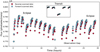 |
Fig. 1 Raw observed phase curve of WASP-18b before removal of systematics and stellar variation. The transit is shown in the inset. The observations cover two eclipses to establish a baseline; there is one transit in the middle of the observations. There is an additional half-orbit gap in the observations at 20 h due to a gyro bias update. Clear orbit-long systematics can be seen, as well as a visit-long slope, on top of the phase-curve variation. The two colours signify the exposures taken from each of the two spatial scan directions, where there is an offset due to the fixed read-out pattern of the detector. |
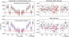 |
Fig. 2 Effect of systematic, long-term slope model on extracted phase curve. Left panels: systematics corrected phase curve and best-fit model for the wavelength bin 1.27–1.30 μm. Right panels: the same residuals plotted in time. The red line indicates the mean of the nightside residuals. In both panels, the exposures used to calculate the nightside residuals are outlined in red. Using a linear visit-long systematics model degrades the precision of the light curve, introduces visible systematics in the residuals, and results in a significant negative nightside flux. |
2.3 Estimation of errors
In order to estimate the errors on our fitted parameters and identify the degeneracies in the model we use a Markov-chain Monte Carlo approach using the open-source emcee code (Foreman-Mackey 2013). Each of the parameters are given flat priors within an acceptable range. We test the inter- and intra-chain convergence by employing the Gelmaan-Rubin diagnostic for each of our runs. We run chains of 2000 steps with 50 walkers to achieve convergence over all parameters.
3 Results
3.1 Observed phase-curve properties
The extracted white-light phase curve shows a large day-to-night contrast; this curve has a peak at 964 ± 25 ppm just before secondary eclipse and aminimum <32 ppm at 3σ level of confidence just before the primary transit (see Fig. 3). We find that day-night contrast is >0.96 in luminosity, defined in this work as the difference between the dayside and nightside phase-curve amplitude divided by the dayside amplitude. The peak of the phase curve comes before the secondary eclipse with a 4.5 ± 0.5° offset of the brightest point eastward in phase. We fit a blackbody for the planet to the dayside spectrum obtained with HST/WFC3, and find a dayside temperatureof 2894 ± 30 K. We place an upper limit on the nightside temperature of 1430 K at the 3σ level. For the spectrum of the star, we use the ATLAS9 model atmospheres grid (Castelli & Kurucz 2004), propagating uncertainty on the stellar effective temperature and planet-star radius ratio, taken from Hellier et al. (2009). These uncertainties on the system parameters correspond to a systematic uncertainty of 25 K on the planet temperature.
These results are consistent with previous phase curves of WASP-18b by Maxted et al. (2013) using Spitzer photometry at 3.6 and 4.5 μm. These authors find no evidence of a brightness offset at a 1σ precision of 5 and 9° in their respective channels, and they are unable to detect the nightside of the planet.
We extract the emission spectrum of the planet at different orbital phases (show in Fig. 4). We find that the phase-resolved spectra do not exhibit identifiable molecular features of water expected at these wavelengths. The spectra closely resemble blackbody emission at all phases and have decreasing temperature away from the secondary eclipse as expected for a tidally locked planet. This is likely explained by the dayside flux, as measured by Arcangeli et al. (2018), which dominates the emission spectrum at all phases because of the large day-night luminosity contrast (see also Parmentier et al. 2018, Fig. 10).
We additionally measure the offset of the brightest point in the phase curve in each of our 14 wavelength bins (shown in Table 1) and find that the offset remains constant with wavelength within our uncertainties. We therefore combined the measured offset from each wavelength bin to calculate a white-light curve offset of 4.5 ± 0.5° eastward in longitude. These brightness offsets are not directly equivalent to hot-spot offsets in the thermal map of the planet, as they measure theoffset in integrated hemispheric brightness (Cowan & Agol 2008; Schwartz et al. 2017). In future discussions we only compare to the brightness offset seen in our data, as the inversion from the light curve to a longitudinal brightness map is not unique.
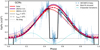 |
Fig. 3 Systematics-corrected HST/WFC3 white-light phase curve of WASP-18b (blue points) compared to suite of GCMs (coloured curves). In black is the best-fit model used to parametrise the planet signal, with two sinusoidal components for the phase-curve variation. In cyan are the stellar ellipsoidal variations, that have been subtracted from the phase curve (see Sect. 3.2). GCMs shown are parametrised by 3 drag timescales indicated by line-styles and by 3 metallicities indicated by colours (−0.5, 0.0, and +0.5 relative to solar). |
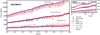 |
Fig. 4 HST/WFC3 phase-resolved spectra at three different phases (dayside, nightside, and quadratures) compared to range of GCMs. Spitzer points are taken from the best-fit sinusoidal phase-curve model by Maxted et al. (2013), where the nightside was fixed to zero flux, with error bars taken from their eclipse depth measurements. The phase bins shown are three broad bins: “Dayside” refers to orbits between phases 0.4–0.45 and 0.55–0.6, “Quadrature” to the average of phases 0.25–0.3 and 0.7–0.75, and ”Nightside” to phases 0.05–0.25 and 0.75–0.95. The same binning is used for the GCM spectra shown. |
Measured brightness offsets for each spectroscopic phase curve.
3.2 Ellipsoidal variations
We exploredthe effects of tidal deformation of the star by the planet and of the planet by the star. Since the mass of the planet is large at 10 MJup, and the planet is only separated by 3.6 stellar radii from the star, both can have a significant impact on the observed phase curve.
We use the equations supplied in Leconte et al. (2011a) and estimate that the stellar ellipsoidal variations are of order 200 or 400 ppm peak to peak. The size of these variations is uncertain owing to the uncertainty on the stellar density distribution. Since the ellipsoidal variations operate on the same timescale as our phase-curve model, they are a significant source of degeneracy. We include the magnitude of the ellipsoidal variations in our fits and remove them from our final light curves. The fitted magnitude of the stellar ellipsoidal variation is 201 ± 26 ppm in the white-light curve; a phase offset is fixed such that the minima are at secondary eclipse and transit (shown as the cyan curve in Fig. 3). We fixed the magnitude of the ellipsoidal variations to the white-light curve valuesin each of the spectroscopic phase curves.
Interestingly, our measurement of the stellar ellipsoidal variation is consistent with the independentmeasurement of the ellipsoidal variations by Shporer et al. (2019) to within the 1σ confidence level. Shporer et al. (2019) measured the amplitude of the ellipsoidal variations as 194 ± 7 ppm using observations from the TESS spacecraft in the optical. Additionally the dayside emission of WASP-18b measured with TESS is consistent with our dayside emission spectrum, as discussed in Shporer et al. (2019). However, while the planetary emission at other phases is consistent within the error bars of Shporer et al. (2019) and this work, the differences in how the planetary signal is extracted make a comparison difficult. For instance the nightside flux in TESS is measured at −24 ppm, whereas our approach enforces that the nightside signal is non-negative. We do not fix our ellipsoidal variations to the more precise measurement from Shporer et al. (2019) in order to allow us to compare the two results as independent measurements. We do however test our analysis using their value of EC = 194 ± 7 ppm and find our conclusions unchanged. The most significant effect of including their more precise measurement is an increased precision on the phase curve at quadrature, where the ellipsoidal variations peak.
We estimate the inverse effect, the tidal deformation of the planet by the star, using the tables supplied in Leconte et al. (2011b) for a 10 MJ planet under high irradiation. We find that the expected size of the variations of the planet are only an effective 0.25% in radius, equivalent to 5 ppm in the final light curve, which should be negligible at our precision and is well within the errors on the measured radius of the planet of ±6% (Southworth et al. 2009). We also estimate the effect of Doppler boosting due to the radial velocity of the star on these light curves to be about 22 ppm (Mazeh & Faigler 2010), and include this in our models fixed to this value. This is also consistent with the measurement of 24 ± 6 ppm by Shporer et al. (2019).
An additional effect of the ellipsoidal variations is that they may offset any measurements of the transit or eclipse depths when unaccounted for (e.g. Cowan et al. 2012). This effect is mitigated in the case of WASP-18b, as the phase-curve variation of the planet within the HST/WFC3 bandpass is by coincidence nearly equal in magnitude to the ellipsoidal variations over the duration of the eclipse. We estimate the difference in the retrieved eclipse depths, when the phase-curve and ellipsoidal variations are fixed to our best-fit values versus when they are unaccounted for, and modelled as instrument systematics. When these effects are not accounted for, we find a relative change in eclipse depth of only 3 ppm over the whole spectrum, well below the precision of the data, and a systematic overestimate of the eclipse depths (offset) of about 20 ppm or ~2% of the depth. These changes are within the 1-sigma errors of Arcangeli + 2018. However, we stress that for other planets where these effects do not necessarily cancel, it has been shown that their treatment can significantly affect inferred eclipse depths (Cowan et al. 2012; Kreidberg et al. 2018).
4 Comparing the phase curve of WASP-18b to global circulation models
4.1 Global circulation models
To interpret our data and determine the physical origin of the observed signals, we compare the extracted phase curve and spectra to 3D GCMs. We produced a sample of circulation models, exploring the effects of changing drag and metallicity as these have been shown to determine the broad behaviour of hot Jupiter phase curves (Showman & Polvani 2011; Kataria et al. 2015). In this workdrag refers to any dissipative mechanism that can act to slow down wave propagation and reduce windspeeds.
The atmospheric circulation and thermal structure were simulated using the SPARC/MITgcm model (Showman et al. 2009). The model solves the primitive equations in spherical geometry using the MITgcm (Adcroft et al. 2004) and the radiative transfer equations using a current 1D radiative transfer model (Marley & McKay 1999). We use the correlated-k framework to generate opacities based on the line-by-line opacities described in Visscher et al. (2006) and Freedman et al. (2014). Our initial model assumes a solar composition with elemental abundances of Lodders & Fegley (2002) and the chemical equilibrium gas-phase composition from Visscher et al. (2006). These calculations take into account the presence of H− opacities and the effect of molecular dissociation on the abundances, shown to be important for this class of planet (Arcangeli et al. 2018; Kreidberg et al. 2018; Mansfield et al. 2018; Parmentier et al. 2018; Bell & Cowan 2018). Additional heat transport by H2 recombination is not included in our models (Bell & Cowan 2018). We used a timestep of 25s, ran the simulations for 300 Earth days, averaging all quantities over the last 100 days. The above modelling process is the same as that described in Parmentier et al. (2018), using the WASP-18 system parameters from Southworth et al. (2009).
We include additional sources of drag through a Rayleigh-drag parametrisation with a single constant timescale per model that determines the efficiency with which the flow is damped. We vary this timescale between models from tdrag = 103−6s (efficient drag) and a no drag model with tdrag = ∞. While all the models are radiatively dominated on the dayside, our range of drag strengths cover the transition from a drag-free, wind circulation case to a drag-dominated circulation. This can be seen from the short radiative timescale of the dayside photospheres of our models, trad ~ 102−3s, estimated using Eq. (10) from Showman & Guillot (2002) for a simple H2 slab atmosphere. This is significantly shorter than other relevant timescales, such as the advective timescale at the equator, calculated as the ratio of the equatorial windspeed over the planet radius. The advective timescale is of the order of 104 s in our no drag model rising to 106s in our efficient drag model (tdrag = 103s), as the model atmospheres transition to drag-dominated circulations.
4.2 Comparison of GCMs to data
To first order, all of our GCMs show a large day-night contrast and small or no brightness offset, and broadly reproduce the observed phase curve of WASP-18b. We find however that our baseline, solar-composition model with no additional drag sources fails to match the size of the day-night contrast in the phase-curve data (Fig. 3). This baseline model both under-predicts the dayside flux and over-predicts the nightside flux of the planet. However, models with additional sources of drag, parametrised by a short drag timescale, are able to match better the dayside and nightside flux of the planet. All of our efficient drag models match well the day-night contrast of the planet. We therefore find that we require additional drag sources to explain our observed day-night contrast of WASP-18b. We discuss the possible physical origins of this additional drag in Sect. 5.1.
When generating our GCMs, we held the system parameters fixed to literature values. We were not able to explore their full uncertainties as generating one model is already computationally expensive. However, uncertainties on the system parameters lead to an additional uncertainties on the inferred best-fit models. Since the differences between the efficient drag models are so small, we cannot statistically choose between these models (see Table 2). Nevertheless, models with inefficient or no drag fail to reproduce the day-night contrast seen in the data and therefore the overall shape of the phase curve. Hence we can conclude that we require some additional source of efficient drag to explain our observed phase curve, and the best-fitting models are those with tdrag = 103 or 104 s.
We test whether enhanced or depleted metallicity might also explain the large day-night contrast without the need for additional drag sources (Kataria et al. 2015). We find however that the effect of changing metallicity alone, in our models of WASP-18b, is too small to explain the observations (see Fig. 3), but the effect of metallicity on the phase curve is different for these hot planets compared too cooler objects (see Sect. 5.3).
We also compare our GCMs to phase-resolved spectra extracted from the spectroscopic phase curve, as this allows us to study the wavelength dependence of our data. As seen in Fig. 4, we find that the spectra are best matched by the efficient drag models. The phase-resolved spectra are dominated by thermal emission from the dayside owing to the large day-night luminosity contrast.
Fit quality between our circulation models and the measured phase curve of WASP-18b, relative to the best-fitting model.
5 Discussion
5.1 Dragin global circulation models
5.1.1 Sources of drag
We infer thepresence of an efficient drag source in the atmosphere of WASP-18b from our comparison to GCMs. We explore the origins of this drag, which could originate from a variety of sources, such as turbulence and instabilities (Goodman 2009; Li & Goodman 2010; Youdin & Mitchell 2010), or hydrodynamic shocks (Dobbs-Dixon et al. 2010; Rauscher & Menou 2010; Heng 2012; Fromang et al. 2016). Alternatively, for hot planets whose atmospheres are partially ionised, magnetic fields may influence the circulation and create a magnetic drag (Perna et al. 2010a; Batygin et al. 2013; Komacek et al. 2017). Magnetic drag, sometimes called “ion drag”, is caused by the collision between the bulk neutral flow and the ionic component of the flow. Since the ionic component is subject to Lorentz forces but the neutral component is not, these ions can act as a drag and eventually dominate the circulation under the right conditions (Zhu et al. 2005).
Alkali metals in the dayside atmosphere of WASP-18b should be significantly thermally ionised (Arcangeli et al. 2018; Helling et al. 2019). Thus, if WASP-18b were to host a magnetic field, its circulation would be influenced by magnetic drag. We use the formula described in Perna et al. 2010a (here Eq. (2)) to estimate what might be the efficiency of magnetic drag on this planet, parametrised through the timescale tdrag,
 (2)
(2)
This timescale tdrag is the timescale on which kinetic energy is dissipated by magnetic drag in the atmosphere. We calculated the ionisation fraction in local chemical equilibrium for our circulation models with a modified version of the NASA CEA Gibbs minimisation code (e.g. Gordon & McBride 1994; Parmentier et al. 2018). This ionisation fraction (ne) is used to compute η, the resistivity, defined in Perna et al. (2010a). The value B is the magnetic field strength, ρ is the density of the atmosphere, and π − θ is the angle between the magnetic field and the flow (assumed that θ = 0 for the case of maximal efficiency).
We find that we can match a tdrag of order 103 s at the substellar point, rising to 104 s elsewhere on the dayside, with a magnetic field strength of B = 10 gauss. The nightside drag timescale from our models is much longer, as the nightside is too cold for thermal ionisation. This estimate shows that the short drag timescale inferred from our GCMs could reasonably be due to Lorentz forces. However, the inhomogeneity also highlights that our Rayleigh-drag parametrisation does not capture the full effects of magnetic drag, as for instance a magnetic drag timescale should vary throughout the atmosphere.
5.1.2 Limitations of Rayleigh drag parametrisation
In our GCMs, drag is parametrised by a simple Rayleigh drag (Komacek & Showman 2016) which aims to approximate any additional drag sources by one single dissipative timescale throughout the planet, without the need for finer resolutions or full magneto-hydrodynamic calculations. This parametrisation is shown in Eq. (3), where the drag force per unit mass,  , is given as v, the velocity of the flow, divided by tdrag, a single constant drag timescale, i.e.
 (3)
(3)
In the context of magnetic drag, this parametrisation has three key problems. The first is that the magnetic drag is direction-dependent with respect to the magnetic field (Batygin et al. 2013) seen as the θ term in Eq. (2). The second is that the strength of drag is spatially inhomogeneous, i.e. it is weaker in cooler regions where there is less ionisation, such as the nightside hemisphere (Rauscher & Menou 2012). Finally, the atmospheric circulation itself can induce a toroidal magnetic field that is larger in amplitude than the dipole field of the planet, which can change both the strength and direction of the Lorentz force (Rogers & Komacek 2014). All these aforementioned effects are not accounted for in our models which could limit our accuracy in predicting the shape of the phase curve.
5.2 Effect of a planetary magnetic field
5.2.1 Magnetic circulation
Batygin et al. (2013) further explored the effect of the directionally-dependent Lorentz-force on atmospheric circulation. Our GCMs with very efficient drag exhibit longitudinally symmetric day-night flow patterns (top panel of Fig. 5), as efficient drag shuts down Rossby and Kelvin waves in the dayside atmosphere that are responsible for the typical equatorial jet formation (Showman & Polvani 2011). However Batygin et al. (2013) suggested that this should only occur on objects with low magnetic fields, typically with B < 0.5 gauss in strength. These authors predicted that the majority of highly irradiated gas giant atmospheres should be dominated by zonal jets (Showman & Polvani 2011), such as those seen in our drag free models (bottom panel of Fig. 5). This is due to Lorentz forces that act perpendicular to the magnetic field lines leading to circulation patterns with zonal jets, rather than simply damping the existing flow as in the Rayleignash-drag parametrisation (Batygin et al. 2013). In contrast, without considering magnetic effects, drag due to other schemes such as the Kelvin–Helmholtz instability should lead to a symmetric day-night flow with no brightness offset. In this context, the presence of a brightness offset in our data might be an indication that magnetic effects are responsible for the observed circulation on WASP-18b, and therefore favour a magnetic drag scenario.
Magnetic drag should affect the circulation of cooler planets more than UHJs. As discussed in Perna et al. (2010a) for HD 209458b (Teq = 1460 K), magnetic drag may act to limit the wind speeds, but does not completely shut down recirculation for magnetic fields with B < 30 gauss or so. This is because there is a direct dependence of the magnetic drag timescale on the resistivity of the atmosphere (see Eq. (2)). This resistivity depends strongly on the local temperature through the ionisation fraction, which drops sharply even across the dayside of WASP-18b (see Helling et al. 2019, Fig. 6).
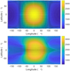 |
Fig. 5 Temperature and wind maps of WASP-18b taken from GCMs at a pressure level of 0.2 bar for two cases of drag. Top: efficient dragmodel (tdrag = 103 s) shows the circulation is day-to-night and longitudinally symmetric. Bottom: no drag model shows the circulation to the nightside is more efficient and driven by an equatorial jet. |
5.2.2 Ohmic dissipation in WASP-18b
Another consequence of a planetary magnetic field is Ohmic dissipation which has been proposed as a mechanism to explain hot Jupiter inflation (Batygin & Stevenson 2010; Perna et al. 2010b; Menou 2012). Here we consider what the effect of Ohmic dissipation would be on the measured radius of WASP-18b.
In the specific case of WASP-18b, there are two additional factors affecting the radius inflation by Ohmic dissipation because of its high temperature and high mass. The first is that heating due to Ohmic dissipation should be less efficient in the presence of efficient drag, as the zonal winds that drive Ohmic dissipation are reduced in speed (Menou 2012). The second is that inflation by Ohmic dissipation should be less efficient for higher mass planets (Huang & Cumming 2012). This is because the depth at which Ohmic power is deposited depends on the scale height of the atmosphere, and energy should be deposited higher in massive planet atmospheres than less massive planets. This would reduce the effect of any additional heating by Ohmic dissipation on the observed radius of massive planets.
These effects combined predict that WASP-18b should not be significantly inflated by Ohmic dissipation. Using predictions from Thorngren & Fortney (2018), a 10 MJ planet should have a maximum radius of 1.21 RJ when inflation effects are not taken into account. The measured radius of WASP-18b is consistent with this value within one sigma (1.204 ± 0.035; Maxted et al. 2013). The effect of inflation on the radius of high mass planets is harder to detect (Miller et al. 2009), however we can conclude that WASP-18b does not deviate from the scenario predicted by Ohmic dissipation. In Sect. 5.5, we show that we can lift some of this degeneracy between mass and inflation efficiency by comparing to a lower mass UHJ, i.e. WASP-103b.
5.3 Effect of atmospheric metallicity on the phase curve of WASP-18b
Previous work has shown that changes in atmospheric metallicity can affect global circulation in hot Jupiter atmospheres (Showman et al. 2009; Kataria et al. 2015). For instance, increasing the metallicity in a classical hot Jupiter model typically acts to reduce the nightside emission of a planet (e.g. WASP-43b, Kataria et al. 2015). This is because, as the metallicity increases, the abundances of molecular species increase leading to stellar light being absorbed higher in the atmosphere, at lower pressures. The radiative timescale is shorter at lower pressures, leading to less efficient heat circulation to the nightside of the planet (Showman et al. 2009). Additionally, as more incident energy is re-irradiated from the dayside, the brightness temperature of the dayside increases with increasing metallicity for a classical hot Jupiter model (Kataria et al. 2015).
WASP-18b resides in a hotter regime, where for instance gas-phase TiO becomes an important chemical species. For WASP-18b, an increase in atmospheric metallicity changes the abundance ratio of gas-phase TiO versus H2 O above the photosphere (Parmentier et al. 2018). While TiO absorption increases the temperature above the band-averaged WFC3 photosphere, the temperature at the WFC3 photosphere decreases, as correspondingly less stellar light reaches photospheric pressures. Hence the dayside of the planet is dimmer in the WFC3 bandpass in the higher metallicity case, but should be brighter in emission shorter than 1 μm, inside the TiO bandpass. The reverse effect is seen when the metallicity is decreased. The temperature of the WFC3 photosphere is hotter but the nightside re-circulation is more efficient, leading to an increase in emission at all phases in the WFC3 bandpass.
Neither an enhancement or depletion of ±0.5 in metallicity relative to solar is sufficient to match the observed phase curve of WASP-18b without including efficient drag in our models. However, there is a strong dependence of the nightside temperature with metallicity in our no-drag models (see Figs. 3 and 4).
5.4 Constraints on the redistribution
The redistribution efficiency determines the amount of flux that is re-emitted from the dayside versus the amount of flux that is carried to the nightside. It can be defined through the ratio of the dayside temperature and equilibrium temperature of the planet:  . In this case f = 2 refers to the dayside-only redistribution case, while f = 2.67 refers to theno-redistribution case (where the dayside reaches the maximum temperature). The redistribution efficiency can be used as a simple measure of the atmospheric circulation regime. We show the redistribution efficiencies for each of our GCMs in Fig. 6 as the coloured points. All of our GCMs have redistribution factors between 2.2 < f < 2.5.
These models for WASP-18b show that the redistribution efficiency is strongly dependent on metallicity in the case of no or weak drag. This can be seen as the steep dependence of redistribution efficiency with metallicity for the left-most points in Fig. 6 (the weak drag regime). The origin of this effect is described in Sect. 5.3. For models with efficient drag, the dependence of redistribution on metallicity is greatly reduced. In these models the circulation becomes drag dominated and inefficient at all pressures, hence the effect of metallicity is less pronounced.
Typically the redistribution efficiency cannot be estimated solely from the dayside emission, as there is a known degeneracy between the albedo and redistribution efficiency (Cowan & Agol 2011). For UHJs, while the albedos are expected to be very small, we illustrate that the uncertainty on the equilibrium temperature limits any conclusions that could be drawn from the dayside alone. The redistribution efficiencies calculated in Arcangeli et al. (2018) adopted fixed stellar parameters during the retrieval process, fixing Teq = 2477 K. This is offset from our GCMs, calculated using slightly different stellar parameters, leading to Teq = 2385 K. We correct for this offset and include a systematic uncertainty of Δf = ±0.18 from ΔTeq = ±44 K (Southworth et al. 2009). In Fig. 6, we plot these modified metallicity/redistribution contours from Arcangeli et al. (2018). We see that the uncertainty on Teq dominates over the retrieved errors and needs to be included when retrieving the redistribution from the dayside alone.
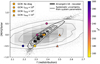 |
Fig. 6 Metallicity as a function of redistribution efficiency, comparing 1D modelling to our 3D GCMs. The GCM outputs are shown by coloured markers, where marker styles indicate the drag strength in each model: from right to left tdrag = 103s (triangles), 104s (squares), 106 s (hexagon), and no-drag (circles). Markers are also coloured by χ2 between the corresponding GCM phase curve and our HST/WFC3 phase curve. Retrieved redistribution efficiencies from Arcangeli et al. (2018) are shown by black contours; the same contours, including a systematic uncertainty on the equilibrium temperature of 44 K, are shown in grey. |
5.5 Comparison of two ultra hot Jupiters
Spectroscopic phase curves with HST/WFC3 have been published for three exoplanets so far, WASP-43b (Stevenson et al. 2014), WASP-103b (Kreidberg et al. 2018), and WASP-18 (this work). Of these planets, WASP-18b and WASP-103b both belong to the class of UHJs, while WASP-43b is in a cooler regime (Teq = 1370 K). The inferred properties, spectra, and phase curves of these two UHJs have many similarities (see Table 3). However, key differences between these planets remain, namely their masses, radius anomalies, and measured brightness offsets.
The differences between these two planets can shed further light on their atmospheric properties. A first major difference is in their observed circulations: WASP-18b has a small but significant phase-curve offset, whereas the phase curve of WASP-103b appears longitudinally symmetric. In the simple picture of circulation as a balance of the radiative and advective timescales (Showman & Guillot 2002), we would expect the day-night contrast of WASP-18b to be lower than WASP-103b, as the brightness offset should correspond to moderately efficient wind-driven circulation. However the observed day-night contrast of WASP-18b is larger than WASP-103b, in conflict with this simple picture. As suggested in Sect. 5.1, the observed offset of WASP-18b may be the result of a magnetic field, and an offset may not be present on WASP-103bif the planet were to host a weaker magnetic field, as might be expected from its lower mass (Yadav & Thorngren 2017).
The second major difference is that WASP-103b is very inflated, while WASP-18b is consistent with a non-inflated model (see Sect. 5.2.2). The radius of WASP-103b should be about 1.10 RJup when no inflation mechanism is present (Thorngren & Fortney 2018). From the results of Miller et al. (2009), an additional constant heat source of 1029 erg s−1 could explain the inflated radius of WASP-103b. For this same additional heating, an inflated WASP-18b would have a radius of 1.3 RJup (Miller et al. 2009). This is marginally larger than the observed radius of WASP-18b by 2σ. Thus WASP-18b appears slightly less inflated than WASP-103b despite being around an almost identical star and at the same dayside temperature. One inflation mechanism that can explain this difference is Ohmic dissipation as, for a fixed additional heating, it is less efficient and inflates the radii of a higher mass planet (Huang & Cumming 2012).
These two differences both highlight that there is a greater complexity behind the observed properties, such as the phase-curve properties, in particular in the role that magnetic fields might play on the circulation or radius inflation. Importantly, we can use planets such as UHJs as a test for inflation theories, as they occupy a parameter space where inflation models differ (Sestovic et al. 2018; Thorngren & Fortney 2018).
Comparison of measured and inferred properties of the WASP-18 and WASP-103 UHJ systems.
6 Conclusions
We observed one full orbit phase curve of the UHJ WASP-18b. We find the peak signal from the dayside at an effective temperature of 2894 ± 30 K and do not detect the nightside of the planet, placing an upper limit of 1430K at 3σ. We find a large day-night-contrast of >0.96 in luminosity and a small offset of the brightest point from the substellar point by 4.5 ± 0.5°.
We compare the extracted spectroscopic phase curve with GCM and find that the data can be best reproduced by models with efficient drag. Models without additional drag sources fail to reproduce the day-night contrast seen in our data, hence we require an additional drag source to explain the observed day-night contrast. We also find that the behaviour of the phase curve of WASP-18b with metallicity is different from cooler planets, owing to the high temperature chemistry of TiO and water in the atmosphere of WASP-18b. In addition to this, we show that a metallicity enhancement or depletion in our models is not sufficient to match the observed day-night contrast without the presence of efficient drag.
We explore the origin of this efficient drag, and show that it could be due to Lorentz forces on ionised metals in the atmosphere from a magnetic field as weak as 10 gauss. The effect of a magnetic field on the circulation may also explain the small brightness offset seen in our data, however our models do not explore the full dependence of the circulation on magnetic effects, which will require further studies.
Furthermore, we compare our results to the recently published phase curve of WASP-103b (Kreidberg et al. 2018). We find that the two planets are consistent with the expectation that more massive planets should be less inflated, and support the theory of Ohmic dissipation as an inflation mechanism. However, their different circulations point to a more complicated picture and suggest that other fundamental properties of these systems, such as their magnetic fields, may be different.
Acknowledgements
We thank N. Cowan for a thorough referee report that greatly improved the clarity of this work. We also thank D. Thorngren for providing tables of predicted planet radii used in this work, and we thank C. Helling for many fruitful discussions. J.M.D. acknowledges that the research leading to these results has received funding from the European Research Council (ERC) under the European Union’s Horizon 2020 research and innovation programme (grant agreement no. 679633; Exo-Atmos). J.M.D acknowledges support by the Amsterdam Academic Alliance (AAA) Program. Support for program GO-13467 was provided to the US-based researchers by NASA through a grant from the Space Telescope Science Institute, which is operated by the Association of Universities for Research in Astronomy, Inc., under NASA contract NAS 5-26555. J.L.B. acknowledges support from the David and Lucile Packard Foundation.
Appendix A Additional material
Best-fit values resulting from the white-light curve fit.
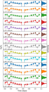 |
Fig. A.1 Extracted spectroscopic phase curves shown with histograms of residuals. Solid curves indicate fits to the data. |
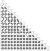 |
Fig. A.2 Corner plot of posteriors for the white-light curve fit. Result of 10 000 steps per 50 walkers. Generated using corner.py (Foreman-Mackey 2016). Histogram titles show means and ± 1σ confidence intervals of the samples. |
References
- Adcroft, A., Campin, J.-M., Hill, C., & Marshall, J. 2004, Mon. Weather Rev., 132, 2845 [NASA ADS] [CrossRef] [Google Scholar]
- Arcangeli, J., Désert, J.-M., Line, M. R., et al. 2018, ApJ, 855, L30 [NASA ADS] [CrossRef] [Google Scholar]
- Armstrong, D. J., de Mooij, E., Barstow, J., et al. 2016, Nat. Astron., 1, 0004 [NASA ADS] [CrossRef] [Google Scholar]
- Batygin, K., & Stevenson, D. J. 2010, ApJ, 714, L238 [NASA ADS] [CrossRef] [Google Scholar]
- Batygin, K., Stanley, S., & Stevenson, D. J. 2013, ApJ, 776, 53 [NASA ADS] [CrossRef] [Google Scholar]
- Bell, T. J., & Cowan, N.b. 2018, ApJ, 857, L20 [NASA ADS] [CrossRef] [Google Scholar]
- Bell, T. J., Nikolov, N., Cowan, N. B., et al. 2017, ApJ, 847, L2 [NASA ADS] [CrossRef] [Google Scholar]
- Borucki, W. J., Koch, D., Jenkins, J., et al. 2009, Science, 325, 709 [NASA ADS] [CrossRef] [PubMed] [Google Scholar]
- Castelli, F., & Kurucz, R. L. 2004, IAU Symp., 210, A20 [Google Scholar]
- Charbonneau, D., Allen, L. E., Megeath, S. T., et al. 2005, ApJ, 626, 523 [NASA ADS] [CrossRef] [Google Scholar]
- Cowan, N. B., & Agol, E. 2008, ApJ, 678, L129 [NASA ADS] [CrossRef] [Google Scholar]
- Cowan, N. B., & Agol, E. 2011, ApJ, 729, 54 [NASA ADS] [CrossRef] [Google Scholar]
- Cowan, N. B., Agol, E., & Charbonneau, D. 2007, MNRAS, 379, 641 [NASA ADS] [CrossRef] [Google Scholar]
- Cowan, N. B., Machalek, P., Croll, B., et al. 2012, ApJ, 747, 82 [NASA ADS] [CrossRef] [Google Scholar]
- Dang, L., Cowan, N.b., Schwartz, J. C., et al. 2018, Nat. Astron., 2, 220 [NASA ADS] [CrossRef] [Google Scholar]
- Deming, D., Brown, T. M., Charbonneau, D., Harrington, J., & Richardson, L. J. 2005, ApJ, 622, 1149 [NASA ADS] [CrossRef] [Google Scholar]
- Désert, J.-M., Charbonneau, D., Fortney, J. J., et al. 2011a, ApJS, 197, 11 [NASA ADS] [CrossRef] [Google Scholar]
- Désert, J.-M., Charbonneau, D., Demory, B.-O., et al. 2011b, ApJS, 197, 14 [NASA ADS] [CrossRef] [Google Scholar]
- Dobbs-Dixon, I., Cumming, A., & Lin, D. N. C. 2010, ApJ, 710, 1395 [NASA ADS] [CrossRef] [Google Scholar]
- Feng, Y. K., Line, M. R., Fortney, J. J., et al. 2016, ApJ, 829, 52 [NASA ADS] [CrossRef] [Google Scholar]
- Foreman-Mackey, D. 2016, J. Open Source Softw., 1, 24 [Google Scholar]
- Foreman-Mackey, D., Hogg, D. W., Lang, D., & Goodman, J. 2013, PASP, 125, 306 [CrossRef] [Google Scholar]
- Freedman, R. S., Lustig-Yaeger, J., Fortney, J. J., et al. 2014, ApJS, 214, 25 [NASA ADS] [CrossRef] [Google Scholar]
- Fromang, S., Leconte, J., & Heng, K. 2016, A&A, 591, A144 [NASA ADS] [CrossRef] [EDP Sciences] [Google Scholar]
- Goodman, J. 2009, ApJ, 693, 1645 [NASA ADS] [CrossRef] [Google Scholar]
- Gordon, S., & McBride, B. J. 1994, Computer Program for Calculation of Complex Chemical Equilibrium Compositions and Applications. I. Analysis (Washington, DC: NASA) [Google Scholar]
- Haynes, K., Mandell, A. M., Madhusudhan, N., Deming, D., & Knutson, H. 2015, ApJ, 806, 146 [NASA ADS] [CrossRef] [Google Scholar]
- Hellier, C., Anderson, D. R., Collier Cameron, A., et al. 2009, Nature, 460, 1098 [NASA ADS] [CrossRef] [Google Scholar]
- Helling, C., Gourbin, P., Woitke, P., & Parmentier, V. 2019, A&A, in press, DOI: 10.1051/0004-6361/201834085 [Google Scholar]
- Heng, K. 2012, ApJ, 761, L1 [NASA ADS] [CrossRef] [Google Scholar]
- Hindle, A. W., Bushby, P. J., & Rogers, T. M. 2019, ApJ, 872, L27 [NASA ADS] [CrossRef] [Google Scholar]
- Huang, X., & Cumming, A. 2012, ApJ, 757, 47 [NASA ADS] [CrossRef] [Google Scholar]
- Iro, N., & Maxted, P. F. L. 2013, Icarus, 226, 1719 [NASA ADS] [CrossRef] [Google Scholar]
- Kataria, T., Showman, A. P., Fortney, J. J., et al. 2015, ApJ, 801, 86 [NASA ADS] [CrossRef] [Google Scholar]
- Kataria, T., Sing, D. K., Lewis, N. K., et al. 2016, ApJ, 821, 9 [NASA ADS] [CrossRef] [Google Scholar]
- Keating, D., & Cowan, N.b. 2017, ApJ, 849, L5 [Google Scholar]
- Keating, D., & Cowan, N. B. 2018, ArXiv e-prints [arXiv:1809.00002] [Google Scholar]
- Kitzmann, D., Heng, K., Rimmer, P. B., et al. 2018, ApJ, 863, 183 [NASA ADS] [CrossRef] [Google Scholar]
- Knutson, H. A., Charbonneau, D., Allen, L. E., et al. 2007, Nature, 447, 183 [NASA ADS] [CrossRef] [PubMed] [Google Scholar]
- Knutson, H. A., Lewis, N., Fortney, J. J., et al. 2012, ApJ, 754, 22 [NASA ADS] [CrossRef] [Google Scholar]
- Komacek, T. D., & Showman, A. P. 2016, ApJ, 821, 16 [NASA ADS] [CrossRef] [Google Scholar]
- Komacek, T. D., Showman, A. P., & Tan, X. 2017, ApJ, 835, 198 [NASA ADS] [CrossRef] [Google Scholar]
- Kreidberg, L. 2015, PASP, 127, 1161 [NASA ADS] [CrossRef] [Google Scholar]
- Kreidberg, L., Bean, J. L., Désert, J.-M., et al. 2014, Nature, 505, 69 [NASA ADS] [CrossRef] [Google Scholar]
- Kreidberg, L., Line, M. R., Parmentier, V., et al. 2018, AJ, 156, 17 [NASA ADS] [CrossRef] [Google Scholar]
- Leconte, J., Lai, D., & Chabrier, G. 2011a, A&A, 536, C1 [NASA ADS] [CrossRef] [EDP Sciences] [Google Scholar]
- Leconte, J., Lai, D., & Chabrier, G. 2011b, A&A, 528, A41 [NASA ADS] [CrossRef] [EDP Sciences] [Google Scholar]
- Li, J., & Goodman, J. 2010, ApJ, 725, 1146 [NASA ADS] [CrossRef] [Google Scholar]
- Line, M. R., & Parmentier, V. 2016, ApJ, 820, 78 [NASA ADS] [CrossRef] [Google Scholar]
- Lothringer, J. D., Barman, T., & Koskinen, T. 2018, ApJ, 866, 27 [NASA ADS] [CrossRef] [Google Scholar]
- Lodders, K., & Fegley, B. 2002, Icarus, 155, 393 [NASA ADS] [CrossRef] [Google Scholar]
- Lodders, K., Palme, H., & Gail, H.-P. 2009, Landolt Börnstein (Berlin: Springer-Verlag) [Google Scholar]
- Mansfield, M., Bean, J. L., Line, M. R., et al. 2018, AJ, 156, 10 [NASA ADS] [CrossRef] [Google Scholar]
- Marley, M. S., & McKay, C. P. 1999, Icarus, 138, 268 [NASA ADS] [CrossRef] [Google Scholar]
- Maxted, P. F. L., Anderson, D. R., Doyle, A. P., et al. 2013, MNRAS, 428, 2645 [NASA ADS] [CrossRef] [Google Scholar]
- Mazeh, T., & Faigler, S. 2010, A&A, 521, L59 [NASA ADS] [CrossRef] [EDP Sciences] [Google Scholar]
- Menou, K. 2012, ApJ, 745, 138 [NASA ADS] [CrossRef] [Google Scholar]
- Miller, N., Fortney, J. J., & Jackson, B. 2009, ApJ, 702, 1413 [NASA ADS] [CrossRef] [Google Scholar]
- Nymeyer, S., Harrington, J., Hardy, R. A., et al. 2011, ApJ, 742, 35 [NASA ADS] [CrossRef] [Google Scholar]
- Parmentier, V., & Crossfield, I. 2018, Handbook of Exoplanets (Berlin: Springer International), 116 [Google Scholar]
- Parmentier, V., Showman, A. P., & Lian, Y. 2013, A&A, 558, A91 [NASA ADS] [CrossRef] [EDP Sciences] [Google Scholar]
- Parmentier, V., Fortney, J. J., Showman, A. P., Morley, C., & Marley, M. S. 2016, ApJ, 828, 22 [NASA ADS] [CrossRef] [Google Scholar]
- Parmentier, V., Line, M. R., Bean, J. L., et al. 2018, A&A, 617, A110 [NASA ADS] [CrossRef] [EDP Sciences] [Google Scholar]
- Pepper, J., Pogge, R. W., DePoy, D. L., et al. 2007, PASP, 119, 923 [NASA ADS] [CrossRef] [Google Scholar]
- Pepper, J., Kuhn, R. B., Siverd, R., James, D., & Stassun, K. 2012, PASP, 124, 230 [NASA ADS] [CrossRef] [Google Scholar]
- Perez-Becker, D., & Showman, A. P. 2013, ApJ, 776, 134 [NASA ADS] [CrossRef] [Google Scholar]
- Perna, R., Menou, K., & Rauscher, E. 2010a, ApJ, 719, 1421 [NASA ADS] [CrossRef] [Google Scholar]
- Perna, R., Menou, K., & Rauscher, E. 2010b, ApJ, 724, 313 [NASA ADS] [CrossRef] [Google Scholar]
- Pollacco, D. L., Skillen, I., Collier Cameron, A., et al. 2006, PASP, 118, 1407 [NASA ADS] [CrossRef] [Google Scholar]
- Rauscher, E., & Kempton, E. M. R. 2014, ApJ, 790, 79 [NASA ADS] [CrossRef] [Google Scholar]
- Rauscher, E., & Menou, K. 2010, ApJ, 714, 1334 [NASA ADS] [CrossRef] [Google Scholar]
- Rauscher, E., & Menou, K. 2012, ApJ, 745, 78 [NASA ADS] [CrossRef] [Google Scholar]
- Rogers, T. M. 2017, Nat. Astron., 1, 131 [NASA ADS] [CrossRef] [Google Scholar]
- Rogers, T. M., & Komacek, T. D. 2014, ApJ, 794, 132 [NASA ADS] [CrossRef] [Google Scholar]
- Schwartz, J. C., Kashner, Z., Jovmir, D., et al. 2017, ApJ, 850, 154 [NASA ADS] [CrossRef] [Google Scholar]
- Sestovic, M., Demory, B.-O., & Queloz, D. 2018, A&A, 616, A76 [NASA ADS] [CrossRef] [EDP Sciences] [Google Scholar]
- Sheppard, K.b., Mandell, A. M., Tamburo, P., et al. 2017, ApJ, 850, L32 [NASA ADS] [CrossRef] [Google Scholar]
- Showman, A. P., & Guillot, T. 2002, A&A, 385, 166 [NASA ADS] [CrossRef] [EDP Sciences] [Google Scholar]
- Showman, A. P., & Polvani, L. M. 2011, ApJ, 738, 71 [NASA ADS] [CrossRef] [Google Scholar]
- Showman, A. P., Fortney, J. J., Lian, Y., et al. 2009, ApJ, 699, 564 [NASA ADS] [CrossRef] [Google Scholar]
- Showman, A. P., Lewis, N. K., & Fortney, J. J. 2015, ApJ, 801, 95 [NASA ADS] [CrossRef] [Google Scholar]
- Shporer, A., Wong, I., Huang, C. X., et al. 2019, AJ, 157, 178 [NASA ADS] [CrossRef] [Google Scholar]
- Snellen, I. A. G., de Mooij, E. J. W., & Albrecht, S. 2009, Nature, 459, 543 [NASA ADS] [CrossRef] [PubMed] [Google Scholar]
- Snellen, I., Stuik, R., Otten, G., et al. 2013, Eur. Phys. J. Web Conf., 47, 03008 [CrossRef] [EDP Sciences] [Google Scholar]
- Southworth, J., Hinse, T. C., Dominik, M., et al. 2009, ApJ, 707, 167 [NASA ADS] [CrossRef] [Google Scholar]
- Southworth, J., Mancini, L., Ciceri, S., et al. 2015, MNRAS, 447, 711 [NASA ADS] [CrossRef] [Google Scholar]
- Stevenson, K.b., Désert, J.-M., Line, M. R., et al. 2014, Science, 346, 838 [NASA ADS] [CrossRef] [Google Scholar]
- Stevenson, K.b., Line, M. R., Bean, J. L., et al. 2017, AJ, 153, 68 [NASA ADS] [CrossRef] [Google Scholar]
- Thorngren, D. P., & Fortney, J. J. 2018, AJ, 155, 214 [NASA ADS] [CrossRef] [Google Scholar]
- Visscher, C., Lodders, K., & Fegley, B., Jr. 2006, ApJ, 648, 1181 [NASA ADS] [CrossRef] [Google Scholar]
- Wong, I., Knutson, H. A., Lewis, N. K., et al. 2015, ApJ, 811, 122 [NASA ADS] [CrossRef] [Google Scholar]
- Wong, I., Knutson, H. A., Kataria, T., et al. 2016, ApJ, 823, 122 [NASA ADS] [CrossRef] [Google Scholar]
- Yadav, R. K., & Thorngren, D. P. 2017, ApJ, 849, L12 [NASA ADS] [CrossRef] [Google Scholar]
- Youdin, A. N., & Mitchell, J. L. 2010, ApJ, 721, 1113 [NASA ADS] [CrossRef] [Google Scholar]
- Zhu, X., Talaat, E. R., Baker, J. B. H. & Yee, H.-H. 2005, Ann. Geo. 2005, 23, 3313 [NASA ADS] [CrossRef] [Google Scholar]
All Tables
Fit quality between our circulation models and the measured phase curve of WASP-18b, relative to the best-fitting model.
Comparison of measured and inferred properties of the WASP-18 and WASP-103 UHJ systems.
All Figures
|
Fig. 1 Raw observed phase curve of WASP-18b before removal of systematics and stellar variation. The transit is shown in the inset. The observations cover two eclipses to establish a baseline; there is one transit in the middle of the observations. There is an additional half-orbit gap in the observations at 20 h due to a gyro bias update. Clear orbit-long systematics can be seen, as well as a visit-long slope, on top of the phase-curve variation. The two colours signify the exposures taken from each of the two spatial scan directions, where there is an offset due to the fixed read-out pattern of the detector. |
| In the text | |
|
Fig. 2 Effect of systematic, long-term slope model on extracted phase curve. Left panels: systematics corrected phase curve and best-fit model for the wavelength bin 1.27–1.30 μm. Right panels: the same residuals plotted in time. The red line indicates the mean of the nightside residuals. In both panels, the exposures used to calculate the nightside residuals are outlined in red. Using a linear visit-long systematics model degrades the precision of the light curve, introduces visible systematics in the residuals, and results in a significant negative nightside flux. |
| In the text | |
|
Fig. 3 Systematics-corrected HST/WFC3 white-light phase curve of WASP-18b (blue points) compared to suite of GCMs (coloured curves). In black is the best-fit model used to parametrise the planet signal, with two sinusoidal components for the phase-curve variation. In cyan are the stellar ellipsoidal variations, that have been subtracted from the phase curve (see Sect. 3.2). GCMs shown are parametrised by 3 drag timescales indicated by line-styles and by 3 metallicities indicated by colours (−0.5, 0.0, and +0.5 relative to solar). |
| In the text | |
|
Fig. 4 HST/WFC3 phase-resolved spectra at three different phases (dayside, nightside, and quadratures) compared to range of GCMs. Spitzer points are taken from the best-fit sinusoidal phase-curve model by Maxted et al. (2013), where the nightside was fixed to zero flux, with error bars taken from their eclipse depth measurements. The phase bins shown are three broad bins: “Dayside” refers to orbits between phases 0.4–0.45 and 0.55–0.6, “Quadrature” to the average of phases 0.25–0.3 and 0.7–0.75, and ”Nightside” to phases 0.05–0.25 and 0.75–0.95. The same binning is used for the GCM spectra shown. |
| In the text | |
|
Fig. 5 Temperature and wind maps of WASP-18b taken from GCMs at a pressure level of 0.2 bar for two cases of drag. Top: efficient dragmodel (tdrag = 103 s) shows the circulation is day-to-night and longitudinally symmetric. Bottom: no drag model shows the circulation to the nightside is more efficient and driven by an equatorial jet. |
| In the text | |
|
Fig. 6 Metallicity as a function of redistribution efficiency, comparing 1D modelling to our 3D GCMs. The GCM outputs are shown by coloured markers, where marker styles indicate the drag strength in each model: from right to left tdrag = 103s (triangles), 104s (squares), 106 s (hexagon), and no-drag (circles). Markers are also coloured by χ2 between the corresponding GCM phase curve and our HST/WFC3 phase curve. Retrieved redistribution efficiencies from Arcangeli et al. (2018) are shown by black contours; the same contours, including a systematic uncertainty on the equilibrium temperature of 44 K, are shown in grey. |
| In the text | |
|
Fig. A.1 Extracted spectroscopic phase curves shown with histograms of residuals. Solid curves indicate fits to the data. |
| In the text | |
|
Fig. A.2 Corner plot of posteriors for the white-light curve fit. Result of 10 000 steps per 50 walkers. Generated using corner.py (Foreman-Mackey 2016). Histogram titles show means and ± 1σ confidence intervals of the samples. |
| In the text | |
Current usage metrics show cumulative count of Article Views (full-text article views including HTML views, PDF and ePub downloads, according to the available data) and Abstracts Views on Vision4Press platform.
Data correspond to usage on the plateform after 2015. The current usage metrics is available 48-96 hours after online publication and is updated daily on week days.
Initial download of the metrics may take a while.