| Issue |
A&A
Volume 625, May 2019
|
|
|---|---|---|
| Article Number | A16 | |
| Number of page(s) | 9 | |
| Section | Planets and planetary systems | |
| DOI | https://doi.org/10.1051/0004-6361/201834640 | |
| Published online | 01 May 2019 | |
HD 2685 b: a hot Jupiter orbiting an early F-type star detected by TESS★
1
European Southern Observatory,
Alonso de Córdova 3107, Vitacura,
Casilla
19001,
Santiago,
Chile
e-mail: This email address is being protected from spambots. You need JavaScript enabled to view it.
2
Instituto de Astrofísica, Facultad de Física, Pontificia Universidad Católica de Chile,
Av. Vicuña Mackenna 4860,
7820436
Macul,
Santiago,
Chile
3
Millennium Institute of Astrophysics,
7820436
Santiago,
Chile
4
Max-Planck-Institut fur Astronomie,
Königstuhl 17,
69117
Heidelberg,
Germany
5
Department of Astronomy, Yale University,
New Haven,
CT
06511,
USA
6
Department of Physics and Kavli Institute for Astrophysics and Space Research, Massachusetts Institute of Technology,
Cambridge,
MA
02139,
USA
7
Physics and Astronomy Department, Georgia State University,
Atlanta,
GA
30302,
USA
8
RECONS Institute,
Chambersburg,
PA,
USA
9
Geneva Observatory, University of Geneva,
Chemin des Mailettes 51,
1290
Versoix,
Switzerland
10
Department of Astrophysical Sciences, Princeton University,
NJ
08544,
USA
11
Las Campanas Observatory, Carnegie Institution of Washington,
Colina el Pino,
Casilla
601
La Serena,
Chile
12
Dunlap Institute for Astronomy and Astrophysics, University of Toronto,
Ontario
M5S 3H4,
Canada
13
Cerro Tololo Inter-American Observatory,
Casilla
603,
La Serena,
Chile
14
Department of Physics and Astronomy, University of North Carolina at Chapel Hill,
Chapel Hill,
NC
27599-3255,
USA
15
Harvard-Smithsonian Center for Astrophysics,
60 Garden Street,
Cambridge,
MA
02138,
USA
16
Department of Physics, University of Warwick,
Gibbet Hill Road,
Coventry,
CV4 7AL,
UK
17
Department of Earth and Planetary Sciences, MIT,
77 Massachusetts Avenue,
Cambridge,
MA
02139,
USA
18
Department of Astrophysical Sciences, Princeton University,
4 Ivy Lane,
Princeton,
NJ
08544,
USA
19
NASA Ames Research Center,
Moffett Field,
CA
94035,
USA
20
SETI Institute,
189 Bernardo Avenue, Suite 100,
Mountain View,
CA
94043,
USA
21
Department of Astronomy, The University of Texas at Austin,
Austin,
TX
78712,
USA
22
Caltech/IPAC-NASA Exoplanet Science Institute Pasadena,
CA,
USA
23
Department of Astronomy and Astrophysics, University of California,
Santa Cruz,
CA
95064,
USA
24
Exoplanets and Stellar Astrophysics Laboratory,
Code 667, NASA Goddard Space Flight Center,
Greenbelt,
MD,
USA
Received:
13
November
2018
Accepted:
11
February
2019
Abstract
We report on the confirmation of a transiting giant planet around the relatively hot (Teff = 6801 ± 76 K) star HD 2685, whose transit signal was detected in Sector 1 data of NASA’s TESS mission. We confirmed the planetary nature of the transit signal using Doppler velocimetric measurements with CHIRON, CORALIE, and FEROS, as well as using photometric data obtained with the Chilean-Hungarian Automated Telescope and the Las Cumbres Observatory. From the joint analysis of photometry and radial velocities, we derived the following parameters for HD 2685 b: P = 4.12688−0.00004+0.00005 days, e = 0.091−0.047+0.039, MP = 1.17 ± 0.12 MJ, and RP =1.44 ± 0.05 RJ. This system is a typical example of an inflated transiting hot Jupiter in a low-eccentricity orbit. Based on the apparent visual magnitude (V = 9.6 mag) of the host star, this is one of the brightest known stars hosting a transiting hot Jupiter, and it is a good example of the upcoming systems that will be detected by TESS during the two-year primary mission. This is also an excellent target for future ground- and space-based atmospheric characterization as well as a good candidate for measuring the projected spin-orbit misalignment angle through the Rossiter–McLaughlin effect.
Key words: techniques: radial velocities / planets and satellites: detection / instrumentation: spectrographs / planetary systems / methods: observational
Tables of the photometry are only available at the CDS via anonymous ftp to cdsarc.u-strasbg.fr (130.79.128.5) or via http://cdsarc.u-strasbg.fr/viz-bin/qcat?J/A+A/625/A16
51 Pegasi b Fellow.
NASA Sagan Fellow.
© ESO 2019
1 Introduction
Transiting planets are of great importance because they provide us with crucial information about their formation and evolution. When transit observations are complemented with precision radial velocity (RV) data, it is possible to accurately determine their mass and radius, and therefore their mean density. Using this information, we can study their internal structure and compare their parameters with those predicted by theoretical planetary structure models (Baraffe et al. 2014; Thorngren et al. 2016). In addition, owing to their proximity to the parent star, we can study how they are affected by the strong stellar irradiation (e.g. Guillot & Showman 2002) and tidal interactions with the host star (Rasio et al. 1996; Matsumura et al. 2010). Moreover, by measuring the stellar obliquity, we can further study different migration scenarios (for a review, see Winn & Fabrycky 2015).
During the past decade, the transit method has become the most efficient way to detect compact planetary systems. While it is still challenging to detect transit events from the ground, particularly for sub-millimagnitude transit depths and/or long-duration events, the advent of dedicated space missions has revolutionized the way we study close-in extrasolar planets. In particular, the Kepler mission (Borucki et al. 2010), launched in 2009, provided us with thousands of transiting systems1, including Earth-like, Neptune-sized, and gas giant planets in short-period orbits, also revealing that the majority of the stars in our Galaxy host planets, and in particular the M dwarfs (Dressing & Charbonneau 2013; Mulders et al. 2015). Unfortunately, most of the candidate systems detected by Kepler and its mission extension K2 are relatively faint, which means that a detailed characterization through RV follow-up and transmission spectroscopy is restricted to only the brightest examples.
On the other hand, NASA’s Transiting Exoplanet Survey Satellite (TESS; Ricker et al. 2015), launched in 2018 and already fully operational, will target more than 200 000 stars at a two-minute cadence, 5% of which are brighter than ~ 8 mag. Among these bright stars, a totalof ~100 planets are expected to be detected, ~7 of which orbiting stars with V ≲ 6 mag (Barclay et al. 2018). The recently published inner planet orbiting the naked-eye star π Mensae, detected in the TESS Sector 1, is a good example of this (Gandolfi et al. 2018; Huang et al. 2018). These newly detected bright transiting systems will be primary targets for further transit studies and detailed atmospheric characterization by ground-based high-resolution transmission spectroscopy and future space missions such as the CHaracterising ExOPlanet Satellite (CHEOPS; Broeg et al. 2013) and the James Webb Space Telescope (JWST; Gardner et al. 2006). These systems will also provide us with the opportunity of a dedicated spectroscopic follow-up from the ground, to measure their individual masses (particularly for Earth-sized planets) and to study the host star spin-orbit alignment (obliquity) through the Rossiter-McLaughlin effect (e.g. Queloz et al. 2000).
In this paper we report on the spectroscopic confirmation of a transiting hot Jupiter around the early F-type star HD 2685 (TIC 267263253, TOI 135), discovered in Sector 1 data of the TESS mission. After HD 202772 A b (Wang et al. 2019), this is the second hot Jupiter detected by the TESS mission. With a visual magnitude V = 9.6, HD 2685 is also among the brightest known stars that host a hot Jupiter, making this system an ideal target for a detailed follow-up characterization and a good example of the upcoming transiting planets that will be detected by TESS.
The paper is structured as follows. In Sect. 2 we describe the photometric and spectroscopic observations as well as the data analysis. In Sect. 3 we derive the stellar properties. In Sect. 4 we present the global modeling using the combined radial velocities and transit photometry. Finally, the discussion is presented in Sect. 5.
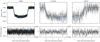 |
Fig. 1 Left: detrended and phase-folded TESS light curve of HD 2685 during the transit. The solid blue line corresponds to the transit fit from the joint analysis. Middle: LCOGT photometric data covering the ingress and middle part of one individual transit. Right: CHAT data covering the egress of the same transit event as observed by LCOGT. |
2 Observations and data analysis
2.1 TESS photometric data
HD 2685 (TIC 267263253, TOI 135) was observed in the high-cadence mode (two-minute exposures) in Sector 1 of the TESS space mission. These observations were collected by Camera 3 between July 25 and August 22, 2018. HD 2685 is not planned to be observed in other TESS sectors during the TESS primary mission. The light curve was processed by the Science Processing Operations Center (SPOC) pipeline (Jenkins et al. 2016), which is based on the Kepler Mission science pipeline (Jenkins 2017) and made available by the NASA Ames SPOC center and at the MAST archive2. This star was also listed by the TESS Alert system in Sector 1. The photometric dataset is comprised of a total of 18097 individual measurements, in which a total of 7 transit events were identified, with depths of ~ 10 000 ppm and duration of ~4.5 h. After masking out the transits, we detrended the light curve using a Gaussian process modeling, with the quasi-periodic kernel presented inForeman-Mackey et al. (2017). Figure 1 shows the detrended and phase-folded TESS light curve of HD 2685. The blue line corresponds to the best-fitting model described in Sect. 4.
2.2 CHAT photometry
In addition to the TESS photometric data, we also collected a total of 411 ground-based measurements using the Chilean-Hungarian Automated Telescope (CHAT; Jordán et al. 2019), installed at Las Campanas Observatory in Chile. Observations were acquired on September 22 UT of 2018 using the i’ sloan filter. The exposure time per image was 14 s, which translated into a cadence of ~ 25 s. A mild defocus was applied. The data were reduced through a dedicated automatic pipeline (Hartman et al. 2019; Jordán et al. 2019). The spatial resolution of CHAT (pixel scale of 0.6 arcsec) made these the first observations that helped us to confirm the source of the transit signal, discarding other potential sources in the TESS field of view. Figure 1 shows the CHAT photometry of HD 2685 during the transit. The residual scatter is 3105 and 1001 ppm when binned to five-minute bins. Even though the CHAT data only covered the second half of one transit event, the observed transit depth is consistent with the TESS data.
2.3 Las Cumbres Observatory photometry
We performed ground-based photometric follow-up using the Las Cumbres Observatory Global Telescope (LCOGT3) network (Brown et al. 2013). On 2018 September 22 UT, we observed an almost complete transit (missing the egress) in the I band using the LCOGT 0.4 m telescopes situated at South Africa Astronomical Observatory (SAAO) at Sutherland, South Africa. These observations were taken in the same night as the CHAT observations, meaning that we covered one full transit using two different instruments. The observations were made with the SBIG camera and consisted of 394 exposures with an exposure time of 30 s, taken while the telescope was defocused by 1.5 mm to spread the stellar point-spread function over more pixels, thereby reducing the effect of flat-fielding uncertainties. The data were reduced by the LCOGT pipeline, and photometry was carried out with AstroImageJ (Collins et al. 2017). The light curve is plotted in Fig. 1. The residual scatter is 2560 ppm per point and 786 ppm when binned to five-minute bins. These observations were made as part of an LCOGT Key Project to follow up TESS transiting planet candidates and characterize transiting planets using the LCOGT network4.
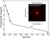 |
Fig. 2 Speckle autocorrelation function obtained in the I-band at the SOARtelescope. The black dots correspond to the 5σ contrast curve for HD 2685. The solid line corresponds to the linear fit of the data at separations smaller and larger than ~ 0.2′′. |
2.4 Speckle imaging
The relatively large 21′′ pixels of TESS can result in photometric contamination from nearby sources. These must be accounted for to rule out astrophysical false positives, such as background eclipsing binaries, and to correct the estimated planetary radius, initially derived from the diluted transit in a blended light curve. We searched for close companions to HD 2685 with I-band speckle imaging on the 4.1 m Southern Astrophysical Research (SOAR) telescope (Tokovinin 2018). The 5σ detection sensitivity and autocorrelation function of the observation are shown in Fig. 2. We detected no nearby stars down to a magnitude difference of ~4 mag at a separation of 0.2′′.
We additionally collected speckle imaging data using the Differential Speckle Survey Instrument (DSSI; Horch et al. 2009) at the 8 m Gemini South telescope. The target was simultaneously observed in the R and I filters. Figure 3 shows the reconstructed images and 5σ contrast curves in these two filters. No companion is detected to a magnitude contrast of ~4 mag at 0.2′′ of separation.
2.5 CHIRON radial velocities
As part of a two-week spectroscopic confirmation campaign of a handful of short-period transiting candidate planets detected by TESS, we obtained a total of 11 spectra of HD 2685 using CHIRON (Tokovinin et al. 2013), a fibre-fed high-resolution spectrograph mounted on the SMARTS 1.5 m telescope at the Cerro Tololo Inter-American Observatory in Chile. The spectra were taken using a 2.7′′ diameter fibre on sky, with the highly efficient image slicer mode. The exposure time was 1200 s, leading to a mean signal-to-noise-ratio (S/N) per pixel at 5500 Å of ~45. From the spectra, we computed relative RV measurements using the cross-correlation technique and corrected the night drift using Th-Ar spectra taken before and after each science exposure, as explained in Wang et al. (2019). This method was applied individually to a total of 41 orders covering the wavelength range between ~ 4500–7000 Å. The mean RV uncertainty per epoch is ~ 30 m s−1, explained mainly as due to the fast stellar rotation. The resulting RVs are plotted in Fig. 4 and are also listed in Table A.1. The resulting CHIRON RVs of HD 2685 revealed an amplitude of ≳ 100 m s−1, in phase with the orbital period detected in the TESS photometry. Additionally, from the cross-correlation-function (CCF), we computed the bisector velocity span (BVS), which is also listed in Table A.1. Figure 5 shows the BVS versus the RVs. While the BVS scatter is large, they do not show a correlation with the RVs. The Pearson correlation coefficient between the CHIRON BVS and RVs is − 0.14.
2.6 FEROS radial velocities
The CHIRON data were complemented with the Fiber-fed Extended Range Optical Spectrograph (FEROS; Kaufer et al. 1999) spectra using the simultaneous calibration technique (Baranne et al. 1996). In this mode, the 2.0′′ diameter science fibre is illuminated by the star, while the second fibre is illuminated by a Th-Ar reference lamp, which is used to correct for the RV drift. We obtained five spectra of HD 2685 with an exposure time of 300 s, leading to a mean S/N per resolution element of ≈100. The data reduction and RV calculation were performed with the CERES pipeline (Brahm et al. 2017a). The reduction process is relatively standard for echelle spectra and consists of a bias correction, flat-field order tracing, and optimal extraction. This method was applied to a total of 25 orders covering the wavelength region between ~ 3900–6800 Å. Finally, each order was wavelength calibrated. The wavelength solution is accurate at the ~ 2 m s−1 level and is obtained from a total ~1000 Th-Ar emission lines. The RVs were computed through a cross-correlation between each individual order with a binary numerical mask and were corrected for the night drift using the Th-Ar spectra. The resulting velocities are plotted in Fig. 4 and are listed in Table A.1. Similarly, we computed FEROS BVS values, which are also listed in Table A.1, and plot them in Fig. 5. There is no obvious correlation between these two quantities. The Pearson correlation coefficient between the FEROS BVS and the corresponding RVs is 0.24.
2.7 CORALIE radial velocities
Additional 14 spectra were obtained with the CORALIE high-resolution spectrograph on the Swiss 1.2 m Euler telescope at La Silla Observatory, Chile (Queloz et al. 2001), between 21 September and 28 October 2018. CORALIE is fed by a 2′′ science fibre and a secondary fibre with simultaneous Fabry–Perot for wavelength calibration. RVs were computed by cross-correlation with a binary G2 mask. Our exposures varied between 900 and 1800 s depending on the weather conditions. We obtained a final accuracy of 30–40 m s−1, which is limited by the stellar rotation due to broadening of the CCF. The resulting velocities are plotted in Fig. 4 and are listed in Table A.1. Additionally, we computed the BVS values at each observing epoch, which are also listed in Table A.1 and plotted in Fig. 4. The Pearson linear coefficient between the CORALIE RVs and BVS values is 0.01.
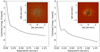 |
Fig. 3 Reconstructed DSSI images of HD 2685, obtained simultaneously in the R and I filters (left and right panel, respectively). The solid lines correspond to the 5σ contrast curves. |
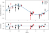 |
Fig. 4 Phase-folded RV curve of HD 2685. The black, red, and blue points correspond to CORALIE, CHIRON, and FEROS velocities, respectively. The best Keplerian fit from the joint analysis is overplotted. The post-fit residuals are shown in the lower panel. |
3 Host star properties
We first obtained the atmospheric parameters (Teff, log g, [Fe/H]) and the projected rotational velocity (v sin i) of HD 2685 from the coadded FEROS spectra using the ZASPE code (Brahm et al. 2017b). Briefly, ZASPE compares the stellar spectrum to the ATLAS9 grid of atmospheric models (Castelli & Kurucz 2004). This procedure is done in an iterative fashion, restricting the analysis to the spectral regions that are more sensitive to changes in the atmospheric parameters. Internal uncertainties and correlations between the parameters are obtained through Monte Carlo simulations that take into account systematic mismatches between the optimal model and the observed spectrum.
In the second step, we computed the stellar radius (R⋆) and the visual extinction coefficient (AV), following the method described in Brahm et al. (2018). For this, we used the BT-Settl-CIFIST models (Baraffe et al. 2015) to generate a spectral energy distribution (SED) whose parameters are equal to those derived in the spectroscopic analysis. Using the SED and the stellar distance from the Gaia parallax, we computed synthetic apparent magnitudes, which were compared to the observed ones (listed in Table 1) to derive R⋆ and AV 5. The parameter space was explored with the EMCEE package (Foreman-Mackey et al. 2013).
Finally, to obtain the mass, age, and luminosity of the star, we compared its derived effective temperature and radius to that predicted bythe Yonsei–Yale isochrones (Yi et al. 2001) for different masses and evolutionary stages by fixing the metallicity of the isochrones to the value obtained in the spectroscopic analysis. Again, the parameter space was explored using the emcee package. Through estimating the stellar mass and radius, this procedure allows us to estimate a more precise value of log g than can beobtained with the spectroscopic analysis. Therefore, we performed a new ZASPE run fixing log g to the value obtained from R⋆ and M⋆, and then we also repeated thedetermination of these physical parameters. Using this method, we obtained the following atmospheric parameters for HD 2685: Teff = 6801 ± 76, log g = 4.21 ± 0.03 cm s−2, [Fe/H] = +0.02 ± 0.06 dex, and v sin i = 15.4 ± 0.2 km s−1. We note that to account for systematics, we added in quadrature to the internal uncertainties 50 K, 0.03 and 0.05 dex in Teff, log g, and [Fe/H], respectively. We also found a value of AV 0.09 ± 0.05 mag. Similarly, we obtained the following physical parameters for HD 2685 : M⋆ = 1.43  M⊙, R⋆ = 1.56 ± 0.05 R⊙, L⋆ = 4.66
  L⊙, and age = 1.31
  Gyr. The atmospheric and physical parameters are listed in Table 1 and are adopted for the rest of the paper.
For comparison, we also derived the stellar atmospheric parameters following the method presented in Jones et al. (2011) and Wang et al. (2019). Briefly, we used ARES v2 (Sousa et al. 2015) to measure the equivalent width (EW) of ~ 150 Fe I and Fe II absorption lines from the coadded CHIRON template. These resulting EWs were then compared to the synthetic EWs generated by the MOOG code (Sneden 1973), which solves the radiative transfer equations under the assumptions of local thermodynamic equilibrium, using the Kurucz (1993) stellar atmosphere models. From this analysis, we obtained the following atmospheric parameters for HD 2685: Teff = 6800 ± 70 K, log g = 4.15 ± 0.15, and [Fe/H] = –0.08 ± 0.10, which are in good agreement with those derived by ZASPE.
Finally, we also performed an analysis of the broadband SED of HD 2685 together with the Gaia DR2 parallax in order to determine an empirical measurement of the stellar radius, following Stassun et al. (2018). For this, we used the BT VT magnitudes from Tycho-2, the Strömgren ubvy magnitudes from Paunzen (2015), the BV gri magnitudes from APASS, the JHKS magnitudes from 2MASS, the W1–W4 magnitudes from WISE, and the G magnitude from Gaia. We performed a fit using Kurucz stellar atmosphere models, for which the free parameters were the effective temperature, the surface gravity, the metallicity, and the extinction, which we restricted to the maximum line-of-sight value from the dust maps of Schlegel et al. (1998). The best-fit parameters are Teff = 6800 ± 100 K, log g = 4.0 ± 0.25, [Fe/H] = 0.00 ± 0.25, and AV = 0.09 ± 0.02. These values are consistent with those determined from the spectroscopic analysis. Finally, taking the stellar bolometric flux computed from the unreddened model SED, and Teff together with the Gaia DR2 parallax yields a stellar radius of R = 1.57 ± 0.03 R⊙, which agrees excellently with that determined from the ZASPE code.
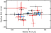 |
Fig. 5 Bisector velocity span as functions of the CORALIE (black dots), CHIRON (red dots), and FEROS (blue dots) radial velocities. An arbitrary offset is applied to the BVS values. |
Stellar parameters.
4 Global analysis
We performed a global analysis using both the photometric and spectroscopic data. To do this, we used the EXOplanet traNsits and rAdiAl veLocity fittER (EXONAILER), which is described in detail in Espinoza et al. (2016) and is available at GitHub6. Briefly, we modeled the detrended light curve using the BATMAN code (Kreidberg 2015) by simultaneously fitting the limb-darkening coefficients with the rest of the transit parameters, following the quadratic limb-darkening law presented in Espinoza & Jordán (2016) and using the sampling scheme from Kipping (2013). Similarly, the RV measurements were modeled using the RAD-VEL package (Fulton et al. 2018). For the RVs, we included a jitter and RV offset as a free parameter for each RV dataset. Table 2 lists the resulting transit values and the derived planetary parameters. Finally, from the derived stellar and planetary parameters, we computed the equilibrium temperature (Teq) for HD 2685 b. By adopting a zero albedo and assuming a tidally locked planet with no heat distribution (β = 0.5; Kaltenegger & Sasselov 2011), we obtained Teq = 2061 ± 28 K for HD 2685 b.
In addition, we have examined the phase-folded light curve for any variability outside of the transit, including orbital phase curves (Shporer 2017) and secondary eclipse. We did not detect any sinusoidal variation along the orbital phase, which is expected given the system parameters and the sensitivity of the data. We attempted to measure the secondary eclipse, assuming that its duration is identical to that of the transit and that it takes place exactly half an orbital period away from it. We measured a depth of 17 ± 23 ppm, meaning that we did not detect the secondary eclipse and are able to place a 3σ upper limit of 69 ppm on its depth (or a 2σ upper limit of 46 ppm). This translates into a 3σ upper limit on the geometric albedo in the TESS band of Ag < 0.47 (or a 2σ upper limit of 0.31). This upper limit is consistent with the low geometric albedos found for hot-Jupiter exoplanets in visible light (e.g. Heng & Demory 2013; Shporer et al. 2014; Esteves et al. 2015; Angerhausen et al. 2015). In the above we have assumed that the thermal emission contributes little or negligibly to the secondary eclipse, which in this system reaches only 12 ppm in the extreme case of no heat circulation between the day to night planet hemispheres.
5 Discussion
We have presented the radial velocity confirmation of HD 2685 b, a transiting hot Jupiter observed in Sector 1 of the TESS mission. We obtained CHIRON, CORALIE, and FEROS spectroscopic data, from which we confirmed the planetary nature of the transit signal detected by TESS. In addition, we obtained CHAT and LCOGT photometric data during one transit event. From the joint analysis we derived the following parameters for HD 2685 b: P = 4.12688 days, Mp = 1.17 ± 0.12 MJ, and Rp = 1.44 ± 0.05 RJ. We also measured a low eccentricity (e = 0.091
 ), which is consistent with a circular orbit at the 2σ level.
Figure 6 shows the planetary radius versus mass for known transiting gas giants. The red dot corresponds to HD 2685 b. Different isodensity contours are overplotted (dashed gray lines). Also for comparison, the solid lines mark theoretical models from Baraffe et al. (2014) for no solid coreand 100 M⊕ core planets. Similarly, Fig. 7 shows the planetary radius versus the planet’s equilibrium temperature. These two plots clearly show that HD 2685 b is an inflated hot Jupiter, whose large radius cannot be explained by current theoretical models of planetary internal structure (e.g. Baraffe et al. 2014), but may probably be explained by the high irradiation received by the parent star (e.g. Hartman et al. 2011; Weiss et al. 2013).
Figure 8 shows the position of HD 2685 in the stellar log (g) versus Teff parameter space for transiting planets host stars. HD 2685 is one of the hottest stars with a known transiting gas giant planet, with only about a dozen host stars at a similar temperature or hotter.
Finally, HD 2685 has a visual magnitude of V = 9.6 mag, meaning that it is one of the brightest stars with a transiting giant planet. This makes it a valuable target for detailed follow-up characterization.
In addition to its high apparent brightness (V = 9.6 mag), HD 2685 is a relatively hot (Teff = 6801 ± 76 K) and fast-rotating star (v sin i = 15.4 ± 0.2 km s−1), making this object an excellent target for studying the projected spin-orbit angle through the Rossiter–McLaughlin effect. Knowing the stellar obliquity in transiting giant planets can give us important information about different planetary migration processes. While some of these mechanisms predict a damping in the spin-orbit primordial misalignment, if any (Cresswell et al. 2007), some others are expected to alter the mutual inclination angle (e.g. Fabrycky &Tremaine 2007). For this reason, knowing the obliquity angle can help us to distinguish between different migrations scenarios (Wang et al. 2018). Moreover, Winn et al. (2010) showed that hotter stars (Teff ≳ 6250 K) hosting hot Jupiters have a higher obliquity than cooler stars. Based on this result, HD 2685 b might be expected to be in a high-obliquity orbit. Based on the derived stellar and planet parameters, we predict an RV semi-amplitude during the transit of ≈92 m s−1 (assuming an aligned orbit), which can be easily detected given the RV precision attained for this object. Thus this target provides us with an excellent opportunity to further study this observational trend in the high Teff regime (see Addison et al. 2018 for an updated version of this correlation).
On the other hand, transiting exoplanets around bright stars provide a great laboratory for probing physical properties of these alien worlds. Arguably, the most intriguing and accessible of these characteristics is their atmospheric makeup. Studying exoplanetary atmospheres gives us clues about the formation and evolution history of the planetary system, the composition of the initial protoplanetary disk in which the planet was formed, the location of that formation (Madhusudhan et al. 2014; Mordasini et al. 2016), and the internal structure of the planet (Dorn et al. 2015). There are a variety of techniques through which minute signatures of exoplanetary atmospheres are detected. The most effective of these has been transmission spectroscopy, which searches for atmospheric imprints on the traversing stellar light (Seager & Sessalov 2000). This is mainly donethrough either performing mid-to-low resolution highly time-resolved spectroscopy using multi-object spectrographs from the ground (e.g. FORS2; Bean et al. 2011, Sedaghati et al. 2017, IMACS; Jordán et al. 2013, Espinoza et al. 2019), space (e.g. HST and Spitzer; Sing et al. 2016), or high-resolution stable spectroscopy (e.g. HARPS; Allart et al. 2017). The significance of the detection of various atomic and/or molecular species heavily relies on thebrightness of the host star and on the scale height of the exoatmosphere being probed. Consequently, HD 2685 b is an ideal candidate for atmospheric follow-up studies on both accounts. The 9.6 visual magnitude of the host star allows for obtaining high S/N spectra with relatively short exposure times, which are essential for performing transmission spectroscopy. Additionally, assuming a H/He-dominated atmosphere, the extended scale height of the atmosphere ( km) due to the high equilibrium temperature expected, leads to significant atmospheric signals that are well within the reach of current and future instrumentation (e.g. ESPRESSO and the JWST).
Parameters obtained from the global modeling.
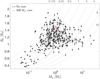 |
Fig. 6 Planet radius-mass diagram for transiting gas giant planets. The mass axis is plotted in logarithmic scale. The solid lines mark theoretical models taken from Baraffe et al. (2014) for no solid core (black) and a massive core of 100 MEarth (gray). The dashed lines mark isodensity contours, with the density values labeled at the top right corner in g cm−3. The positionof HD 2685 b shows that it is an inflated gas giant planet, like other planets of similar mass. The plot includes planets whose radius uncertainty is smaller than 0.15 RJ and whose mass uncertainty is smaller than a quarter of the measured mass. Data presented in this plot were obtained from the NASA Exoplanet Archive (Akeson et al. 2013) on January 24, 2019. |
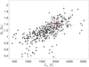 |
Fig. 7 Planet radius vs. equilibrium temperature, showing the well-known correlation between the two parameters. The position of HD 2685 b, marked in red, is in good agreement with this correlation. The plot includes planets whose radius uncertainty is smaller than 0.15 RJ and whose mass uncertainty is smaller than a quarter of the measured mass. Data presented in this plot were obtained from the NASA Exoplanet Archive (Akeson et al. 2013) on January 24, 2019. |
 |
Fig. 8 Stellar surface gravity (in cgs units) vs. effective temperature of all known transiting planet host stars where the planetary mass and radius are both measured. The red dot shows the position of HD 2685. Data presented in this plot were obtained from the NASA Exoplanet Archive (Akeson et al. 2013) on January 24, 2019. |
Acknowledgements
S.W. and J.N.W. thank the Heising-Simons Foundation for their generous support. C.Z. is supported by a Dunlap Fellowship at the Dunlap Institute for Astronomy & Astrophysics, funded through an endowment established by the Dunlap family and the University of Toronto. A.V.’s work was performed under contract with the California Institute of Technology (Caltech)/Jet Propulsion Laboratory (JPL) funded by NASA through the Sagan Fellowship Program executed by the NASA Exoplanet Science Institute. A.J. acknowledges support from FONDECYT project 1171208, CONICYT project Basal AFB-170002, and by the Ministry for the Economy, Development, and Tourism’s Programa Iniciativa Científica Milenio through grant IC 120009, awarded to the Millennium Institute of Astrophysics (MAS). We acknowledge the use of TESS Alert data, which is currently in a beta test phase, from pipelines at the TESS Science Office and at the TESS Science Processing Operations Center. This research has made use of the Exoplanet Follow-up Observation Program website, which is operated by the California Institute of Technology, under contract with the National Aeronautics and Space Administration under the Exoplanet Exploration Program. This paper includes data collected by the TESS mission, which are publicly available from the Mikulski Archive for Space Telescopes (MAST). This work makes use of observations from the LCOGT network.
Appendix A Radial velocities
Relative radial velocities of HD 2685.
References
- Addison, B. C., Wang, S., Johnson, M. C., et al. 2018, AJ, 156, 197 [NASA ADS] [CrossRef] [Google Scholar]
- Akeson, R. L., Chen, X., Ciardi, D., et al. 2013, PASP, 125, 989 [NASA ADS] [CrossRef] [Google Scholar]
- Allart, R., Lovis, C., Pino, L., et al. 2017, A&A, 606, 144 [Google Scholar]
- Angerhausen, D., DeLarme, E., & Morse, J. A. 2015, PASP, 127, 1113 [NASA ADS] [CrossRef] [Google Scholar]
- Baraffe, I., Chabrier, G., Fortney, J., & Sotin, C. 2014, Protostars and Planets VI (Tucson: University of Arizona Press), 763 [Google Scholar]
- Baraffe, I., Homeier, D., Allard, F., & Chabrier, G. 2015, A&A, 577, A42 [NASA ADS] [CrossRef] [EDP Sciences] [Google Scholar]
- Baranne, A., Queloz, D., Mayor, M., et al. 1996, A&A, 119, 373 [Google Scholar]
- Barclay, T., Pepper, J., & Quintana, E. 2018, ApJS, 239, 2 [NASA ADS] [CrossRef] [Google Scholar]
- Bean, J. L., Désert, J.-M., Kabath, P., et al. 2011, ApJ, 732, 92 [NASA ADS] [CrossRef] [Google Scholar]
- Benneke, B., & Seager, S. 2012, ApJ, 753, 100 [NASA ADS] [CrossRef] [Google Scholar]
- Borucki, W. J., Koch, D., Basri, G., et al. 2010, Science, 327, 977 [NASA ADS] [CrossRef] [PubMed] [Google Scholar]
- Brahm, R., Jordán, A., & Espinoza, N. 2017a, PASP, 129, 34002 [Google Scholar]
- Brahm, R., Jordán, A., Hartman, J., & Bakos, G. 2017b, MNRAS, 467, 971 [NASA ADS] [Google Scholar]
- Brahm, R., Espinoza, N., Jordán, A., et al. 2018, MNRAS, 477, 2572 [NASA ADS] [CrossRef] [Google Scholar]
- Broeg, C., Fortier, A., Ehrenreich, D., et al. 2013, Eur. Phys. J. Web Conf. 47, 03005 [CrossRef] [EDP Sciences] [Google Scholar]
- Brown, T. M., Baliber, N., Bianco, F. B., et al. 2013, PASP, 125, 1031 [NASA ADS] [CrossRef] [Google Scholar]
- Cardelli, J. A., Clayton, G. C., & Mathis, J. S. 1989, ApJ, 345, 245 [NASA ADS] [CrossRef] [Google Scholar]
- Castelli, F., & Kurucz, R. L. 2004, ArXiv e-prints [arXiv:astro-ph/0405087] [Google Scholar]
- Collins, K. A., Kielkopf, J. F., Stassun, K. G., & Hessman, F. V. 2017, AJ, 153, 77 [NASA ADS] [CrossRef] [Google Scholar]
- Cresswell, P., Dirksen, G., Kley, W., & Nelson, R. P. 2007, A&A, 473, 329 [NASA ADS] [CrossRef] [EDP Sciences] [Google Scholar]
- Dorn, C., Khan, A., Heng, K., et al. 2015, A&A, 577, 83 [Google Scholar]
- Dressing, C. D., & Charbonneau, D. 2013, ApJ, 767, 95 [NASA ADS] [CrossRef] [Google Scholar]
- Espinoza, N., & Jordán, A. 2016, MNRAS, 457, 3573 [NASA ADS] [CrossRef] [Google Scholar]
- Espinoza, N., Brahm, R., Jordán, A., et al. 2016, ApJ, 830, 43 [NASA ADS] [CrossRef] [Google Scholar]
- Espinoza, N., Rackham, B. V., Jordán, A., et al. 2019, MNRAS, 482, 2065 [Google Scholar]
- Esteves, L. J., De Mooij, E. J. W., & Jayawardhana, R. 2015, ApJ, 804, 150 [NASA ADS] [CrossRef] [Google Scholar]
- Fabrycky, D., & Tremaine, S. 2007, ApJ, 669, 1298 [NASA ADS] [CrossRef] [Google Scholar]
- Foreman-Mackey, D., Hogg, D. W., Lang, D., & Goodman, J. 2013, PASP, 125, 306 [CrossRef] [Google Scholar]
- Foreman-Mackey, D., Agol, E., Ambikasaran, S., & Angus, R. 2017, AJ, 154, 220 [NASA ADS] [CrossRef] [Google Scholar]
- Fulton, B. J., Petigura, E. A., & Blunt, S., Sinukoff, E. 2018, PASP, 130, 986 [Google Scholar]
- Gaia Collaboration (Brown, A. G. A., et al.) 2018, A&A, 616, A1 [NASA ADS] [CrossRef] [EDP Sciences] [Google Scholar]
- Gandolfi, D., Barragán, O., Livingston, J. H., et al. 2018, A&A, 619, L10 [NASA ADS] [CrossRef] [EDP Sciences] [Google Scholar]
- Gardner, J. P., Mather, J. C., Clampin, M., et al. 2006, Space Sci. Rev. 123, 485 [NASA ADS] [CrossRef] [Google Scholar]
- Guillot, T., & Showman, A. P. 2002, A&A, 385, 156 [NASA ADS] [CrossRef] [EDP Sciences] [Google Scholar]
- Hartman, J. D., Bakos, G. Á., Torres, G., et al. 2011, ApJ, 742, 59 [NASA ADS] [CrossRef] [Google Scholar]
- Hartman, J. D., Bakos, G. Á., Bayliss, D., et al. 2019, AJ, 157, 55 [NASA ADS] [CrossRef] [Google Scholar]
- Heng, K., & Demory, B.-O. 2013, ApJ, 777, 100 [NASA ADS] [CrossRef] [Google Scholar]
- Horch, E. P., Veillette, D. R., Baena, G., et al. 2009, AJ, 137, 5057 [NASA ADS] [CrossRef] [Google Scholar]
- Huang, C. X., Burt, J., Vanderburg, A., et al. 2018, ApJ, 868, L39 [NASA ADS] [CrossRef] [Google Scholar]
- Jenkins, J. M. 2017, Kepler Data Processing Handbook, KSCI-19081-002 [Google Scholar]
- Jenkins, J. M., Twicken, J. D., McCauliff, S., et al. 2016, in Software and Cyberinfrastructure for Astronomy IV, Proc. SPIE, 9913, 99133E [Google Scholar]
- Jones, M. I., Jenkins, J. S., Rojo, P., & Melo, C. H. F. 2011, A&A, 536, A71 [NASA ADS] [CrossRef] [EDP Sciences] [Google Scholar]
- Jones, M. I., Brahm, R., Wittenmyer, R. A., et al. 2017, A&A, 602, 58 [Google Scholar]
- Jordán, A., Espinoza, N., Rabus, M., et al. 2013, ApJ, 778, 184 [NASA ADS] [CrossRef] [Google Scholar]
- Jordán, A., Brahm, R., Espinoza, N., et al. 2019, AJ, 157, 100 [NASA ADS] [CrossRef] [Google Scholar]
- Kaltenegger, L., & Sasselov, D. 2011, ApJ, 736, L25 [NASA ADS] [CrossRef] [Google Scholar]
- Kaufer, A., Stahl, O., Tubbesing, S. et al. 1999, The Messenger, 95, 8 [Google Scholar]
- Kipping, D. M. 2013, MNRAS, 435, 2152 [Google Scholar]
- Kreidberg, L. 2015, PASP, 127, 1161 [NASA ADS] [CrossRef] [Google Scholar]
- Kurucz, R. 1993, ATLAS9 Stellar Atmosphere Programs and 2 km/s grid. Kurucz CD-ROM No. 13. (Cambridge, MA: Smithsonian Astrophysical Observatory), 1993 [Google Scholar]
- Madhusudhan, N., Amin, M. A., & Kennedy, G. M. 2014, ApJ, 794, L12 [Google Scholar]
- Matsumura, S., Peale, S. J., & Rasio, F. A. 2010, ApJ, 725, 1995 [NASA ADS] [CrossRef] [Google Scholar]
- Mordasini, C., van Boekel, R., Molliere, P., et al. 2016, ApJ, 832, 41 [NASA ADS] [CrossRef] [Google Scholar]
- Mulders, G. D., Pascucci, I., & Apai, D. 2015, ApJ, 814, 130 [NASA ADS] [CrossRef] [Google Scholar]
- Paunzen, E. 2015, A&A, 580, A23 [NASA ADS] [CrossRef] [EDP Sciences] [Google Scholar]
- Queloz, D., Eggenberger, A., Mayor, M., et al. 2000, A&A, 359, L13 [NASA ADS] [Google Scholar]
- Queloz, D., Mayor, M., Udry, S., et al. 2001, The Messenger, 105, 1 [NASA ADS] [Google Scholar]
- Rasio, F. A., Tout, C. A., Lubow, S. H., & Livio, M. 1996, ApJ, 470, 1187 [NASA ADS] [CrossRef] [Google Scholar]
- Ricker, G. R., Winn, J. N., Vanderspek, R., et al. 2015, J. Astron. Telesc. Instrum. Syst., 1, 014003 [NASA ADS] [CrossRef] [Google Scholar]
- Schlegel, D. J., Finkbeiner, D. P., & Davis, M. 1998, ApJ, 500, 525 [NASA ADS] [CrossRef] [Google Scholar]
- Seager, S., & Sessalov, D. D. 2000, ApJ, 537, 916 [NASA ADS] [CrossRef] [Google Scholar]
- Sedaghati, E., Boffin, H. M. J., MacDonald, R. J., et al. 2017, Nature, 549, 238 [NASA ADS] [CrossRef] [Google Scholar]
- Shporer, A. 2017, PASP, 129, 072001 [NASA ADS] [CrossRef] [Google Scholar]
- Shporer, A., O’Rourke, J. G., Knutson, H. A., et al. 2014, ApJ, 788, 92 [NASA ADS] [CrossRef] [Google Scholar]
- Sing, D. K., Fortney, J. J., Nikolov, N., et al. 2016, Nature, 529, 59 [NASA ADS] [CrossRef] [Google Scholar]
- Sneden, C. 1973, ApJ, 184, 839 [NASA ADS] [CrossRef] [Google Scholar]
- Snellen, I. A. G., de Kok, R. J., le Poole, R., Brogi, M., & Birkby, J. 2013, ApJ, 764, 182 [NASA ADS] [CrossRef] [Google Scholar]
- Sousa, S. G., Santos, N. C., Adibekyan, V., Delgado-Mena, E., & Israelian, G. 2015, A&A, 577, A67 [NASA ADS] [CrossRef] [EDP Sciences] [Google Scholar]
- Stassun, K. G., Corsaro, E., Pepper, J. A., & Gaudi, B. S. 2018, AJ, 155, 22 [NASA ADS] [CrossRef] [Google Scholar]
- Thorngren, D. P., Fortney, J. J., Murray-Clay, R. A., & Lopez, E. D. 2016, ApJ, 831, 64 [NASA ADS] [CrossRef] [Google Scholar]
- Tokovinin, A. 2018, PASP, 130, 35002 [Google Scholar]
- Tokovinin, A., Fischer, D. A., Bonati, M., et al. 2013, PASP, 125, 1336 [NASA ADS] [CrossRef] [Google Scholar]
- Wang, S., Addison, B., Fischer, D. A., et al. 2018, AJ, 155, 70 [NASA ADS] [CrossRef] [Google Scholar]
- Wang, S., Jones, M., Shporer, A., et al. 2019, AJ, 157, 51 [NASA ADS] [CrossRef] [Google Scholar]
- Weiss, L. M., Marcy, G. W., Rowe, J. F., et al. 2013, ApJ, 768, 14 [NASA ADS] [CrossRef] [Google Scholar]
- Winn, J. N., & Fabrycky, D. C. 2015, ARA&A, 53, 409 [NASA ADS] [CrossRef] [Google Scholar]
- Winn, J. N., Fabrycky, D., Albrecht, S., & Johnson, J. A. 2010, ApJ, 718, L145 [NASA ADS] [CrossRef] [Google Scholar]
- Yi, S., Demarque, P., Kim, Y.-C., et al. 2001, ApJS, 136, 417 [NASA ADS] [CrossRef] [Google Scholar]
For different filters we obtain Aλ from AV, adopting the Cardelli et al. (1989) extinction law.
All Tables
All Figures
|
Fig. 1 Left: detrended and phase-folded TESS light curve of HD 2685 during the transit. The solid blue line corresponds to the transit fit from the joint analysis. Middle: LCOGT photometric data covering the ingress and middle part of one individual transit. Right: CHAT data covering the egress of the same transit event as observed by LCOGT. |
| In the text | |
|
Fig. 2 Speckle autocorrelation function obtained in the I-band at the SOARtelescope. The black dots correspond to the 5σ contrast curve for HD 2685. The solid line corresponds to the linear fit of the data at separations smaller and larger than ~ 0.2′′. |
| In the text | |
|
Fig. 3 Reconstructed DSSI images of HD 2685, obtained simultaneously in the R and I filters (left and right panel, respectively). The solid lines correspond to the 5σ contrast curves. |
| In the text | |
|
Fig. 4 Phase-folded RV curve of HD 2685. The black, red, and blue points correspond to CORALIE, CHIRON, and FEROS velocities, respectively. The best Keplerian fit from the joint analysis is overplotted. The post-fit residuals are shown in the lower panel. |
| In the text | |
|
Fig. 5 Bisector velocity span as functions of the CORALIE (black dots), CHIRON (red dots), and FEROS (blue dots) radial velocities. An arbitrary offset is applied to the BVS values. |
| In the text | |
|
Fig. 6 Planet radius-mass diagram for transiting gas giant planets. The mass axis is plotted in logarithmic scale. The solid lines mark theoretical models taken from Baraffe et al. (2014) for no solid core (black) and a massive core of 100 MEarth (gray). The dashed lines mark isodensity contours, with the density values labeled at the top right corner in g cm−3. The positionof HD 2685 b shows that it is an inflated gas giant planet, like other planets of similar mass. The plot includes planets whose radius uncertainty is smaller than 0.15 RJ and whose mass uncertainty is smaller than a quarter of the measured mass. Data presented in this plot were obtained from the NASA Exoplanet Archive (Akeson et al. 2013) on January 24, 2019. |
| In the text | |
|
Fig. 7 Planet radius vs. equilibrium temperature, showing the well-known correlation between the two parameters. The position of HD 2685 b, marked in red, is in good agreement with this correlation. The plot includes planets whose radius uncertainty is smaller than 0.15 RJ and whose mass uncertainty is smaller than a quarter of the measured mass. Data presented in this plot were obtained from the NASA Exoplanet Archive (Akeson et al. 2013) on January 24, 2019. |
| In the text | |
|
Fig. 8 Stellar surface gravity (in cgs units) vs. effective temperature of all known transiting planet host stars where the planetary mass and radius are both measured. The red dot shows the position of HD 2685. Data presented in this plot were obtained from the NASA Exoplanet Archive (Akeson et al. 2013) on January 24, 2019. |
| In the text | |
Current usage metrics show cumulative count of Article Views (full-text article views including HTML views, PDF and ePub downloads, according to the available data) and Abstracts Views on Vision4Press platform.
Data correspond to usage on the plateform after 2015. The current usage metrics is available 48-96 hours after online publication and is updated daily on week days.
Initial download of the metrics may take a while.