| Issue |
A&A
Volume 624, April 2019
|
|
|---|---|---|
| Article Number | A125 | |
| Number of page(s) | 14 | |
| Section | Extragalactic astronomy | |
| DOI | https://doi.org/10.1051/0004-6361/201935106 | |
| Published online | 24 April 2019 | |
Spatially resolved carbon and oxygen isotopic ratios in NGC 253 using optically thin tracers
1
European Southern Observatory, Alonso de Córdova, 3107, Vitacura, Santiago 763-0355, Chile
e-mail: This email address is being protected from spambots. You need JavaScript enabled to view it.
2
Joint ALMA Observatory, Alonso de Córdova, 3107, Vitacura, Santiago 763-0355, Chile
3
Department of Space, Earth and Environment, Chalmers University of Technology, Onsala Space Observatory, 43992 Onsala, Sweden
4
Max-Planck-Institut für Radioastronomie, Auf dem Hugel 69, 53121 Bonn, Germany
5
Astron. Dept., King Abdulaziz University, PO Box 80203 Jeddah 21589, Saudi Arabia
6
New Mexico Institute of Mining and Technology, 801 Leroy Place, Socorro, NM 87801, USA
7
National Radio Astronomy Observatory, PO Box O, 1003 Lopezville Road, Socorro, NM 87801, USA
8
Institute of Astronomy and Astrophysics, Academia Sinica, PO Box 23-141, 10617 Taipei, Taiwan
9
Leiden Observatory, Leiden University, PO Box 9513, 2300 RA Leiden, The Netherlands
Received:
22
January
2019
Accepted:
6
March
2019
Abstract
Context. One of the most important aspects of modern astrophysics is related to our understanding of the origin of elements and chemical evolution in the large variety of astronomical sources. Nuclear regions of galaxies undergo heavy processing of matter, and are therefore ideal targets to investigate matter cycles via determination of elemental and isotopic abundances.
Aims. To trace chemical evolution in a prototypical starburst environment, we spatially resolve carbon and oxygen isotope ratios across the central molecular zone (CMZ; full size ∼600 pc) in the nearby starburst galaxy NGC 253.
Methods. We imaged the emission of the optically thin isotopologues 13CO, C18O, C17O, 13C18O at a spatial resolution ∼50 pc, comparable to the typical size of giant molecular associations. Optical depth effects and contamination of 13C18O by C4H are discussed and accounted for to derive column densities.
Results. This is the first extragalactic detection of the double isotopologue 13C18O. Derived isotopic ratios 12C/13C ∼ 21 ± 6, 16O/18O ∼ 130 ± 40, and 18O/17O ∼ 4.5 ± 0.8 differ from the generally adopted values in the nuclei of galaxies.
Conclusions. The molecular clouds in the central region of NGC 253 show similar rare isotope enrichment to those within the CMZ of the Milky way. This enrichment is attributed to stellar nucleosynthesis. Measured isotopic ratios suggest an enhancement of 18O as compared to our Galactic centre, which we attribute to an extra 18O injection from massive stars. Our observations show evidence for mixing of distinct gas components with different degrees of processing. We observe an extra molecular component of highly processed gas on top of the already proposed less processed gas being transported to the central region of NGC 253. Such a multicomponent nature and optical depth effects may hinder the use of isotopic ratios based on a spatially unresolved line to infer the star formation history and/or initial stellar mass function properties galaxy nuclei.
Key words: line: identification / ISM: molecules / ISM: abundances / Galaxy: abundances / galaxies: individual: NGC 253 / galaxies: starburst
© ESO 2019
1. Introduction
Interstellar isotope ratios carry essential information on the processes of nucleosynthesis in the hot and dense interior of stars. Measuring isotopic abundances such as 12C/13C and 18O/17O in the nuclear regions of starburst galaxies can therefore reveal the fingerprint of their star formation history. Isotopic ratios can be also be related to the relative contribution of high-mass to intermediate-mass stellar processing (Zhang et al. 2015). Thus these ratios can serve as tracers of the chemical evolution of the interstellar medium (ISM) due to stellar processing. The recent work by Romano et al. (2017) has attempted to model the available isotopic ratios observed in galaxies as a function of the star forming history and the stellar initial mass function (IMF). Based on their comparison of observations and model results they find evidence of a top-heavy IMF responsible for the observed ratios in starburst galaxies.
However, measuring isotopic ratios in astronomical sources is not always straightforward. At optical wavelengths, such measurements are difficult or impossible owing to the blending of atomic isotope lines and isotope specific obscuration from dust grains. Isotopic measurements of atomic carbon in the far-infrared and carbon monoxide in the near-infrared have been obtained (i.e. Goto et al. 2003, and references therein). On the other hand, observations of molecular isotopologues at radio to submillimeter wavelengths have been proven most successful within the Galaxy, towards the local extragalactic ISM (see Martín et al. 2010; Henkel et al. 2014; Romano et al. 2017, and references therein), and all the way to high redshift molecular absorbers (i.e., Muller et al. 2011; Wallström et al. 2016).
In this paper we focus on the isotopic ratio of 12C to 16O, as primary products of stellar nucleosynthesis, and the rarer 13C, 18O, and 17O, as secondary nuclear products from primary seeds (Meyer 1994; Wilson & Matteucci 1992; Wilson & Rood 1994). We note that, primary production of 13C and 18O is predicted for fast-rotating low metallicity massive stars and intermediate-mass stars climbing the asymptotic giant branch (Chiappini et al. 2008; Karakas & Lattanzio 2014; Limongi & Chieffi 2018), but the former results in a relatively small enrichment while the latter will not be relevant for the overall galactic scales involved in this work. In this context, when referring to enrichment we mean rare isotopologues enrichment, and therefore lower 12C/13C, 16O/18O, and 18O/17O isotopic ratios. As compiled in Wilson & Rood (1994) and Henkel et al. (1994), the generally adopted values in the nuclei of low luminosity local starbursts are 12C/13C ∼ 40, 16O/18O ∼ 200, and 18O/17O ∼ 8 (Sage et al. 1991; Henkel et al. 1993; Henkel & Mauersberger 1993). These ratios are derived from C- and O-bearing molecular species commonly observed in the ISM, such as CO, CN, CS, HCN, HNC, and HCO+, which, despite not suffering from line blending between the main and rare isotopologues, may actually be biased by optical depth effects. These limitations result in most of the cited ratios to be lower limits. To circumvent this problem, it is sometimes possible to turn to rare isotopologues involving another element, for example studying the double ratio 12C34S/13C32S, but this adds potential problems due to poor understanding of the extra isotopic ratio (in this example, 32S/34S, Henkel et al. 2014; Meier et al. 2015).
Recently, Henkel et al. (2014) used high quality spectra of CN towards the starburst galaxy NGC 253 to revisit its 12C/13C ratio. Thanks to the hyperfine splitting of CN, it is possible to estimate the optical depth of the main isotopologue. The resulting 12C/13C ∼ 40 ± 10 confirmed some of the previous estimates. An accurate measurement of the 12C/13C ratio also becomes important because this ratio is often used to derive other atomic isotopic ratios based on observations of the optically thinner 13C bearing isotopologues (i.e., Martín et al. 2005).
However, there are several non-local thermodynamic equilibrium (non-LTE) effects that can affect the observed molecular line ratios based on optically thick species (Meier & Turner 2001; Meier et al. 2015). As pointed out by Wilson & Rood (1994), in order to minimize effects such as optical thickness of the emission, excitation differences due to resonant photon trapping and/or selective photodissociation, we would rather choose the observation of optically thin isotopologues such as C18O and 13C18O. Despite the weakness of the emission of these isotopologues, observations have been successfully performed across the Galaxy (Langer & Penzias 1990; Ikeda et al. 2002), but are very challenging in extragalactic sources. High sensitivity observations with the IRAM 30 m telescope were carried out by Martín et al. (2010) in an attempt to detect 13C18O towards the nearby starburst galaxies NGC 253 and M 82. The resulting tentative detection towards NGC 253 yielded a lower limit of 12C/13C ≳ 60, which is comparatively higher than previous estimates.
Another important effect to take into account is that of isotopic fractionation (Watson 1977; Langer et al. 1984; Wilson & Rood 1994; Röllig & Ossenkopf 2013; Szűcs et al. 2014; Roueff et al. 2015), in which the unbalance of exothermic isotope exchange chemical reactions may favour the enhancement of the rarer isotopologues. The most relevant isotope barrierless fractionation reactions for the carbon monoxide species studied in this paper are written as
 (1)
(1)
where the heats of the reaction are ΔE1 = 35 K, ΔE2 = 36 K, and ΔE3 = 38 K, respectively (Langer et al. 1984; Loison et al. 2019). The equilibrium constant, and therefore the relation between the measured and observed isotopologue ratios is proportional to exp(ΔE/Tkin), where Tkin is the kinetic temperature of the gas (Wilson & Rood 1994). Therefore, these reactions are relevant in the cold ISM.
Based on the observed gradients in the Galaxy by Milam et al. (2005), and Romano et al. (2017) concluded that carbon fractionation effects are negligible for the bulk of the gas in galaxies. However, Jiménez-Donaire et al. (2017) invoked fractionation as a contributor to the 13CO/C18O gradient with galactocentric radius in a sample of nearby galaxies.
Given that the central molecular zone (CMZ) of NGC 253 has a relatively high kinetic temperature (Ott et al. 2005; Mangum et al. 2013, 2019; Krips et al. 2016), fractionation effects should be negligible in gas phase chemistry. Since we are not able to provide sensible constraints on fractionation issues in the framework of this paper, we therefore simply assume that our measured isotopologue ratios reflect true isotopic ratios.
The bright molecular emitting CMZ of the nearby starburst galaxy NGC 253 (Martín et al. 2006; Aladro et al. 2015) is ideally suited for high resolution studies of the isotopic ratio distribution in an extragalactic environment. At a distance of ∼3.5 Mpc (Rekola et al. 2005; Mouhcine et al. 2005), it can be easily resolved by interferometric observations at giant molecular cloud scales of a few tens of pc. Within the CMZ of the Milky Way, inhomogeneities in the isotopic ratio distribution have been found and attributed to accretion of material from the outer disc (Riquelme et al. 2010).
In this paper, we aim at shedding light on discrepancies between the ratios derived from low resolution single dish observations, and to study the spatial distribution of the carbon and oxygen isotopic ratios in an extragalactic starburst region. We present high angular resolution and high sensitivity observations of four rare carbon monoxide isotopologues, 13CO, C18O, C17O, 13C18O, reporting the first firm detection of the double isotopologue 13C18O in an extragalactic environment.
2. Observations
The observations were carried out with the Atacama Large Millimeter and Submillimeter Array (ALMA) under the Cycle 4 project 2016.1.00292.S (P.I. S. Martín). The observations consisted of two receiver tunings. The first tuning set-up had spectral windows centred at 91.0, 92.8, 102.9, and 104.7 GHz and aimed at covering the J = 1−0 transition of 13C18O at 104.711 GHz. The second tuning set-up had spectral windows centred at 97.9, 99.6, 110.0, and 111.9 GHz and aimed to cover the J = 1−0 transitions of 13CO (110.201 GHz), C18O (109.782 GHz), and C17O (112.359 GHz). In both cases the spectral windows were configured to cover a bandwidth of 1.875 GHz each with a channel spacing of 0.488 MHz (corresponding to ∼1.3−1.4 km s−1 velocity resolution) after Hanning smoothing.
Observations consisted of a single pointing at the nominal phase centre of  ,
,  . The field of view of ∼60″ at these frequencies is wide enough to cover the whole CMZ in NGC 253 (see Fig. 1), roughly ∼40″ × 10″ (∼650 pc × 150 pc) in size. The observation targeting the faint 13C18O transition were carried out between January 1 and 3, 2017, with a total on-source time of 170 minutes and unprojected baselines ranging 15−460 m (5.2−160 kλ) which results in an estimated maximum recoverable scale of ∼15″. The precipitable water vapour (PWV) conditions were between 4 and 6 mm during these observations. The second tuning, targeting mainly the brighter C18O transition, was observed on December 23, 2016; this tuning had only 12 minutes of on-source integration and unprojected baselines in the range 15−492 m (5.5−180 kλ) resulting in maximum recoverable scales of 13″. The PWV was ∼2.5 mm. In all cases, the number of 12 m antennas in the array was between 43 and 46.
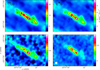 |
Fig. 1. Integrated intensity images of the J = 1−0 transitions of all the CO isotopologues targeted in this work. Line emission is integrated in the velocity range 50−450 km s−1. The common beam size of 3″ (∼50 pc) is shown as a white circle in the bottom left corner of the 13C18O map. The emission of 13C18O is contaminated at the higher velocities in some positions as discussed in Sect. 3.2.1 and shown in Fig. 4. This contamination results in the brighter 13C18O region at position 7 differing from the brightest spot from the other isotopologues approximately at position 9. Marked positions numbered 1 to 14 indicate those selected for spectra extraction and analysis (Sect. 3.2). Nominal positions of the single dish spectra from the literature used for comparison are labelled SD A and B (Sect. 3.1.1). |
Observations of the quasars J0006−0623 and J0038−2459 were performed for bandpass and complex gain calibration, respectively. Absolute flux calibration used observations of Neptune and the quasar J0038−2459. Based on the fluxes derived for the bandpass and gain calibrators between the different dates, we conservatively estimate an uncertainty < 10% between the two frequency set-ups.
Calibration and imaging was performed in CASA version 4.7.2 (McMullin et al. 2007). The continuum emission was subtracted from the visibilities (with the CASA task uvcontsub) using line free channels.
With similar ranges of baseline coverage, the resulting synthesized beams differ only by ∼5% between the two set-ups. Imaging after cleaning was performed with a common circular synthesized beam of 3″ (full width at half maximum; FWHM) for the sake of accurate comparison of flux densities between transitions. This angular resolution is equivalent to ∼50 pc at the distance of NGC 253.
Final data cubes of the individual transitions were smoothed to a common 10 km s−1 velocity resolution. The achieved rms sensitivities in the velocity smoothed cubes were ∼1.5 and ∼5 mJy beam−1, equivalent to ∼19 and ∼62 mK, for the first and second tuning, respectively.
3. Results
3.1. Integrated flux density maps
All targeted CO isotopologues were detected at high signal to noise ratio over the whole CMZ in NGC 253. In Fig. 1 we show the integrated flux density maps of the J = 1−0 transition of all four CO isotopologues. The map of C17O in Fig. 1 at 3″ is similar to that presented by Meier et al. (2015), but the higher spatial resolution allows for resolving the individual GMC complexes in the very central region.
Apart from the difference in line intensities (and therefore also signal to noise ratios), all four isotopologues show a consistent distribution, except for 13C18O which differs on the position of the brighter emission. This is not due to the intrinsic distribution of 13C18O but to the contamination by other species (Sect. 3.2.1). We tried to generate the 13C18O integrated map with a mask per channel based on the emission extent observed in 13CO. Unfortunately, the closeness of the emission of the molecular contaminant at just ∼23 km s−1 (Sect. 3.2.1) from the 13C18O transition made the de-blending impossible in the integrated map. Thus, we preferred to show and use the raw integrated map in the selected velocity range with this limitation in mind when interpreting the map ratios (Sect. 3.1.2).
Carbon and oxygen isotopic ratios can be estimated using the ratio of the carbon monoxide isotopologues as a proxy (Sect. 3.1.2). However, because of the mentioned contamination of the 13C18O emission, a more accurate measurement can be derived from precise modelling and de-blending of its emission from spectra extracted on selected positions (Sect. 3.2).
3.1.1. Spatial filtering
Despite using one of the most compact configurations of the ALMA 12 m array for the sake of achieving a very low brightness temperature sensitivity (Sect. 2), we still expect that a fraction of the flux is filtered out because of our lack of zero spacing observations.
To evaluate the missing flux due to spatial filtering, we reconstructed our ALMA primary beam corrected cubes with a ∼23″ beam, equivalent to that of the IRAM 30 m telescope at the frequency of the CO isotopologues J = 1−0 transitions. We extracted the smoothed spectra at the same positions as those from the single dish observations. These positions (indicated in Fig. 1, upper right panel) are SD A, at  ,
,  , to match the position of the spectra of the four observed isotopologues by Aladro et al. (2015), and SD B,
  ,
,  , to match the position of the 13C18O profile reported by Martín et al. (2010). Extracted spectra on the smoothed cubes are shown in Fig. 2 as grey histograms.
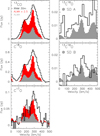 |
Fig. 2. Spectra measured with the IRAM 30 m telescope (Aladro et al. 2015) and the ALMA observations presented in this work. ALMA spectra were extracted at the same positions as the single-dish observations from the data cubes smoothed to 23″ resolution. For 13CO, C18O, and C17O, the ALMA data are shown both with their actual flux (grey histogram) and multiplied by 2.5 (red histogram) for comparison with the single dish line profiles (black line). For 13C18O, we show the profiles in both SD A and SD B positions in Fig. 1, for comparison with the single dish data from Aladro et al. (2015) and Martín et al. (2010), respectively. See text in Sect. 3.1.1 for details. |
Based on our smoothed data cubes we could verify that the published 13C18O integrated flux by Martín et al. (2010; position SD B) would have been 25% brighter if measured towards the position from Aladro et al. (2015; position SD A), which is closer to the galaxy centre. This fact may have an impact in the 12C/13C ratio reported by Martín et al. (2010) as discussed in Sect. 4.2. Moreover, the limited pointing accuracy of the single dish observations may also introduce some uncertainties when comparing different datasets.
The IRAM 30 m single dish spectra1, shown in Fig. 2 in black lines, have been converted to flux density units with a factor of S/TMB = 5 Jy K−1. Additionally, for 13CO, C18O, and C17O, we plot the ALMA spectra (grey histograms) as extracted from the corresponding position in our 23″ smoothed cubes, and also multiplied by a factor of 2.5 (shown in red) for the sake of line shape comparison with the single dish data.
We find that, integrated over the velocity range 40−450 km s−1, only ∼28%, 26%, and 29% of the 13CO, C18O, and C17O single dish flux is recovered by our ALMA data, respectively. These values are very similar and hint at similar spatial distributions as already pointed out in Sect. 3.1 based on the maps in Fig. 1. However, this is around a factor of 2 lower than the flux recovery of 60% reported for C17O by Meier et al. (2015). Such a difference is due to the different single dish integrated flux reported by Henkel et al. (2014; 1.68 ± 0.15 K km s−1) that Meier et al. (2015) used as a reference and the factor of 2 higher value from Aladro et al. (2015; 3.15 ± 0.14 K km s−1) we use in this paper. The different single dish fluxes are due to different observed pointing positions. This is reflected by the narrower line width derived by Henkel et al. (2014), mainly targeting the southwestern part of the central ridge, as compared to that by Aladro et al. (2015). When using the same single dish reference, both Meier et al. (2015) and this work recover the same fluxes. We consider our missing flux estimates more robust since they are derived from smoothed data at the same resolution and position as the single dish data. Meier et al. (2015) reported scales sampled up to 18″ (90th percentile), similar to our larger recoverable scales (Sect. 2), which points to significant amounts of gas at larger scales.
For 13C18O, the recovered flux measured is ∼60% and ∼45% for the Martín et al. (2010) and Aladro et al. (2015) positions, respectively. If we consider velocities only up to 350 km s−1 to reduce the effect of line contamination at the higher velocities (Sect. 3.2.1), the recovered flux yields similar values of ∼55% and ∼45%, respectively. Although, the longer integration at this frequency set-up might result in a better inner-UV coverage, the difference in the recovered flux compared to the other isotopologues can be attributed to: i) significantly varying spatial distribution of 13C18O, which, in principle, we would not expect to be so different from the other rare isotopologues; ii) a higher degree of compactness of the emission of the molecular contaminant (Sect. 3.2.1), which contributes to the measured integrated emission; and more importantly, iii) to the lower signal to noise of this spectral profile affected by both a larger absolute flux uncertainty due to the noise and the extra uncertainty due to the baseline subtraction performed on the single dish spectra (see Fig. 2).
These results point to the uncertainties inherent to single dish observations. In that sense, as pointed out by Meier et al. (2015), the interferometric observations may provide us with a more homogeneous look at the isotopic ratios since we are filtering out approximately the same extended emission in all transitions and therefore we are obtaining information from the same spatial scales. This is also evidenced by the similar line widths from all of our observed line profiles (e.g., in Fig. 2). As mentioned above and followed up in Sect. 4.2, this issue poses some questions regarding the accuracy and interpretation of results obtained from low resolution and non-simultaneous heterogeneous observations.
Figure 2 also shows that should 13C18O be affected by a similar flux filtering as the other isotopologues, assuming a correct baseline subtraction, it should have potentially been detected at higher signal to noise ratio in the IRAM 30 m single dish data by both Martín et al. (2010) and Aladro et al. (2015).
3.1.2. Line ratio maps
In Fig. 3 we show the integrated flux density ratio maps for the relevant pairs of transitions. These ratios have been calculated for pixels where the signal in the integrated maps in the 50−450 km s−1 range is > 1σ, which is > 30 mJy beam−1 km s−1 in 13CO, C18O, and C17O, and > 9.5 mJy beam−1 km s−1 for 13C18O. The uncertainty in these ratio maps is described in Appendix A. The first central C18O contour fulfilling that criterion is shown in both Figs. 3 and A.1, and is considered to be the region of relevance for these ratios. Outside this area, although there is emission above the thresholds, we cannot ensure these are not residuals from the cleaning process.
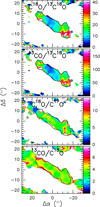 |
Fig. 3. Integrated flux density ratio maps derived from the maps shown in Fig. 1. Only the ratios discussed in the paper are shown. The black contour is the central 1σ level of C18O, used to derive ratio averages within the maps. See Sect. 3.1.2 for details. |
The average and standard deviation within this region with different weighting schemes are shown in Table 1 for each line ratio. The colour scale in Fig. 3 was set from 0 to the unweighted average plus twice the standard deviation. On such a colour scale, the C18O/13C18O ratios appear to be very similar to those of 13CO/13C18O (upper two panels of Fig. 3), indicating a rather constant 13CO/C18O line intensity ratio as can also be seen in the lowest panel of Fig. 3. The C18O/13C18O and 13CO/13C18O ratios appear to show a gradient from the inner region towards the outskirts of the CMZ where some clumps show very high ratios. We note that the decrease of the ratio towards the centre (bluish regions in the upper two panels of Fig. 3) is caused by the increased line contamination in 13C18O as seen in Fig. 1. Thus, C18O/13C18O and 13CO/13C18O ratio maps as well as their derived averages in Table 1 need to be considered with caution in this region as discussed in Sect. 4.1. C18O/C17O and 13CO/C18O appear somewhat smoother, and indeed their relative dispersion in Table 1 are lower than in the other ratios.
Averaged derived isotopic ratios in NGC 253.
3.2. Spectral analysis at selected positions
The positions studied in this work were selected by visually inspecting all the velocity channels in the C18O data cube where individual flux density maxima were identified. The coordinates of the positions identified are listed in Table 2. C18O was selected for this task because it is bright while not affected by the effects of large optical depths, potentially affecting the brighter 13CO, across the whole CMZ. The velocity structure and peak positions are similar for all isotopologues so the position selection is not biased towards 18O enhanced regions. This selection was not based on the previously identified GMC locations from existing high resolution studies of multi-molecular studies of NGC 253 (see Appendix B) since the purpose of this selection was to identify the maxima in our maps to enhance the detectability of the fainter isotopologues.
Fitted parameters to the observed spectra
The integrated map of 13CO in Fig. 1 shows the location of these positions. Table 2 also lists the projected galactocentric distance of each position referred to the bright compact radio source at  ,
,  (Turner & Ho 1985; Ulvestad & Antonucci 1997) assuming a distance of 3.5 Mpc to NGC 253. This distance is projected on the plane of the sky (i.e. not corrected for inclination) and may differ from the actual galactocentric distance, also among velocity components within a given position. Some pairs of positions are very close in projected distance (i.e. positions 6 and 7) but they correspond to the maximum flux densities of two distinct velocity components identified around those positions.
3.2.1. 13C18O line contamination
Martín et al. (2010) identified the contribution of the H2CS 31, 2−21, 1 transition at 104.616 GHz to the 13C18O line profile. The detection of H2CS is actually confirmed by the detection within our observed bands of the 30, 3−20, 2 line at 103.040 GHz with the expected relative flux density.
However, in our high sensitivity data, we also identify two closer features to the 13C18O (1−0) transition, both emitting at lower frequencies (higher velocities). This is particularly obvious in the positions 6 and 7 in Table 2 as shown in Fig. 4 for position 6. As seen in that Figure, the observed profile is not similar to that of 13CO, shown at a scaled down intensity for reference. The line shapes of C17O and C18O, however, match that of 13CO. We note that these two positions are the most affected by this contamination.
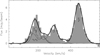 |
Fig. 4. Spectra extracted at position 6 in Table 2. The grey filled histogram shows the spectrum around the 13C18O transition and the velocity scale refers to its rest frequency. The thick curve shows the overall fitted profile to the observations, while the thinner curves show the profiles of 13C18O, as well as the identified emission of the hyperfine structure of C4H (see Sect. 3.2.1 for details) and the line of H2CS. The empty histogram shows the 13CO profile (divided by 100) at the same position as a reference. |
In order to identify the origin of the emission blended to 13C18O we performed a preliminary fit to the spectra in these two positions using four Gaussian profiles; we note that the final fit in Fig. 4 include more Gaussian profiles to account for the faint velocity components of the contaminants. The velocity of the first two were fixed to those of the two components observed in 13CO, to account for the emission of 13C18O. The other two, accounting for the contaminant emission other than the already identified H2CS line, had the velocity as free parameter but the width was fixed to that of the brighter 13CO component. The features which are blended to 13C18O appear at +23.0 ± 1.3 km s−1, and +129.2 ± 1.4 km s−1 with respect to the velocity of the brightest component of 13C18O, which sets the rest frequencies of the contaminating emission at 104703.3 ± 0.5 MHz, and 104666.3 ± 0.5 MHz, respectively.
The spectral scans towards Sgr B2 and the Orion hot cores by Turner (1989) indeed show an unidentified feature at 104696 MHz but nothing at lower frequencies, while the scan by Belloche et al. (2013) towards Sgr B2(N) shows transitions of CH3OCH3 and c-C2H4O around the frequencies of interest, overlapped with a number of vibrational transitions of C2H3CN. Towards Sgr B2(M), on the other hand, Belloche et al. (2013) detected just faint CH3OCH3 emission around 104.7 GHz. However, based on our LTE synthetic spectrum of CH3OCH3, a number of other transitions of this species should have been detected within our observed bandwidth, but they are not, which implies that CH3OCH3 does not contribute significantly to the observed profile. By using the spectroscopic information in the JPL and CDMS catalogues (Pickett et al. 1998; Müller et al. 2001, 2005) we identified that our estimated frequencies agree well with those of the hyperfine transitions of C4H at 104705 MHz (1111−1010) and 104666 MHz (1112−1011) with upper level energies Eu = 30 K. Just recently, C4H was detected for the first time in NGC 253 by Mangum et al. (2019) who reported higher energy transitions (Eu = 126 K) in higher resolution observations. These are the first extragalactic detections of C4H in emission, only previously reported towards the absorption system PKS 1830−211 (Muller et al. 2011).
Despite the strong blending between 13C18O and the 1111−1010 transitions of C4H (low velocity C4H transition in Fig. 4), we were able to account for the contribution of this transition to the observed spectral feature thanks to the relatively cleaner C4H 1112−1011 transitions (higher velocity C4H transition in Fig. 4). So, when analysing the spectra (Sect. 3.2.2), we considered as many velocity components of C4H as those fitted to 13C18O. To de-blend the emission of 13C18O from that of C4H we proceeded as follows. We fitted simultaneously the velocity components of 13C18O and C4H. For the latter we used only the 1112−1011 transitions (farther from the 13C18O transition and therefore cleaner) to fit to the observed C4H emission. Based on the fit to the 1112−1011 transitions, the contribution of the 1111−1010 lines (strongly blended with 13C18O) was then estimated from the expected relative intensities calculated with the spectroscopic parameters of the C4H transitions involved. 13C18O emission was then fitted after removing the contribution of C4H. In some cases where the fainter velocity components of 13C18O were partially blended to the 1112−1011 C4H transitions, this fitting procedure required to be iterated until the fit to all components converged. We also note that the fainter velocity components are subject to stronger blending uncertainties as illustrated in Fig. 4, resulting in large errors in the fits of both C4H and 13C18O. However, the values in Table 2 can be considered as clean 13C18O column densities compared to the 13C18O integrated intensity map in Fig. 1, where the C4H emission is not removed (Sect. 4.1).
3.2.2. 13C18O LTE analysis
Spectra were extracted at each of the selected positions and modelled under the local thermodynamic equilibrium (LTE) assumption using MADCUBA2 (Martín et al., in prep.). With MADCUBA we fit a synthetic spectrum, calculated from input physical parameters and using the molecular spectroscopic parameters in the JPL and CDMS catalogues, to the observed line profiles. The free input parameters that can be fitted are the column density, excitation temperature, velocity, line width, and source size of each molecular species. Figure 4 shows a sample of the synthetic combined profile overlaid on top of the observed spectrum in one of the positions in this study. The results of the multi-Gaussian-component modelling to all selected positions are shown in Table 2 where the obtained column densities derived for each isotopologue, as well as for C4H, are given. The peak flux densities of the observed CO isotopologues spectral lines, even though it is not a direct fitted parameter since MADCUBA does fit the column density, are also listed in Table 2 for reference.
Since this study is based on a single transition of each CO isotopologue, we need to make a number of assumptions: i) all isotopologues have the same distribution, including velocity profile; ii) they have a common excitation temperature of Tex = 15 K; and iii) the source size is 3″, matching the map resolution. We explain the implications of such assumptions below.
The velocities and widths were fitted to the 13CO profiles, and then set as fixed parameters when fitting the other isotopologues and C4H. This constraint was imposed to ensure consistency in the line profiles fitted, but in any case, letting these parameters free resulted in consistent values within the errors in the cases where the fit was possible both in terms of having enough signal to noise and not being significantly affected by line blending. Thus, fixing the velocity and width was only critical in the spectra with low signal to noise ratios and those of 13C18O where line blending was observed (Sect. 3.2.1).
The excitation temperature was fixed to 15 K based on the rotational temperatures derived from multi-transition studies based on previous spectral scans (Martín et al. 2006) and on preliminary results from the ALMA multi-band spectral scan on NGC 253 (Martín et al., in prep.). Differences in the assumed excitation temperature have a minor impact on the derived column densities. For temperatures of 10 and 20 K, we estimate column densities ∼5% and ∼10% higher, respectively. However this would affect all isotopologues similarly if we assume they share similar excitation conditions, and therefore column density ratios would remain virtually unchanged. For temperatures below 10 K it is not possible to fit the intensity of observed profiles for any combination of column density and source size.
The column density and optical depth of the 13CO transition are directly linked to the assumed source size, therefore these values would both increase under the assumption of a smaller source size. High resolution imaging by Ando et al. (2017) resulted in resolved GMCs of ∼9 pc (0.5″) in size. However, in the case of position 9 in Table 2, the position with the largest measured optical depth (Table 2), we are not able to reproduce the observed flux density for source sizes < 2″ unless significantly increasing the excitation temperature. However as indicated above, multi-transition studies do not point towards such high excitation temperatures. Thus we assume that the observed profiles stem from 2−3″ averaged regions. For a source size of 2″, derived 13CO column densities in Table 2 would be underestimated by up to a factor of 3 in the brightest position 9. However, for all other positions, less affected by optical thickness, 13CO column densities would be underestimated by a factor of ≲2.3. On the other hand, the column density ratios in this study, would be underestimated by up to 40% in position 9 for the ratios involving 13CO, but we enter into the optically thick regime where fitted parameters strongly depend on the assumptions of source size and excitation temperature. For the optically thinner lines of sights and isotopologues, the derived ratios would mostly be unaltered.
Based on the column densities in Table 2, in Table 1 we show the average of the column density ratios and standard deviations calculated with the values obtained from all selected positions. These ratios do not include the positions where only upper limits to the 13C18O were obtained. The averages and standard deviations are calculated: unweighted as a raw value, weighted by the standard deviation of individual measurements to get the average of the ratios measured at higher signal to noise or less blending, and weighted by the optical depth of 13CO as representative of the most massive clouds sampled.
4. Discussion
4.1. Map versus spectra ratios: Optical depth and contamination effects.
From Table 1 we see how the average isotopologue ratios, calculated as the column density ratios derived from the spectral analysis (Sect. 3.2.2) vary little and within the uncertainties when different weighting schemes are used. Although still consistent within the error bars (when unweighted averages are considered), these values from spectral analysis are higher than those measured from the averaging of the maps. These differences can be considered significant since they are both measured with the same dataset. We discuss why these difference can be attributed to a combined effect of both optical depth and line contamination affecting the lines in the measured ratio.
As explained above, 13CO is affected by significant optical depth (Sect. 3.2.2) while 13C18O is contaminated by C4H. Thus, we observe that the optical depth affected ratio 13CO/C18O is 38 ± 6% smaller in the averaged map than from the spectra (considering unweighted values from Table 1). On the other hand, the contamination affected ratio C18O/13C18O is observed to be 22 ± 9% smaller. Subsequently, the 13CO/13C18O ratio, affected by both effects, should differ by approximately the multiplication of both factors, and therefore be 70 ± 40% smaller and, indeed the observed difference between the spectra and map derived average is 90 ± 40%.
This explanation is further supported by the fact that the derived averages diverge even further from those derived with the spectra when weighted by the standard deviation or the signal to noise ratio per pixel. These weightings favour the brighter regions, which are those that are either more opaque and/or more contaminated by C4H.
On the other hand, the C18O/C17O ratio is not expected to be affected by line saturation and we observe that this is the only ratio which is higher in the averaged maps compared to the spectra and which show little variation with the weighted averages from the maps. Therefore, the differences between the values derived from the maps and the spectra can be actually attributed to actual spatial variations. We note that the small variation derived from the weighted average in the C18O/C17O ratio, could still be due to significant optical depth in the C18O emission.
Based on the arguments above we can safely consider that the values derived from the spectra are the most accurate optical depth and contamination corrected values as proxies of the elemental isotopic ratios in NGC 253. While we adopt the σ-weighted ratios from the spectra for the discussion on stellar processing in Sect. 4.4, we use the unweighted values as reference for comparison with previous single dish data in the literature in Sect. 4.2.
4.2. Spatially resolved carbon and oxygen ratios with optically thin tracers
Based on the observations presented in this paper, we can for the first time derive spatially resolved carbon and oxygen isotopic ratios based on the rarer carbon monoxide isotopologues. This is under the assumption that the column density ratio of the molecular isotopologues reflects the actual atomic isotopic ratio.
As seen in Figs. 3 and 5, the measured isotopic ratios vary significantly across the CMZ in NGC 253. Based on the column density values determined from the spectra (Table 2), we observe ratios ranging from 10 to 34 for 12C/13C, 45 to 270 for 16O/18O, and to a lesser extent 2.7 to 8.5 for 18O/17O. Still, on average our high resolution results are about a factor of two below those typically assumed in the nuclei of galaxies (Wilson & Rood 1994; Henkel et al. 1994; Wang et al. 2004).
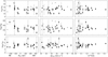 |
Fig. 5. Measured isotopic ratios as a function of galactocentric distance, FWHM of the fitted profile, and optical depth of the 13CO transition. Ratios are calculated based on the column density ratios in Table 2. Lower limits (3σ) to the ratios due to non-detection of 13C18O are represented as open circles. |
As indicated in the introduction the selection of optically thin tracers minimizes the effect of selective photodissociation. However, if 13C18O should be affected by a higher photodissociation rate (Visser et al. 2009), the ratios derived in this paper would be even lower. However, we have no evidence to support such effect globally within the central region of NGC 253.
We put our results in the context of previously determined isotopic ratios towards NGC 253.
4.2.1. 12C/13C
The single dish ratio C18O/13C18O≳60 reported by Martín et al. (2010) differs by a factor of 3 from the ratio reported in this work. We note that the C18O peak temperature reported by Martín et al. (2010) is 75% brighter than that reported by Aladro et al. (2015). Additionally, 13C18O and C18O were observed at different positions, SD B and SD A, respectively. As explained in Sect. 3.1.1, 13C18O could be 25% brighter towards the SD A position. Thus, if these uncertainties align in the same direction, the ratio derived by Martín et al. (2010) could result in a value as low as ≳35, which is closer to the value derived with other tracers (Henkel et al. 2014), but still higher than the value derived in this paper. However, the single dish value from Martín et al. (2010) is uncertain because of the unknown systematic errors resulting from the use of heterogeneous datasets.
The value derived from our optically thin observations is a factor of 2 lower than the ratio typically assumed for galaxies (Wilson & Rood 1994; Henkel et al. 2014) and a factor of 2−4 below the limits based on CCH (Martín et al. 2010), in this case derived from the homogeneous spectral scan dataset by Martín et al. (2006).
As we discuss in Sect. 4.4, this difference may be real and a result of spatially distinct molecular gas component with different degrees of stellar processing.
4.2.2. 16O/18O
The value quoted in the literature (Wilson & Rood 1994) of ∼200 is derived from the 13CO/C18O ratio reported by Sage et al. (1991) in a sample of three galaxies (NGC 253, IC 342, M 82), and multiplied by the assumed 12C/13C ∼ 40 (Henkel et al. 1993). For NGC 253, Sage et al. (1991) reported 13CO/C18O = 4.9 ± 0.5, which is good agreement with the value of 4.5 ± 1.7 derived from our map measurements in Table 2. If we use our derived 12C/13C to multiply the measurement by Sage et al. (1991), we obtain a ratio 16O/18O = 110 ± 30, which is consistent with our optical depth/contamination corrected (Sect. 3.2) measurement of 13CO/13C18O. Thus, the discrepancy between the 16O/18O ratio reported in this work and that of Wilson & Rood (1994) resides on the large scale 12C/13C ratio differing from that measured at high resolution.
4.2.3. 18O/17O
Sage et al. (1991) reported a 18O/17O of 10 ± 2.5 based on C18O/C17O J = 2−1 observations towards NGC 253. The discrepancy can be attributed to the low signal to noise ratio of their single dish data. The higher sensitivity observations by Aladro et al. (2015) of the J = 1−0 yield a ratio of 7.1 ± 0.4, also in good agreement with the map derived value of 6.5 ± 3.7 in Table 1.
4.3. Isotopic ratio variations across the CMZ of NGC 253
Since the ALMA observations allowed us to spatially resolve the CMZ of NGC 253 we explore the variations of isotopic ratios among the individual identified sources across this region.
Within our Galaxy, a clear gradient as a function of the galactocentric distance is observed in the carbon, oxygen and nitrogen isotopic ratios (Gardner & Whiteoak 1979; Henkel et al. 1982; Langer & Penzias 1990; Wilson & Rood 1994; Goto et al. 2003; Milam et al. 2005; Wouterloot et al. 2008; Zhang et al. 2015). The left panels in Fig. 5 show the variation of estimated isotopic ratios as a function of the linear projected distance measured from the assumed galactic centre position (see Sect. 3.2). We do not observe an obvious gradient in our data as a function of galactocentric distance. However, we note that, within the Galaxy, this gradient is observed at distances ranging 3–10 kpc, while our observations in NGC 253 cover the inner ∼300 pc. In fact, considering the dispersion of the observations at a given Galactocentric distance, such gradient, should it continue towards the very central region, might not be distinguished within the central few hundred parsecs of the Galaxy as is the case in NGC 253. Most of these studies present only one observational point towards the Galactic centre ranging 12C/13C = 17 ± 7 (where the error includes the variation of the ratio measured with different molecular tracers used, Langer & Penzias 1990; Milam et al. 2005) with a standard value generally adopted of ∼20 (Wilson & Rood 1994). Moreover, the study by Gardner & Whiteoak (1982) shows that the low ratio of ratio 12C/13C ∼ 15 ± 4, as measured with H2CO, is relatively homogeneously observed across the CMZ and not exclusively from individual sources like Sgr A or Sgr B2. This is similar to the relatively homogeneous ratios observed within the CMZ of NGC 253. Similarly, oxygen ratios show no variations with distance from the centre of NGC 253 within a radius of 300 pc. Similarly, we do not observe obvious gradients in 16O/18O and 18O/17O ratios, with observed ratios within 25% of the average (see Table 1).
In order to further investigate the relative variations of the isotopic ratios among molecular components, we plot the measured ratios as a function of the observed line width. Line width was taken as a proxy of the virial mass of the unresolved clouds because of the lack of an a priori knowledge of their individual sizes. Then central panels in Fig. 5 show no apparent trend with the line width on any of the isotopic ratios.
The right panels in Fig. 5 show the ratio dependency on the measured optical depth of 13CO (13τ) at each position. This optical depth assumes the same source size for all sources. The implications of this assumption have already been discussed in Sect. 3.2 and translate into an uncertainty in the x-axis of this dependency, where points might be displaced by up to a factor of ∼2 towards higher optical depths for some positions. Once again, no obvious trend is observed. However the most uncertain ratios are found towards the weaker molecular components such as those with lower optical depths and therefore column densities; this results in larger error bars and uncertain lower limits in the 12C/13C and 16O/18O owing to the strong blending with C4H (Sect. 3.2.1). This is also reflected in larger uncertainties due to the limited signal to noise ratios in 18O/17O, unaffected by blending.
Additionally, in Fig. 6 we show the variations of the carbon and oxygen isotopic ratios across all the positions selected, where the different velocity components are separated into four colour groups, according to the measured ratios, where also the optical depth of 13CO is coded with the size of the points. Higher granularity in the colour coding does not provide a more accurate picture given the errors in the ratios.
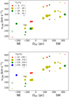 |
Fig. 6. Colour-coded carbon (top panel) and oxygen (bottom panel) isotopic ratios as a function of the distance to the galaxy centre and separated by the measured velocity of each fitted component. Colour-coding ranges were selected to distinguish four quartiles between the minimum and maximum values measured in all components. The size of the points is related to the optical depth of the 13CO. Open symbols represent lower limits. |
In contrast to the situation in our Galactic centre (Fig. 2 in Gardner & Whiteoak 1982), in this work we can assume that all velocity components are located within the CMZ. However our spatial resolution is not high enough to provide an accurate picture of their locations. Higher resolution observations will provide a more accurate picture of the isotopic distribution.
We observe an overall homogeneity of the measured isotopic ratios where most of the gas is around the averaged reported values. Only a few low column density velocity components show ratios significantly above or below the average (blue and red, respectively, in Fig. 6).
4.4. Stellar processed gas in the galactic centre of NGC 253
The relatively large 12C/13C ratio observed in NGC 253 (and other starbursts galaxies) as compared to that in the Galactic centre has been claimed as the result of infalling unprocessed material into the central region. Such accretion has also been claimed towards the CMZ of the Milky Way through the study of isotopic enrichment (Riquelme et al. 2010). Our results show that at high resolution the degree of stellar processing of the molecular gas in the CMZ of NGC 253, as measured by carbon monoxide isotopologues, appears to be similar to that in the CMZ of the Galaxy.
Our 12C/13C ratio of 21 ± 6 is well in agreement with the value of 24 ± 1 in the Galactic centre, measured with the sames isotopologue transitions of CO (Langer & Penzias 1990), while the 16O/18O ratio of 130 ± 40 is about half of the 250 measured there (Wilson & Rood 1994). However, the value in NGC 253 would result in a good agreement if we extrapolate the galactocentric trend observed across the large scale disc of the Galaxy (Fig. 2 in Wilson & Rood 1994). Similarly, the 18O/17O ratio of 4.5 ± 0.8 is about 50% larger than the measurements by Zhang et al. (2015) towards our Galactic centre. The smaller 16O/18O and larger 18O/17O observed ratios may point towards an actual enhancement of 18O as compared to the CMZ of the Milky Way. This might be attributed to the fast enhancement of 18O by massive stars, while 13C and 17O are more slowly injected by low- and intermediate-mass stars (Zhang et al. 2018). Indeed, Zhang et al. (2015) found a difference in the 18O/17O ratio of the Galactic centre to the molecular clouds in the disc, which implies differences in the gas phase injection of these isotopes.
Our result at high resolution implies that the low resolution ratios measured with single dish observations actually reflect an average global value that may include two well separated molecular components: one significantly processed by the past star formation in the nuclear region and a less processed component likely infalling from the outer disc that will presumably be feeding the future star formation in the region.
In this scenario, the recent accurate optical depth corrected 12C/13C measurement of ∼40 based on CN observations by Henkel et al. (2014) would actually be the average of the processed material in the central region (12C/13C ∼ 20) plus a molecular component with a higher 12C/13C ratio. If we consider the recovered fluxed estimated in Sect. 3.1.1, the filtered out molecular component would correspond to ∼70% of the 13CO single dish emission, as well as 40−55% of that of 13C18O. This yields isotopic ratios for the filtered component of 12C/13C ∼ 50−70, in order to explain the global averaged single dish carbon isotopic ratio. This extended molecular component might be actually that traced by CCH (Martín et al. 2010), where ratios > 56 and > 81 were estimated based on the non-detection of 13CCH, and the stacked spectra of 13CCH+C13CH, respectively. In fact, the observation of CN obtained as part of the ALCHEMI line survey towards NGC 253 (Martín et al., in prep.) show an optical depth well in excess of the τ ∼ 0.2−0.5 obtained by single dish data (Henkel et al. 2014), which would further support the fact that single dish data are indeed the result of the averaging of an optically thin extended molecular component plus a compact optically thick one. A similar calculation cannot be estimated for the extended 16O/18O ratio since the single dish global value is actually derived through assumptions on the 12C/13C ratio as explained in Sect. 4.2.
While large scale extragalactic unresolved observations might still make use of commonly assumed single dish derived ratios, high resolution observations may need to consider the multicomponent nature of the molecular clouds in the central region of galaxies. As an example, we note that the HCN/H13CN and HCO+/H13CO+ line ratios ranging 10−15 obtained at 2″ resolution (Meier et al. 2015) are actually close to the 12C/13C isotopic ration derived in this paper. Thus their derived optical depths of τ ∼ 5−8 for HCN and HCO+ would actually be significantly overestimated. If we recalculate the optical depths for these two dense gas traces assuming our derived 12C/13C ∼ 21, it results in moderate optical depths of τ ∼ 0.7−1.7.
Our results also shed some doubts on the feasibility of inferring the history of stellar nucleosynthesis and the characteristics of the IMF in galaxies based on global isotopic ratios (Romano et al. 2017). Actually the molecular gas affected by the stellar nucleosynthesis in the central region might be masked or diluted by the infalling of gas from less processed regions, as it appears to be the case in NGC 253, or as result of galactic interactions. Zhang et al. (2018) recently reported a potential trend of the 13CO/C18O line ratio as a function of the infrared luminosity in a sample of extragalactic sources. This trend is claimed to be linked to the stellar IMF. In that scenario, the lowest ratios of ∼1 would be the result of a top-heavy stellar IMF. However, once again this is based on a single ratio at low spatial resolution, while our study shows the significant difference between the direct measurements from the maps and the optical depth corrected values towards the selected positions (Sect. 3.2).
5. Conclusions
The main results from the observations of the rarer isotopologues of carbon monoxide are the following. For the first time we present unambiguous and spatially resolved detections of the double substitution of carbon monoxide 13C18O in the extragalactic ISM of the starburst NGC 253. Carbon and oxygen isotopologue ratios have been derived with optically thin tracers at high spatial resolution resulting in lower values than previously obtained with single dish low resolution data. Our derived ratios take into account and correct the contamination of 13C18O by C4H and the moderate optical thickness of 13CO. The deduced 12C/13C ∼ 21 agrees with the value measured towards the centre of the Milky Way, which can be understood in terms of a similar degree of nuclear processing from stellar nucleosynthesis. Both 16O/18O ∼ 130 and 18O/17O ∼ 4.5 are well below and above those measured in the Galactic centre, respectively, which points out to a 18O enhancement by massive stars and a slower injection of 13C by low- and intermediate-mass stars. Differences from the ratios observed with single dish telescopes appear to present evidence of a multicomponent scenario with molecular gas highly processed in the central region of NGC 253 and unprocessed gas claimed to be infalling from the outer regions of the galaxy. No obvious gradients are found as a function of the distance to the centre out to galactocentric radii of ∼300 pc.
Acknowledgments
SM wants to thank the valuable discussions with V. Rivilla, J. Martín-Pintado, and Laura Colzi on the results presented in this paper. KS was supported by the MOST grant 107-2119-M-001-022. This paper makes use of the following ALMA data: ADS/JAO.ALMA#2016.1.00292.S. ALMA is a partnership of ESO (representing its member states), NSF (USA) and NINS (Japan), together with NRC (Canada), MOST and ASIAA (Taiwan), and KASI (Republic of Korea), in cooperation with the Republic of Chile. The Joint ALMA Observatory is operated by ESO, AUI/NRAO and NAOJ.
References
- Aladro, R., Martín, S., Riquelme, D., et al. 2015, A&A, 579, A101 [NASA ADS] [CrossRef] [EDP Sciences] [Google Scholar]
- Ando, R., Nakanishi, K., Kohno, K., et al. 2017, ApJ, 849, 81 [NASA ADS] [CrossRef] [Google Scholar]
- Belloche, A., Müller, H. S. P., Menten, K. M., Schilke, P., & Comito, C. 2013, A&A, 559, A47 [NASA ADS] [CrossRef] [EDP Sciences] [Google Scholar]
- Chiappini, C., Ekström, S., Meynet, G., et al. 2008, A&A, 479, L9 [NASA ADS] [CrossRef] [EDP Sciences] [Google Scholar]
- Gardner, F. F., & Whiteoak, J. B. 1979, MNRAS, 188, 331 [NASA ADS] [CrossRef] [Google Scholar]
- Gardner, F. F., & Whiteoak, J. B. 1982, MNRAS, 199, 23P [NASA ADS] [CrossRef] [Google Scholar]
- Goto, M., Usuda, T., Takato, N., et al. 2003, ApJ, 598, 1038 [NASA ADS] [CrossRef] [Google Scholar]
- Henkel, C., & Mauersberger, R. 1993, A&A, 274, 730 [NASA ADS] [Google Scholar]
- Henkel, C., Wilson, T. L., & Bieging, J. 1982, A&A, 109, 344 [NASA ADS] [Google Scholar]
- Henkel, C., Mauersberger, R., Wiklind, T., et al. 1993, A&A, 268, L17 [NASA ADS] [Google Scholar]
- Henkel, C., Wilson, T. L., Langer, N., Chin, Y. N., & Mauersberger, R. 1994, in The Structure and Content of Molecular Clouds, eds. T. L. Wilson, & K. J. Johnston, Lect. Notes Phys. (Berlin: Springer Verlag), 439, 72 [Google Scholar]
- Henkel, C., Asiri, H., Ao, Y., et al. 2014, A&A, 565, A3 [NASA ADS] [CrossRef] [EDP Sciences] [Google Scholar]
- Ikeda, M., Hirota, T., & Yamamoto, S. 2002, ApJ, 575, 250 [NASA ADS] [CrossRef] [Google Scholar]
- Jiménez-Donaire, M. J., Cormier, D., Bigiel, F., et al. 2017, ApJ, 836, L29 [NASA ADS] [CrossRef] [Google Scholar]
- Karakas, A. I., & Lattanzio, J. C. 2014, PASA, 31, e030 [NASA ADS] [CrossRef] [Google Scholar]
- Krips, M., Martín, S., Peck, A. B., et al. 2016, ApJ, 821, 112 [NASA ADS] [CrossRef] [Google Scholar]
- Langer, W. D., & Penzias, A. A. 1990, ApJ, 357, 477 [NASA ADS] [CrossRef] [Google Scholar]
- Langer, W. D., Graedel, T. E., Frerking, M. A., & Armentrout, P. B. 1984, ApJ, 277, 581 [NASA ADS] [CrossRef] [Google Scholar]
- Leroy, A. K., Bolatto, A. D., Ostriker, E. C., et al. 2015, ApJ, 801, 25 [NASA ADS] [CrossRef] [Google Scholar]
- Limongi, M., & Chieffi, A. 2018, ApJS, 237, 13 [NASA ADS] [CrossRef] [Google Scholar]
- Loison, J. C., Wakelam, V., Gratier, P., et al. 2019, MNRAS, 485, 5777 [NASA ADS] [CrossRef] [Google Scholar]
- Mangum, J. G., Darling, J., Henkel, C., et al. 2013, ApJ, 779, 33 [NASA ADS] [CrossRef] [Google Scholar]
- Mangum, J. G., Ginsburg, A. G., Henkel, C., et al. 2019, ApJ, 871, 170 [NASA ADS] [CrossRef] [Google Scholar]
- Martín, S., Martín-Pintado, J., Mauersberger, R., Henkel, C., & García-Burillo, S. 2005, ApJ, 620, 210 [NASA ADS] [CrossRef] [Google Scholar]
- Martín, S., Mauersberger, R., Martín-Pintado, J., Henkel, C., & García-Burillo, S. 2006, ApJS, 164, 450 [NASA ADS] [CrossRef] [Google Scholar]
- Martín, S., Aladro, R., Martín-Pintado, J., & Mauersberger, R. 2010, A&A, 522, A62 [NASA ADS] [CrossRef] [EDP Sciences] [Google Scholar]
- McMullin, J. P., Waters, B., Schiebel, D., Young, W., & Golap, K. 2007, in Astronomical Data Analysis Software and Systems XVI, eds. R. A. Shaw, F. Hill, & D. J. Bell, ASP Conf. Ser., 376, 127 [Google Scholar]
- Meier, D. S., & Turner, J. L. 2001, ApJ, 551, 687 [NASA ADS] [CrossRef] [Google Scholar]
- Meier, D. S., Walter, F., Bolatto, A. D., et al. 2015, ApJ, 801, 63 [NASA ADS] [CrossRef] [Google Scholar]
- Meyer, B. S. 1994, ARA&A, 32, 153 [NASA ADS] [CrossRef] [Google Scholar]
- Milam, S. N., Savage, C., Brewster, M. A., Ziurys, L. M., & Wyckoff, S. 2005, ApJ, 634, 1126 [NASA ADS] [CrossRef] [Google Scholar]
- Mouhcine, M., Ferguson, H. C., Rich, R. M., Brown, T. M., & Smith, T. E. 2005, ApJ, 633, 810 [NASA ADS] [CrossRef] [Google Scholar]
- Müller, H. S. P., Thorwirth, S., Roth, D. A., & Winnewisser, G. 2001, A&A, 370, L49 [NASA ADS] [CrossRef] [EDP Sciences] [Google Scholar]
- Müller, H. S. P., Schlöder, F., Stutzki, J., & Winnewisser, G. 2005, J. Mol. Struct., 742, 215 [NASA ADS] [CrossRef] [Google Scholar]
- Muller, S., Beelen, A., Guélin, M., et al. 2011, A&A, 535, A103 [NASA ADS] [CrossRef] [EDP Sciences] [Google Scholar]
- Ott, J., Weiss, A., Henkel, C., & Walter, F. 2005, ApJ, 629, 767 [NASA ADS] [CrossRef] [Google Scholar]
- Pickett, H. M., Poynter, I. R. L., Cohen, E. A., et al. 1998, J. Quant. Spectr. Rad. Transf., 60, 883 [NASA ADS] [CrossRef] [Google Scholar]
- Rekola, R., Richer, M. G., McCall, M. L., et al. 2005, MNRAS, 361, 330 [NASA ADS] [CrossRef] [Google Scholar]
- Riquelme, D., Amo-Baladrón, M. A., Martín-Pintado, J., et al. 2010, A&A, 523, A51 [NASA ADS] [CrossRef] [EDP Sciences] [Google Scholar]
- Röllig, M., & Ossenkopf, V. 2013, A&A, 550, A56 [NASA ADS] [CrossRef] [EDP Sciences] [Google Scholar]
- Romano, D., Matteucci, F., Zhang, Z.-Y., Papadopoulos, P. P., & Ivison, R. J. 2017, MNRAS, 470, 401 [NASA ADS] [CrossRef] [Google Scholar]
- Roueff, E., Loison, J. C., & Hickson, K. M. 2015, A&A, 576, A99 [NASA ADS] [CrossRef] [EDP Sciences] [Google Scholar]
- Sage, L. J., Henkel, C., & Mauersberger, R. 1991, A&A, 249, 31 [NASA ADS] [Google Scholar]
- Sakamoto, K., Mao, R.-Q., Matsushita, S., et al. 2011, ApJ, 735, 19 [NASA ADS] [CrossRef] [Google Scholar]
- Szűcs, L., Glover, S. C. O., & Klessen, R. S. 2014, MNRAS, 445, 4055 [NASA ADS] [CrossRef] [MathSciNet] [Google Scholar]
- Turner, B. E. 1989, ApJS, 70, 539 [NASA ADS] [CrossRef] [Google Scholar]
- Turner, J. L., & Ho, P. T. P. 1985, ApJ, 299, L77 [NASA ADS] [CrossRef] [Google Scholar]
- Ulvestad, J. S., & Antonucci, R. R. J. 1997, ApJ, 488, 621 [NASA ADS] [CrossRef] [Google Scholar]
- Visser, R., van Dishoeck, E. F., & Black, J. H. 2009, A&A, 503, 323 [NASA ADS] [CrossRef] [EDP Sciences] [Google Scholar]
- Wallström, S. H. J., Muller, S., & Guélin, M. 2016, A&A, 595, A96 [NASA ADS] [CrossRef] [EDP Sciences] [Google Scholar]
- Walter, F., Bolatto, A. D., Leroy, A. K., et al. 2017, ApJ, 835, 265 [NASA ADS] [CrossRef] [Google Scholar]
- Wang, M., Henkel, C., Chin, Y., et al. 2004, A&A, 422, 883 [NASA ADS] [CrossRef] [EDP Sciences] [Google Scholar]
- Watson, W. D. 1977, in CNO Isotopes in Astrophysics, ed. J. Audouze, Astrophys. Space Sci. Lib., 67, 105 [NASA ADS] [CrossRef] [Google Scholar]
- Wilson, T. L., & Matteucci, F. 1992, A&ARv, 4, 1 [NASA ADS] [CrossRef] [Google Scholar]
- Wilson, T. L., & Rood, R. 1994, ARA&A, 32, 191 [NASA ADS] [CrossRef] [Google Scholar]
- Wouterloot, J. G. A., Henkel, C., Brand, J., & Davis, G. R. 2008, A&A, 487, 237 [NASA ADS] [CrossRef] [EDP Sciences] [Google Scholar]
- Zhang, J. S., Sun, L. L., Riquelme, D., et al. 2015, ApJS, 219, 28 [NASA ADS] [CrossRef] [Google Scholar]
- Zhang, Z.-Y., Romano, D., Ivison, R. J., Papadopoulos, P. P., & Matteucci, F. 2018, Nature, 558, 260 [NASA ADS] [CrossRef] [Google Scholar]
Appendix A: Error and signal to noise in line ratio maps
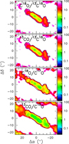 |
Fig. A.1. Accuracy of the ratio maps shown in Fig. 3 in percentage as defined in Eq. (A.1). The black contour is similar to that in Fig. 3. |
While Fig. 1 shows the ratio R = M1/M2 between the corresponding maps M1 and M2, Fig. A.1 gives the ratio of the propagated error of the ratio map to the ratio map in percentage as
 (A.1)
(A.1)
where we observe how the central region, as expected, has errors of ∼1% rising to a few 10% towards the edge of the region considered (see Sect. 3.1.2).
Figure A.2, on the other hand, shows the signal to noise ratio per pixel of the ratio maps (R/σR) as a function of the ratio. The effect of line contamination by C4H (Sect. 3.2.1) in the C18O/13C18O and 13CO/13C18O is clearly seen as the double peak structure and a broad tail both at high signal to noise as a result of the different distributions between the CO isotopologues and C4H. This is different from what is observed in the C18O/C17O and 13CO/C18O ratios which show a single peaked distribution. The effect of the significant 13CO optical depth is evidenced by the 13CO/C18O distribution being skewed towards lower values, which is different from what we observe in the optically thin ratio C18O/C17O more symmetrical distribution. Similarly the two high signal to noise components in 13CO/13C18O are also pushed together by the effect of optical depth. See Sect. 4.1 for further discussion of both optical depth and line contamination effects on ratio maps based on the differences observed with the ratios from spectral analysis.
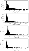 |
Fig. A.2. Signal to noise ratios per pixel in the ratio maps of Fig. 3 as a function of the line ratio. |
Appendix B: Selected positions: Comparison to other works
Positions in this work are based on observed maxima in the C18O channel maps (see Sect. 3.2) and not from those in previous high resolution studies (Sakamoto et al. 2011; Meier et al. 2015; Ando et al. 2017; Leroy et al. 2015; Walter et al. 2017). Figure B.1 shows the positions selected in this paper compared to those by Meier et al. (2015) aiming at sampling different regions in NGC 253 CMZ, those of Sakamoto et al. (2011) identifying the brightest spots in the integrated intensity maps, and those of the high resolution study by Ando et al. (2017) identifying the peak continuum sources in the very inner region. The different angular resolutions of these studies in the literature are also shown in this Fig. B.1.
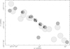 |
Fig. B.1. Location of the positions analysed in this paper (3″, light grey circles), compared to the positions from Meier et al. (2015; 2″, grey circles), Sakamoto et al. (2011; 1.1″, dark grey circles), and Ando et al. (2017; ∼0.37″, black dots). The size of the circles represent the resolution of the observations in these studies. |
All Tables
All Figures
|
Fig. 1. Integrated intensity images of the J = 1−0 transitions of all the CO isotopologues targeted in this work. Line emission is integrated in the velocity range 50−450 km s−1. The common beam size of 3″ (∼50 pc) is shown as a white circle in the bottom left corner of the 13C18O map. The emission of 13C18O is contaminated at the higher velocities in some positions as discussed in Sect. 3.2.1 and shown in Fig. 4. This contamination results in the brighter 13C18O region at position 7 differing from the brightest spot from the other isotopologues approximately at position 9. Marked positions numbered 1 to 14 indicate those selected for spectra extraction and analysis (Sect. 3.2). Nominal positions of the single dish spectra from the literature used for comparison are labelled SD A and B (Sect. 3.1.1). |
| In the text | |
|
Fig. 2. Spectra measured with the IRAM 30 m telescope (Aladro et al. 2015) and the ALMA observations presented in this work. ALMA spectra were extracted at the same positions as the single-dish observations from the data cubes smoothed to 23″ resolution. For 13CO, C18O, and C17O, the ALMA data are shown both with their actual flux (grey histogram) and multiplied by 2.5 (red histogram) for comparison with the single dish line profiles (black line). For 13C18O, we show the profiles in both SD A and SD B positions in Fig. 1, for comparison with the single dish data from Aladro et al. (2015) and Martín et al. (2010), respectively. See text in Sect. 3.1.1 for details. |
| In the text | |
|
Fig. 3. Integrated flux density ratio maps derived from the maps shown in Fig. 1. Only the ratios discussed in the paper are shown. The black contour is the central 1σ level of C18O, used to derive ratio averages within the maps. See Sect. 3.1.2 for details. |
| In the text | |
|
Fig. 4. Spectra extracted at position 6 in Table 2. The grey filled histogram shows the spectrum around the 13C18O transition and the velocity scale refers to its rest frequency. The thick curve shows the overall fitted profile to the observations, while the thinner curves show the profiles of 13C18O, as well as the identified emission of the hyperfine structure of C4H (see Sect. 3.2.1 for details) and the line of H2CS. The empty histogram shows the 13CO profile (divided by 100) at the same position as a reference. |
| In the text | |
|
Fig. 5. Measured isotopic ratios as a function of galactocentric distance, FWHM of the fitted profile, and optical depth of the 13CO transition. Ratios are calculated based on the column density ratios in Table 2. Lower limits (3σ) to the ratios due to non-detection of 13C18O are represented as open circles. |
| In the text | |
|
Fig. 6. Colour-coded carbon (top panel) and oxygen (bottom panel) isotopic ratios as a function of the distance to the galaxy centre and separated by the measured velocity of each fitted component. Colour-coding ranges were selected to distinguish four quartiles between the minimum and maximum values measured in all components. The size of the points is related to the optical depth of the 13CO. Open symbols represent lower limits. |
| In the text | |
|
Fig. A.1. Accuracy of the ratio maps shown in Fig. 3 in percentage as defined in Eq. (A.1). The black contour is similar to that in Fig. 3. |
| In the text | |
|
Fig. A.2. Signal to noise ratios per pixel in the ratio maps of Fig. 3 as a function of the line ratio. |
| In the text | |
|
Fig. B.1. Location of the positions analysed in this paper (3″, light grey circles), compared to the positions from Meier et al. (2015; 2″, grey circles), Sakamoto et al. (2011; 1.1″, dark grey circles), and Ando et al. (2017; ∼0.37″, black dots). The size of the circles represent the resolution of the observations in these studies. |
| In the text | |
Current usage metrics show cumulative count of Article Views (full-text article views including HTML views, PDF and ePub downloads, according to the available data) and Abstracts Views on Vision4Press platform.
Data correspond to usage on the plateform after 2015. The current usage metrics is available 48-96 hours after online publication and is updated daily on week days.
Initial download of the metrics may take a while.