| Issue |
A&A
Volume 624, April 2019
|
|
|---|---|---|
| Article Number | A11 | |
| Number of page(s) | 17 | |
| Section | Extragalactic astronomy | |
| DOI | https://doi.org/10.1051/0004-6361/201834871 | |
| Published online | 01 April 2019 | |
Satellite dwarf galaxies: stripped but not quenched
1
Laboratoire d’Astrophysique, Ecole Polytechnique Fédérale de Lausanne (EPFL), 1290 Sauvergny, Switzerland
e-mail: This email address is being protected from spambots. You need JavaScript enabled to view it.
2
CNRS UMR 8111, GEPI, Observatoire de Paris, Université PSL, 92125 Meudon Cedex, France
Received:
14
December
2018
Accepted:
31
January
2019
Abstract
In the Local Group, quenched gas-poor dwarfs galaxies are most often found close to the Milky Way and Andromeda, while star forming gas-rich ones are located at greater distances. This so-called morphology-density relation is often interpreted as the consequence of the ram pressure stripping of the satellites during their interaction with the Milky Way hot halo gas. While this process has been often investigated, self-consistent high resolution simulations were still missing. In this study, we have analysed the impact of both the ram pressure and tidal forces induced by a host galaxy on dwarf models as realistic as possible emerging from cosmological simulations. These models were re-simulated using both a wind tunnel and a moving box technique. The secular mass growth of the central host galaxy, as well as the gas density and temperature profiles of its hot halo have been taken into account. We show that while ram pressure is very efficient at stripping the hot and diffuse gas of the dwarf galaxies, it can remove their cold gas (T < 103 K) only in very specific conditions. Depending on the infall time of the satellites relatively to the build-up stage of the massive host, star formation can thus be prolonged instead of being quenched. This is the direct consequence of the clumpy nature of the cold gas and the thermal pressure the hot gas exerts onto it. We discuss the possibility that the variety in satellite populations among Milky Way-like galaxies reflects their accretion histories.
Key words: methods: numerical / Galaxy: evolution / galaxies: dwarf / galaxies: interactions / Local Group / Galaxy: abundances
© ESO 2019
1. Introduction
Dwarf galaxies are the faintest galaxies found in the Universe. In a hierarchical Λ cold dark matter (CDM) framework, they are the most common systems and, in their early evolution phase, they can serve as building blocks of larger galaxies. Suggestions are made that dwarfs could have played a substantial role during the epoch of reionization (Atek et al. 2015; Robertson et al. 2015; Bouwens et al. 2015). Understanding their role in this context requires a detailed picture of their formation and evolution.
Noteworthily, dwarf galaxies have challenged ΛCDM on a number of questions, such as the missing satellites (Moore et al. 1999; Klypin et al. 1999), the too-big-to-fail (Boylan-Kolchin et al. 2011, 2012) or the core-cusp (Navarro et al. 1996, 1997; Moore 1994) problems (see Bullock & Boylan-Kolchin 2017, for a complete review). These issues were originally highlighted for dark matter only cosmological simulations. However, since these pioneering simulations, major improvements have been achieved, in particular thanks to the inclusion of the evolution of the baryons in the simulations, but also thanks to very significant progresses in numerical methods (Springel 2005; Wiersma et al. 2009; Aubert & Teyssier 2010; Hahn & Abel 2011; Durier & Vecchia 2012; Haardt & Madau 2012; Hopkins 2013; Revaz et al. 2016). As a consequence, when baryonic physics is properly included, the numerical simulations are now able to reproduce a large variety of observed properties (Valcke et al. 2008; Revaz et al. 2009; Sawala et al. 2010, 2012, 2016; Schroyen et al. 2011; Revaz & Jablonka 2012, 2018; Cloet-Osselaer et al. 2012, 2014; Wetzel et al. 2016; Fitts et al. 2017; Macció et al. 2017; Escala et al. 2018). High resolution cosmological hydro-dynamical simulations of the Local Group such as APOSTLE (Sawala et al. 2016) or Latte (Wetzel et al. 2016; Garrison-Kimmel et al. 2018) also lead to solving the cosmological problems previously mentioned. However a global consensus on whether or not those problems are definitely solved is still missing. See Bullock & Boylan-Kolchin (2017) for a review.
While a proper treatment of the intrinsic evolution of the dwarf galaxies is mandatory, the possible impact of the environment of these systems ought to be understood as well. Observations have indeed highlighted a morphology-density relation in the Local Group (Einasto et al. 1974; McConnachie 2012). Gas-deficient galaxies are preferentially found close to either the Milky Way or M31, while gas-rich dwarfs are found at larger galacto-centric distances. This relation could result from the interaction between satellite systems and their massive host, through both tidal and ram pressure stripping. While tidal stripping is a pure gravitational process, ram pressure stripping is an hydrodynamical one, resulting from the interaction between the interstellar medium (ISM) of the dwarf and the hot virialized diffused gas of its host galaxy, that can reach temperature up to ∼106 K, for a Milky Way analogue. The stripping of the dwarf galaxy results from a momentum exchange between the two gas components.
Ram pressure, with or without the help of tidal stripping has also been mentioned to possibly solve the missing satellites problem (Del Popolo & Le Delliou 2017; Arraki et al. 2014). Indeed, the quick removal of the ISM of the dwarf makes its luminosity drop down to the point of hampering its detection. The dynamics of the dwarf is also modified, impacting its mass distribution, eventually turning a cuspy profile into a cored one. While Mayer et al. (2006) and Simpson et al. (2018) found that ram pressure and tidal stripping are efficient at removing the gas of the dwarf galaxies and at quenching their star formation, others, such as Emerick et al. (2016) and Wright et al. (2019) found it far less so and sometimes even able to slightly enhance star formation. While most of those studies reproduce the relation between the dwarf neutral gas (HI) fraction and their distance to the host galaxy (Grcevich & Putman 2010), some are not run in a cosmological context and the treatment of the baryonic physics is generally incomplete. For example, hydrogen self-shielding against UV-ionizing photons, that let the gas efficiently cool below 104 K is missing. This hampers the capturing of the multi-phase structure of the dense star forming gas.
The present work is based on the high resolution zoom-in cosmological simulations of Revaz & Jablonka (2018). A volume of (3.4 Mpc h−1)3 has served the analysis of dwarf galaxies outside the influence of a massive Milky-Way like galaxy. It was shown that, when baryonic physics and UV-background is included, in vast majority, the observed variety of galaxy properties, star formation histories, metallicity distribution, stellar chemical abundance ratios, kinematics, and gas content, was reproduced in detail as a natural consequence of the ΛCDM hierarchical formation sequence. Some systems though could not be adequately reproduced, such as the Fornax dwarf spheroidal galaxy (dSph), which is dominated by an intermediate stellar population (de Boer et al. 2012), or the Carina dSph (de Boer et al. 2014), which exhibits very distinct peaks of star formation. Others such Leo P or Leo T (McQuinn et al. 2015; Weisz et al. 2012) have more extended star formation histories than can be predicted as the result of their low halo mass and the impact of the UV-background heating.
The question of when and how the Milky-Way, or similar central host galaxy, can impact the evolution of its satellites is at the heart of this study. This can also shed light on the origin of the above mentioned Local Group dSphs, which stand as exceptions of a general framework. To this end, we extracted a series of models from Revaz & Jablonka (2018) and re-simulated them by taking into account a Milky Way-like environment. Two sets of simulations are presented in the following: a wind tunnel, which investigates the impact of the ram pressure alone and a moving box, which includes the tidal forces as well.
The structure of this paper is the following. In Sect. 2, we present our numerical tools, the code GEAR, the wind tunnel and the moving box techniques. In Sect. 3 we describe the initial conditions of our dwarf models as well as their orbits. The different Milky Way models are also presented. In Sect. 4 the sets of runs for our two different simulation techniques are detailed. Our results are presented in Sect. 5 and a discussion is proposed in Sect. 6, followed by a short conclusion in Sect. 7.
2. Numerical tools
Our simulations involve two galaxies: the satellite, a dwarf galaxy and its host, a Milky Way-like galaxy. The dwarf galaxy is self-consistently simulated as an N-body system using the code GEAR. To capture the ram pressure induced by the hot host halo, we used a wind tunnel method where gas particles are injected and interact with the dwarf galaxy. The effect of tidal forces is included by extending the wind tunnel simulation with a moving box technique. There, the gravity of the host galaxy is modelled by a potential that may evolve with time. Those different techniques are succinctly presented in this section.
2.1. GEAR
GEAR is a chemo-dynamical Tree/SPH code based on GADGET-2 (Springel 2005). Its original version was described in Revaz & Jablonka (2012) with some improvements discussed in Revaz et al. (2016) and Revaz & Jablonka (2018). Gas radiative cooling and UV-background heating are computed through the GRACKLE library (Smith et al. 2017), using its equilibrium mode. In this mode, the cooling due to the primordial elements are precomputed following the assumption of ionization equilibrium under the presence of a photoionizing UV-background (Haardt & Madau 2012). Cooling from metals is included using a simple method where predictions for a solar-metalicity gas computed from the CLOUDY code (Ferland et al. 2017) are scaled according to the gas metallicity (see Smith et al. 2017, for the details of the method). The cooling due to the H2 molecule is not included. Hydrogen self-shielding is included by suppressing the UV-background heating for densities above 0.007 cm−3 (Aubert & Teyssier 2010). A lower temperature limit of 10 K is imposed.
Star formation is performed using a modified version of the Jeans pressure (Hopkins et al. 2011) and an efficiency c⋆ = 0.01. The chemical evolution scheme includes Type Ia and II supernova with yields from Kobayashi et al. (2000) and Tsujimoto et al. (1995) respectively. Exploding supernovae are computed stochastically using a random discrete IMF sampling (RIMFS) scheme (Revaz et al. 2016). An energy of 1050 erg is released per supernova into the ISM, following the thermal blastwave-like feedback scheme (Stinson et al. 2006). We used the smooth metalicity scheme (Okamoto et al. 2005; Tornatore et al. 2007; Wiersma et al. 2009) to further mix the polluted gas. Stellar V-band luminosities are computed using Vazdekis et al. (1996) relations and our initial mass function (IMF) is the revised IMF of Kroupa (2001). GEAR includes individual and adaptive time steps (Durier & Vecchia 2012) and the pressure-entropy SPH formulation (Hopkins 2013) which ensures the correct treatment of fluid mixing instabilities, essential in the RPS simulations.
In the present study, the physical models and its parameters are identical to the one used in Revaz & Jablonka (2018), where the properties of a few Local Group’s dwarf galaxy such as NGC 6622, Andromeda II, Sculptor and Sextans have been reproduced in great details.
2.2. Wind tunnel
In order to study RP stripping, we supplement GEAR with a wind tunnel setup. A wind tunnel simulation consists in an object (an isolated galaxy in our case), placed in a box in which gas particles, called hereafter wind particles, are injected from one side (the front) and removed from the opposite one (the back). In-between wind particles may interact with the object and in particular with its gaseous component. In our implementation, the behaviour of particles at the box side, meaning, the six box faces different from the front and back ones differ according to their origin. If particles are gas from the wind, we apply periodic boundaries. On the contrary, if particles where gas, initially belonging to the satellite, they are removed. Finally, we remove all type of particles that cross the front side with negative velocities, that is moving against the wind.
The details of the parameters explored through those wind tunnel simulations will be presented in Sect. 3. While being the perfect tool to study RP and in particular the effect of a variation of the wind density, temperature and velocity, wind tunnels simulations do no include any tidal effect and its dependence along the satellite orbit.
2.3. Moving box
We complemented the wind tunnels simulations with moving box simulations. This simulation technique introduced by Nichols et al. (2015) allows to add the tidal stripping a satellite may suffer along its orbit, while ensuring simulations to run with the same very high resolution. Hereafter, we present a brief summary of this methods, including minor updates.
The moving box consists in a wind tunnel simulation supplemented with the gravitational forces between the host (a fixed potential) and a satellite moving along its orbit. Instead of launching a satellite in an orbit around a host potential, the satellite is placed inside a non inertial box corresponding to a frame in motion around the host potential. In addition to its motion along the orbit, we supplement the box with a rotation motion in order to keep the particles injection on the same front side. The latter is simulated by implementing fictitious forces induced by both the rotation and orbital motion of the box. This method is a CPU-economic way of simulating what a galaxy would experiment while orbiting around its host without the necessity to include the entire hot gas halo that would requires important memory and CPU resources.
Stars and dark matter are not sensitive to the hydrodynamical forces. However, they are indirectly affected by the RP through the gravitational restoring force the RP stripped gas will exerts on both of them (see the parachute effect described in Nichols et al. 2015). This indirect interaction is responsible for a continuous drift of the satellite with respect to the box centre, which, in extreme case could make it leave the box. To avoid this, we apply an ad hoc correcting force which depends on the centre of the dwarf, defined as the centre of mass of the 64 star and dark matter particles of the dwarf having the lowest total specific energy. This definition is sensitively optimized compared to the one performed by Nichols et al. (2015), where only the potential energy was used, leading to the impossible differentiation between bounded particle and particles passing through at high velocity. Once the dwarf centre is defined, an harmonic force is apply to all particles, where the magnitude of the force scales with the distance between its centre and the centre of the box. The impact of this procedure on the satellite orbit is small. Only a slight reduction of the apocentre (about 15%) as well as of the velocity at pericentre (about 10%) after 10 Gyr is observed, with respect to the expected theoretical orbit where a satellite is considered as a point mass. One restriction of the method is the ill defined behaviour of the wind particles creation when the host centre lie inside the simulation box. Indeed, in the case where the host centre would enter the box, there is no way to clearly define a front face where we could inject the wind particles. Therefore we restrained the orbits to radius larger than the box size. The details of the orbits as well as the set of simulations performed are described in Sect. 3.
3. Models
3.1. Dwarf models
All our dwarf models have been extracted from the cosmological zoom-in simulations published in Revaz & Jablonka (2018). We refer to this paper regarding the name of dwarf models. 27 dwarfs have been simulated from zinit = 70 until z = 0, assuming Planck Collaboration Int. XXIV (2015) cosmological parameters, with a gravitational softening of 10 and 50 pc h−1 for the gas and dark matter respectively and a mass resolution of 1′024 M⊙ h−1 for the stellar, 4′096 M⊙ h−1 for the gas and 22′462 M⊙ h−1 for the dark matter. Despite having still an important gas component at the injection redshift, none of the simulated dwarf show a disky structure. This is due to the lack of angular momentum accretion as well as the strong stellar feedback that continuously heats gas, maintaining it in a spherical structure around the dwarf.
In a first step, in order to test the ram pressure under a large number of parameters at low computational cost, we mainly focused on model h159 in our wind tunnel simulations. This model is a quenched galaxy dominated by an old stellar population with a final V-band luminosity of 0.42 × 10⁶ L⊙, a virial mass of M200 = 5.41 × 10⁸ M⊙ (see Table 1 of Revaz & Jablonka 2018). Because of its low stellar mass and quenched star formation history this model is quickly simulated over one Hubble time. While results presented in Sect. 5.2 only rely on this galaxy, it is worth noting that similar results have been obtained with six more massive galaxies (see Table A.1).
In a second step, in our moving box simulations, seven galaxies have been selected according to their star formation history, spanning a total halo mass in the range M200 = 5.4 − 26.2 × 10⁸ M⊙ (see Table A.2). In Sect. 5.3, we focus on the two most representative cases, h070 and h159. Model h070 is brighter than model h159 with an extended star formation history. It perfectly reproduces the observed properties of the Sculptor dSph.
Each selected dwarf model has been extracted from the cosmological simulation at zext = 2.4 and converted from comoving coordinates to physical ones. The extraction radius is taken as the virial radius R200, where R200 is the radius of a sphere that contains a mean mass density equal to 200 times the critical density of the Universe. For a dwarf spheroidal galaxy in a ΛCDM Universe, R200 is of the order of 30 kpc, much larger than the stellar component (∼1 kpc). Using R200 has the advantage of being large enough to minimize perturbation due to the extraction and small enough to keep a reasonable box size. We tested our extraction method and how it can perturb the evolution of the dwarf by comparing the cumulative number of stars formed between the initial cosmological simulation and the extracted one at z = 0. The perturbation has been found to be negligible, of the order of a perturbation induced by changing the random number seed. Simulating the late stage of dwarf galaxies out of a full cosmological context is justified by their merger history (Revaz & Jablonka 2012; Fitts et al. 2018; Cloet-Osselaer et al. 2014) that finish early enough (z ≈ 5 in our simulations) to be almost isolated for most of its life.
We chose the extraction redshift zext on the following basis. Due to the mergers at high redshift, zext must be low enough to avoid a perturbation from a major merger (mass ratio of 0.1 in Fitts et al. 2018). It must be high enough to ensure the quenched dwarfs to be still star forming (t ≲ 2 Gyr for the faintest models like h159) in order to study the MW perturbation on its star formation history. We therefore choose zext = 2.4. This choice corresponds to a satellite infall time of about 9 Gyr ago, considered as an early infall time according to Wetzel et al. (2015). A rather high fraction of present satellite galaxies, 15.8%, have approximately this first infall time (Simpson et al. 2018).
3.1.1. Milky Way models at z = 0
The Milky Way mass model at z = 0 is composed of two Plummer profiles representing a bulge and a disk, and an NFW profile representing its dark halo. The adopted parameters for these three components are given in Table 1 and are similar to the ones used in Nichols et al. (2015).
Milky Way model parameters used at z = 0 (Nichols et al. 2015).
The gas density of the hot halo is computed by assuming the hydrostatic equilibrium of an ideal isothermal gas of hydrogen and helium. Formally the total gas density profile ρ(r) or equivalently the electron density profile ne is obtained by solving:
![Mathematical equation: $$ \begin{aligned} \frac{n_{\rm {e}}(r)}{n_{\rm {e,0}}} = \frac{\rho (r)}{\rho _0} = \exp \left( - \frac{\mu m_{\rm {p}}}{k_{\rm {B}} T} \left[ \phi (r) - \phi _0 \right] \right), \end{aligned} $$](/articles/aa/full_html/2019/04/aa34871-18/aa34871-18-eq3.gif) (1)
(1)
where, T is the constant gas temperature, ϕ the total potential, μ the mean molecular weight, mp the proton mass and kB the Boltzmann constant. ne, 0, ρ0 and ϕ0 are respectively the electron density, total gas density and potential at the centre of the galaxy. Following Nichols et al. (2015), we fixed ne, 0 to 2 × 10⁻⁴ cm−3 at 50 kpc. The resulting density profile is displayed in Fig. 1 and compared to the data of Miller & Bregman (2015). The observed density and temperature intervals are ρ ∈ [10−5, 10−2] atom cm−3 and T ∈ [1.5 × 10⁶, 3 × 10⁶] K at radii smaller than 100 kpc and are consistent with our MW model. At large radii our model slightly over-predicts the density. This is however unimportant as in any case, the ram pressure is negligible at large radius compared to smaller ones. The two vertical lines shown on Fig. 1 indicate the minimal pericentre and maximal apocentre of the satellite orbits explored in this work and give and idea of the density studied in this work.
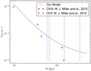 |
Fig. 1. Gas density model of the MilkyWay’s hot halo (black line) compared to observational data from Miller & Bregman (2015). The two vertical lines correspond to the minimal pericentre and maximal apocentre of the satellite orbits explored in this work (blue static potential and green evolving potential). |
3.1.2. Time evolution of the models
All along a Hubble time, a Milky Way-like galaxy see its mass growing through a succession of merger and accretion events. This mass grows and subsequently the increase of its gas halo and in particular its temperature through thermalisation has potentially a strong impact on the ram pressure and tidal stripping of its dwarf satellites. For this purpose, we considered the mass evolution of the MW model by defining three different evolution modes (EM). In all of them, the MW ends up with the same properties at z = 0:
-
Static (EM-{}): The MW does not evolve: Its potential remains fixed, equal to the one defined at z = 0. Similarly, the density and temperature of the halo gas stay constant.
-
Dynamic with a constant temperature (EM-{ρ}): The MW potential evolves through an increase of its total mass and size, together with the density of the hot component. The temperature of the gas is however kept fixed.
-
Dynamic with a dynamic temperature (EM-{ρ, T}): In addition to the second mode the gas temperature evolves too.
3.1.3. Mass and size evolution
Figure 2 displays the time evolution of the mass and size of our MW model used in the evolution mode EM-{ρ} and EM-{ρ, T}. Those curves are computed from the model Louise of the ELVIS simulations (Garrison-Kimmel et al. 2014), where the mass growth of several simulated galaxies is studied. The mass and size of the Louise galaxy is scaled in order to match exactly our non-evolving Milky Way model at z = 0. As in Garrison-Kimmel et al. (2014) the Louise galaxy was fitted using an NFW profile, we use the scale radius (Rs = Rvir/c) as a scaling for the Plummer softening parameter a.
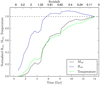 |
Fig. 2. Time evolution of the Milky Way parameters taken from the Louise galaxy (Mvir = 1012 M⊙ and Rvir = 261.3 kpc at z = 0) in the ELVIS (Garrison-Kimmel et al. 2014) simulations. The temperature is computed assuming a virial equilibrium at all time following Eq. (2). |
3.1.4. Temperature evolution
In the evolution mode EM-{ρ, T}, in addition to the density, we evolve the temperature T as show in Fig. 2. T is computed assuming a virial equilibrium of the halo gas at any time, using the following equation:
 (2)
(2)
where Mvir(t) and Rvir(t) are respectively the time-evolving virial mass and radius, mp the proton mass, G the gravitational constant, and kb is the Boltzmann constant. The Plummer softening parameter a is chosen in order to match the scale radius Rs = Rvir/c.
3.2. Satellite orbits
For the moving box simulations, we used only one generic orbit for the satellites galaxies. A deeper analysis of the influence of the orbital parameters on the dwarfs has been previously done with GEAR in Nichols et al. (2014).
According to recent proper motions and orbital parameters determination of dwarf galaxies based on the Gaia DR2 (Fritz et al. 2018), confirming earlier studies (Piatek et al. 2003, 2007), classical dwarfs such as Carina, Sextans and Sculptor have orbits with perigalacticon between 40 and 120 kpc and apogalacticon between 90 and 270 kpc (Fritz et al. 2018). It is worth noting that those measurements allow a fairly large interval of the orbital parameters. Therefore we decided to use a generic orbit with a pericentre of 60 kpc and an apocentre of 150 kpc, together with a current position of the dwarf at a distance of 85 kpc, with a negative velocity along the radial axis.
We emphasize here that wind tunnel simulations are very complementary to the moving box approach. Indeed they allow to explore a much larger parameter space of the hot gas temperature and density and infalling velocity of the satellites, than could be efficiently done with the moving boxes. In that respect, one does not need to sample a very large sets of orbits, as those would duplicate the parameters investigated by the wind tunnels.
We also recall that due to the constraints imposed by the moving box method (see Sect. 2.3), we are unable to use orbits with a pericentre smaller than 30 kpc, as the latter must be larger than half of our box size. To get the initial position of the extracted satellite at the infall time, z = zext, the orbit of a point mass is backward time-integrated in both the static (EM-{} mode) and evolving (EM-{ρ} and EM-{ρ, T} modes) MW potential, using a Runge-Kutta algorithm. The two orbits obtained are compared in Fig. 3. In the static case, the satellite will perform two and a half orbit around the MW, while only one and a half in the evolving case.
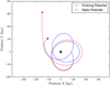 |
Fig. 3. Orbit used for the static (EM-{} mode) and evolving (EM-{ρ} and EM-{ρ, T} modes) MW potentials. The black diamond indicates the potential centre. The two points show the initial position at z = zext = 2.4. The final position is the same for both potentials and is situated at the coordinate [0, 85] kpc. |
4. Simulations
4.1. Wind tunnel simulations
Those simulations explore the effect of the wind parameters on the evolution of the dwarf. Precisely, we explored its velocity relative to the dwarf νw, its temperature Tw and density ρw. We preformed in total 96 simulations corresponding to each combination of the wind parameters as presented in Table 2. Each parameter is varied in a range of almost one dex around a fiducial value. They are set in order to match the observed MW constraints, either the gas density (Miller & Bregman 2013, 2015) or the satellites velocities constraints by their proper motions (Piatek et al. 2003, 2007).
Wind parameters used in the wind tunnel simulations.
The fiducial parameters of the wind are chosen to match our static Milky Way model at injection position. They are set to a density ρw = 1.66 × 10⁻⁵ atom cm−3, a velocity νw = 100 km s−1 and a temperature Tw = 2 × 10⁶ K). The bottom line of Table 2 indicates the ratio of the parameters with respect to the fiducial ones.
As presented in Sect. 3.1, we exposed the dwarf model h159 to the wind. This galaxy presents a rather shallow gravity potential, therefore the RP is efficient at stripping the gas and makes it sensitive to the wind parameters. Its initial cold (T ≤ 1000 K) and hot (T > 1000 K) gas mass at infall time, z = zext is respectively 4.58 and 27.0 × 10⁶ M⊙. 6 more massive galaxies have been also simulated (see Table A.1) confirming results obtained by model h159.
4.2. Moving box simulations
Those simulations explore the impact of the MW on the evolution of dwarf galaxies through a most complete interaction model which takes into account the orbits of the dwarf satellite through a time-variation of the wind parameters, but also the gravitational tidal effects together with the mass growth of the MW over a Hubble time.
We studied the evolution of 7 dwarfs, with total halo masses from M200 = 5.4 to 26.2 × 10⁸ M⊙. In the following, we will only focus on two representative models, the quenched model h159 dominated by old stellar populations and the Sculptor-like model h070 which has an extended star formation history. Other models, including more massive ones characterized by a sustained star formation rates give similar results. See Table A.2 for the list of additional models simulated. In a first step, each of these two dwarfs have been simulated in isolation. In a second step, they have been simulated in the three modes including the Milky Way interaction, EM-{}, EM-{ρ} and EM-{ρ, T}.
In Table 3, the parameters of each moving box and isolated fiducial simulations are given.
Description of the realistic simulations.
5. Results
5.1. Analysis
5.1.1. Pressure ratio
During the infall of a dwarf galaxy towards its host, the hot halo gas of the latter not only exerts a ram pressure against the ISM of the former, but also an almost uniform thermal pressure (TP) all around it. A key point to understand how the dwarf galaxy evolution is impacted upon infall, is to measure the individual effect of both the RP and TP, as they both have an opposite effect. While the RP removes the gas from the galaxy by momentum transfer, the TP tends to protect it by applying an additional force all around it, which prevents its removal due to RP, SNe feedback or UV-background heating resulting from the UV-photons emitted by active nuclei and star-forming galaxies. As presented by Sarazin (1986), the ram pressure is given by

where ρw is the wind density and νw its velocity. The thermal pressure is given by the ideal gas law

where n is the particle number density, kB the Boltzmann constant and Tw the wind temperature. Consequently, ratio of TP and RP which defines a unitless coefficient is written as
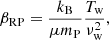 (3)
(3)
where μ the mean molecular mass and mP the proton mass.
We will see that this ratio will play a crucial role in the analysis and understanding of our simulations. It is worth noting that in Eq. (3), the density disappears and therefore the RP striping is independent of it at first order.
5.1.2. Gas fraction computation
In order to estimate the effect of RP stripping, we compute the gas fraction of our dwarf galaxies with time. It is performed by computing the mass of the hot gas in a constant radius taken as the initial virial radius R200(zinit). As contrary to the hot gas, the cold gas is concentrated around the dwarf centre, we computed the cold gas mass in a radius Rcg equal to 10% of R200(zinit).
5.2. Wind tunnel simulations
Our wind tunnel simulations confirm the strong effect the hot halo gas has on the dwarf ISM through RP. However they also reveal the importance of the satellite’s ISM multiphase structure. In a first step, we therefore split our analysis according to the gas temperature. In a second step, we will explore the effect on the star formation and study the impact of the wind parameters. A short summary will be given at the end of the section.
5.2.1. Stripping of the hot gas
Figure 4 shows the evolution of model h159 exposed to a wind of temperature equal to 3.39 × 10⁶ K, a density of 1.28 × 10⁻⁵ atom cm−3 and a velocity of 76.9 km s−1. This time sequence shows four different important steps. The first frame shows the gas at t = 2.1 Gyr, before any hydrodynamic interaction between the wind and the dwarf. The second one shows the first contact, the third one shows the state of the dwarf about one Gyr after the first contact. The last one corresponds to the steady state reached after the RP stripping. As expected, soon after the first contact, the large hot halo gas of the dwarf is strongly distorted (t = 2.6 Gyr) and quickly stripped, forming a trailing tail beyond the dwarf (t = 3.4 Gyr). At later time, only a small hot halo gas remains around the dwarf. The latter was not initially part of the dwarf halo gas. It results from the permanent heating of the cold gas by both UV-background heating and supernovae feedback. The efficient stripping of the hot gas is confirmed by the left panel of Fig. 5 where the time evolution of the hot gas fraction is shown for all of our 96 wind tunnel simulations. The colour of each line corresponds to the parameter βRP, the ratio between the thermal and ram pressure (Eq. (3)). All simulations show a quick drop of their hot gas fraction, indicating the efficient stripping of the dwarf hot halo. This demonstrates that the ram pressure stripping is captured in our simulations. The left panel of Fig. 5 also reveals a weak dependency on βRP. Winds characterized by a smaller βRP are more efficient to ram pressure strip the hot dwarf gas. Finally, we see that the isolated case traced by the green curve retains more hot gas after 4 Gyr as the latter do not suffer any ram pressure stripping. However, at later time the warm gas fraction decreases. This reveals the secular evaporation of the hot gas due to the continuous UV-background heating, until complete evaporation at t ≅ 9 Gyr. The remaining of hot gas in the wind tunnel simulations after that time compared to the isolated model will be discussed below.
 |
Fig. 4. Evolution of the cold, hot and wind gas during the first contact between the dwarf galaxy and the hot halo in a wind tunnel simulation with a wind temperature of 3.39 K, a density of 1.28 × 10⁻⁵ atom cm−3 and a velocity of 76.9 km s−1. The hot gas of the dwarf (Tw > 103 K) is shown in red, its cold gas (Tw < 103 K) in blue. The green colours trace the gas of the wind. This sequence shows how the hot dwarf gas is quickly stripped while its cold gas remains. |
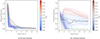 |
Fig. 5. Time evolution of the gas fraction of the dwarf galaxy h159 evolving through a wind tunnel simulation (see Table 2 for the list of parameters). Left panel: hot gas fraction contained in one virial radius. Right panel: cold gas fraction contained in 0.1 virial radius. The colour of each line reflect the corresponding βt. In both panels, the green and black lines correspond to the isolated and fiducial wind tunnel model respectively. A moving average has been applied with a gaussian kernel (standard deviation of ∼100 Myr in a window of −500 to 500 Myr) to reduce the noise. Due to this filter, the earliest times are removed and the different curves start at different fraction. |
5.2.2. Stripping of the cold gas
Contrary to the hot dwarf gas, the cold one is much more difficult to strip. This is well observed on the last panel of Fig. 4 at t = 5.1 Gyr, where even 3 Gyr after the first contact, cold gas is still present in the dwarf. The right panel of Fig. 5 shows in more detail, the time-evolution of the cold gas fraction for all our wind tunnel simulations. We split our models in two categories according to their βRP value: (i) thermal pressure-dominated models: βRP ≥ βt, red colours, (ii) ram pressure-dominated models: βRP < βt, blue colours, where βt is defined as the value at the transition and is about 3 for this galaxy.
Understanding the evolution in these different regimes first requires comprehension of the cold gas evolution in the isolated case. On the right panel of Fig. 5 the corresponding cold gas fraction is traced by the green curve. It is striking to see that the latter is dropping quickly, in less than 4 Gyr, faster than any other wind tunnel model. As for the hot gas, the origin of this drop is due to the UV-background ionizing photons which heat the gas. The potential well of this dwarf model being shallow, the latter evaporates (Efstathiou 1992; Quinn et al. 1996; Bullock et al. 2000; Noh & McQuinn 2014) resulting in the star formation quenching of the galaxy (Revaz & Jablonka 2018).
Thermal pressure-dominated models (βRP > βt). When the thermal pressure dominates over the ram pressure, the high pressurized wind compress the cold gas, protect it against ram pressure and act against its UV-background heating driven evaporation observed in the isolated case. This protection leads to keep up to 50% of cold gas, even after a Hubble time. The regular decrease of the mass fraction observed in this regime results from the conversion of the cold gas in to stars resulting from a continuous star formation rate. This point will be discussed further below.
Low wind velocity models show an important drop of the cold gas fraction followed by a strong rise between 2 and 4 Gyr. The drop results from some gas particles being pushed by the wind, leaving the cut off radius, where the cold gas is measured. However, those particles do not acquire enough kinetic energy to leave the galaxy and are thus slowly re-accreted by gravity, explaining the subsequent increase of the mass fraction.
The oscillations observed in nearly all models result from the continuously pulsation of the ISM induced by the numerous supernovae explosion which cause the gas to be ejected outwards Rcg (the radius used to compute the cold gas) before being slowly re-accreated.
Ram pressure-dominated models (βRP < βt). When the ram pressure dominates over the thermal pressure, the pressure protection is much weaker and the cold gas evolution becomes similar to the one of the isolated case. While just below the transition βt, cold gas may still survive up to z = 0, for very low βRP, it is lost. Those cases correspond to a fast moving dwarf with a speed larger than 150 km s−1 entering the halo of its host with a temperature of at most 1.3 × 10⁶ K. However, in any case when the ram pressure is present, the cold gas fraction remains larger than the isolated case. This indicates that the UV-background heating always dominates over the RP. The final loss is due to a supernovae that ejects almost all the gas further than the stripping radius which is then removed from the galaxy as a single cloud.
5.2.3. Impact on star formation
Together with an important change of the cold gas mass fraction with respect to the isolated model, our wind tunnel simulations strongly impact the star formation rate and subsequently the amount of stars formed. Figure 6 displays the cumulative number of stars formed with time. Compared to the star formation history, this plot has the advantage of being much less noisy.
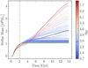 |
Fig. 6. Stellar mass as a function of time for the wind tunnel simulations. The colour is defined by the coefficient βRP in Eq. (3). The black line corresponds to our fiducial wind parameters. The green line corresponds to the isolated case. The blue dashed line represents the injection time. |
All wind tunnel models form stars more efficiently compared to the isolated case as a consequence of the remaining large reservoir of cold gas. For the extreme thermal pressure-dominated models, the final stellar mass is up to four times larger than the isolated galaxy model while the ram pressure-dominated models with very low βRP remains similar. It is worth nothing that pressure-dominated models with very low βRP, the ones that lost all their cold gas before z = 0, still display truncated star formation histories, however, much more extended than the isolated case, up to 9 Gyr in the most extreme case
For the sake of clarity, we note a small difference between all models, in the amount of stars formed before the injection time at z = zext, indicated by a vertical dashed line. Indeed, in order to computed the evolution of the stellar mass, we extracted all stellar particles in the dwarf at z = 0 and used their age to deduce the stellar mass present at any cosmic time. Consequently, star particles formed in the dwarf but leaving the galaxy at later time are no longer uncounted for, which may induce a small bias and the scatter observed between the different models. This approach, contrary to others where the stellar mass is computed at any time during the evolution, is much more representative to what an observer would have obtained relying on stellar ages deduced from a colour-magnitude diagram at present time.
5.2.4. Effect of the wind parameters
Figure 7 shows the final cold gas fraction of our 96 wind tunnel simulations, as a function of the wind parameters, more precisely, its velocity (νw), density (ρw) and temperature (Tw). According to Eq. (3), for a fixed temperature, the parameter βRP only depends on νw, to the inverse of its square. We thus supplement the velocity-axis (y-axis) with its corresponding βRP-value on the right of each plot.
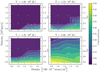 |
Fig. 7. Each plot represents the cold gas fraction at z = 0 of h159 as a function of the hot halo density and satellite velocity for different halo temperatures. The white circles are the simulations done. βRP is given on the right axis of each graph. Usually, the RPS is described only through density and velocity, but here the temperature dependency is shown to have an important impact. |
As expected in the theoretical formulas, νw and Tw are the two most sensitive parameters. For any temperature bin, increasing νw from 80 to 160 km s−1 move from a regime where the gas is protected, ending with an important cold gas mass fraction (between 0.3 and 0.5%) to a regime where all the gas is evaporated and the galaxy is quenched. Similarly, increasing Tw increases the thermal pressure which protect the dwarf gas. In strongly thermal pressure-dominated regimes (βRP > βt), a dwarf galaxy is thus able to protect its gas reservoir from stripping, up to 50%. On the contrary, from Eq. (3), the wind density has a limited impact on the galaxy gas fraction. However, it has a threshold effect. Indeed, for temperature between 1.3 and 1.76 × 10⁶ K, below a density of about 1.2 to 1.4 × 10⁻⁵ atom cm−3, the ram pressure stripping is enhanced, for a fixed νw and Tw. Extrapolating Fig. 7 to lower temperature, we can predict that a quenched dwarf, like our h159 model, orbiting in a halo with a temperature Tw < 1.3 × 10⁶ K and a density ρw < 2 × 10⁻⁵ atom cm−3 will loose all its gas.
5.3. Moving box simulations
In this section, we go one step further by supplementing our wind tunnel simulations with tidal stripping induced by a realistic Milky Way model environment. We also study the time-variation of the wind parameters all along the dwarf orbit which reflects the inhomogeneous hot halo of the Milky Way but also its growth with time. A summary of the final properties of the six simulations performed are given in Table 4.
Properties at z = 0 of the dwarf models evolved in the moving box simulations.
5.3.1. Effect of the Milky Way model
Figure 8 displays the star formation rate and time evolution of the cumulative stellar mass for each of the four cases studied for the two dwarf models h159 and h070, namely, isolated, EM-{}, EM-{ρ} and EM-{ρ, T}. For the three last cases that include the ram pressure stripping, the bottom panel of Fig. 9 shows the corresponding evolution of the coefficient βRP, while the top panel shows the distance of the dwarf with respect to its host galaxy (top panel).
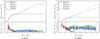 |
Fig. 8. Time evolution of the cumulative stellar mass (top) and star formation rate (bottom) of model h159 (left) and h070 (right), in the four models: isolated (black), EM-{} (blue), EM-{ρ} (green) and EM-{ρ, T} (red). The vertical dashed line indicates the injection time for models EM-{}, EM-{ρ} and EM-{ρ, T}. |
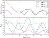 |
Fig. 9. Top panel: time evolution of the distance of the dwarfs for both the models h159 and h070 with respect to their host galaxy centre. Bottom panel: corresponding evolution of the βRP parameter all along the dwarf orbit. The blue, green and red curves correspond respectively to the EM-{}, EM-{ρ} and EM-{ρ, T}. The black line represents our fiducial wind tunnel simulation (black line in Figure 5). |
As discussed in Revaz & Jablonka (2018), when evolved in isolation, both models exhibit a star formation quenched after respectively ∼3 and ∼6 Gyr (black curves). However, when the dwarfs enter a static Milky Way halo (EM-{}, blue curve) at z = zext, the star formation is no longer quenched but becomes continuous. As a consequence, the resulting final stellar mass is up to four times the one of the isolated case. This increase of the star formation is due to the high βRP which pressurize the gas of the dwarf. As seen in Fig. 9, βRP oscillates between 3 and 0.5 reflecting the dwarf orbit. Maximal values of 3, similar to our fiducial wind tunnel simulation, are reached during the apocentre passage, when the dwarf has the lowest velocity. On the contrary, at the pericentre passage, at a distance of 50 kpc, higher velocities increase the ram pressure with respect to the thermal one and βRP drop down to 0.5. It is important to notice that even after four passages at the pericentre, the tidal force has not being strong enough to destroy the dwarf. This point is illustrated by the dark matter and stellar density profiles further discussed in Fig. 10.
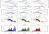 |
Fig. 10. Properties of the different simulations in a moving box. From left to right, the simulations are h159_sta, h159_dyn and h159_tem and in black h159_iso. In the first line, the density profile is shown for the total mass (straight lines) and the stellar mass (dashed lines). In the second line, the circular velocity and line of sight velocity dispersion are shown. In the third line, the stellar [Mg/Fe] vs. [Fe/H] distribution is shown. The orange crosses (pentagons) are observations of the LMC bar (inner disc) (Van der Swaelmen et al. 2013). In the last line, the metallicity distribution is shown. |
The green curve (EM-{ρ}) corresponds to the case where the Milky Way increases its mass and density but keep a constant hot gas temperature. The Milky Way mass growth directly impacts on the dwarf orbit which experiments only three passages at the pericentre. It also impact on the βRP parameter which starts with slightly higher values reflecting an initial larger distance (∼350 kpc) and lower orbital velocity. As the density is initially much lower, a factor of about 30 compared to EM-{}, the dwarf cold gas is slightly less confined by the hot Milky Way halo (density threshold effect as shown in Fig. 7) and can evaporates. For model h159, this leads to the decrease of the averaged star formation rate with respect to the static model (EM-{}). This effect is however not seen in model h070 for which the star formation rate of the EM-{ρ} model exceeds the one with model EM-{}. While a deeper analysis would be needed here, we interpret this difference by the deeper potential well of model h070 compared to model h159 at z = zext. In this case, the gravitational confinement of the gas dominates over the pressure one. Finally, when the hot gas temperature scales with respect to the gas density (EM-{ρ, T}, red curves), at the infall time, the thermal pressure of the hot gas is no longer present to confine the dwarf gas, as shown by its very low βRP in Fig. 9. Despite its increase at later time (t > 6 Gyr), the ram pressure stripping no longer impact the dwarf, as its cold gas already evaporated. In this model, both dwarf exhibit a star formation rate comparable to the isolated case sharing the same final stellar mass. As discussed in Sect. 5.2.3, the small differences at time t < 2 Gyr is due to the method used to compute the stellar content of the dwarf.
5.3.2. Impact on the final dwarf properties
Figures 10 and 11 present the final properties of the three interacting models of the dwarf h159 and h070 with the Milky Way, compared to their reference model in isolation.
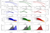 |
Fig. 11. Properties of the different simulations in a moving box. From left to right, the simulations correspond to h070_sta (blue), h070_dyn (green) and h070_tem (red) and are compared to the isolated model h070_iso in grey. In the first line, the density profile is shown for the total mass (straight lines) and the stellar mass (dashed lines). In the second line, the circular velocity and line of sight velocity dispersion are shown. In the third line, the stellar [Mg/Fe] vs. [Fe/H] distribution is shown. The orange crosses (pentagons) are observations of the LMC bar (inner disc) (Van der Swaelmen et al. 2013). In the last line, the metallicity distribution is shown. |
In those two figures, the first row displays the stellar density profile (dashed line) along with the total density profile including the dark halo (continuous line). While none of the interacting models are destroyed, they all show clear sign of stripping at radius larger than about 1 kpc, where the total density profiles drop compared to the isolated case. With four passages at the pericentre, h159_sta and h070_sta (EM-{}) are the most affected ones. They also see their total density profiles reduced up to 30% in the inner regions. However, due to their extended star formation rates, both models _sta and _rho exhibit a denser stellar density profile. On the contrary, with its quenched star formation history, the stellar profile of h159_tem is similar to the isolated case.
The tidal stripping also impacts the stellar line of sight velocity dispersion profile showed in the second row. In five of the six interacting models, the velocity dispersion is lower than in the isolated case, up to 5 km s−1 for the h159_sta model. This decrease reflects the adiabatic decompression after the removal of the outer dark halo, also responsible of the reduction of the circular velocity. It is worth noting that this stripping could help reproduce the low velocity dispersion (down to 5 km s−1) observed in six Andromeda galaxies and difficult to reproduce in isolated models (Revaz & Jablonka 2018). Only model h070_dyn sees its velocity dispersion and circular velocity increase in the central regions. This reflects its larger stellar content owing to its higher star formation rate.
The third and fourth rows of Figs. 10 and 11 compare the final chemical properties of the simulated dwarfs. The third row displays the abundance ratio of α-elements, traced here by the magnesium as a function of [Fe/H]. Because the dwarf galaxies enter their host halo at t ≅ 2 Gyr, the old metal poor stellar population ([Fe/H] ≲ −1.5) is not affected by the interaction. The stellar [Mg/Fe] vs. [Fe/H] distribution is characterized by a plateau at very low metallicity ([Fe/H] ≲ −2.5) followed by a decrease of [Mg/Fe], corresponding to the period where SNeIa yields dominates overs the SNeII, due to the drop of the star formation rate. In both the _sta and _rho models, the interaction with the hot gas halo leads to the extension of the star formation period. Therefore a new set of SNeII explode at a continuous rate and produce a constant injection of α-elements, quickly locked into new formed stars. This results into the formation of a plateau in [Mg/Fe] extending from [Fe/H] ≅ −1.5 to [Fe/H] ≅ −0.5 for model h159 and [Fe/H] ≅ −1.4 to [Fe/H] ≅ −0.2 for model h070. The large amount of stars formed at those metallicities are responsible of a peak in the metallicity distribution function shown in the fourth row. This peak is strongly shifted towards higher metallicities compared to the isolated case. While [Mg/Fe] plateau have been observed for metal rich ([Fe/H] ⪆ − 0.6) stellar population in Sagitarius (Hasselquist et al. 2017; Carlin et al. 2018), Fornax and LMC (Van der Swaelmen et al. 2013), and at a lower lever for Sculptor (see Fig. 11 of Tolstoy et al. 2009), they are found at solar or sub-solar [Mg/Fe], much lower than the one obtained here. A similar plateau may be obtained, to a somewhat shorter extension, for the brightest dwarf models of Revaz & Jablonka (2018). While a dedicated study will be necessary, we claim that such plateau could also be obtained if h070 would have entered its host halo at about 4–5 Gyr, the time needed to decrease [Mg/Fe] down to solar values, as shown in Fig. 11.
Finally, as their star formation history are similar to the isolated case, model h159_tem and h070_tem (EM-{ρ, T}) do not display any significant difference in their final chemical properties.
6. Discussion
Contrary to the widespread idea that local group dwarf spheroidal galaxies are easily quenched and devoid of gas due to the ram pressure stripping induced by its hot host halo, our simulations reveal a more complex picture. Both our wind tunnel and moving box simulations show that, while the hot gas of the dwarf is quickly ram pressure stripped, its cold and clumpy gas is not. On the contrary, due to the confinement of this gas by the thermal pressure of the hot halo gas which hamper the evaporation of the dwarf gas, the mass fraction of this cold phase can stay much above the one observed in the isolated case. Consequently depending on the orbital parameters of the dwarf, its infall time and the temperature of the host galaxy hot halo, the star formation of the dwarf may be extended over several Gyr or even heavily sustained up to the present time.
6.1. Comparison with other simulations
Numerous publications have been dedicated to the study of ram pressure stripping of galaxies, including our own.
Some of them concluded to the efficient stripping of gas implying the truncation or dampening of star formation (Mayer et al. 2006; Yozin & Bekki 2015; Fillingham et al. 2016; Emerick et al. 2016; Steinhauser et al. 2016). On the contrary, others concluded to the enhancement or reignition of the star formation (Bekki & Couch 2003; Kronberger et al. 2008; Kapferer et al. 2009; Nichols et al. 2015; Salem et al. 2015; Henderson & Bekki 2016; Wright et al. 2019). While a bunch of studies concluded that ram pressure may lead to both effects (Bahe et al. 2012; Bekki 2014) or no major effect (Williamson & Martel 2018). Those differences suggest that conclusions reached could strongly depend on the numerical methods used as well as the way the baryonic physics is implemented. Indeed, in those studies, a variety of hydrodynamical methods have been used. Those simulations relie on lagrangian SPH methods, with or without modern pressure-entropy formulation, eulerian methods with or without adaptive mesh refinement, or hybrid ones like moving-mesh methods. They differ by specific implementations of the ISM treatment, like radiative gas cooling below 104 K, external UV-background heating, hydrogen self-shielding against the UV-ionizing photons or magnetic field. Finally, they covers a large resolution range.
We discuss hereafter differences in our approach compared to other works that may lead to discrepancies, but also review works in different contexts that support our conclusions. Finally, will discuss our results in an observational context.
6.1.1. Stripping in dwarf galaxies
In a seminal paper, Mayer et al. (2006) showed that ram pressure stripping was efficient at completely removing the dwarf satellite ISM as long as they have a sufficiently low pericentre. However in their approach, the gas is not allowed to radiatively cool below 104 K. Under those conditions, the gas stays in a warm-hot and diffuse phase which is indeed easy to strip, as we demonstrated in Sect. 5.2.1. When the gas is allowed to cool down to lower temperature, it becomes clumpy (see Fig. 4 of Revaz & Jablonka 2018) and exposes a smaller surface to the wind hampering an efficient momentum transfer between the wind and the cold gas. Efficient satellite ram pressure stripping have also been recently mentioned by Simpson et al. (2018), where the quenching of satellite star formation in 30 cosmological zoom simulations of Milky Way-like galaxies have been studied. In these simulations, up to 90% of satellites with stellar mass equal to about 106 M⊙ are quenched, with ram pressure stripping being identified to be the dominant acting mechanism. This is nicely illustrated in their Fig. 8. However, those simulations also reveal a lack of any cold and clumpy phase which would be difficult to strip. In addition to a slightly lower resolution compared to ours, the absence of cold phase is the result of the stiff equation of state used, that represents a two-phase medium in pressure equilibrium (Springel & Hernquist 2003). However, it prevents the gas to cool down to low temperatures.
Recently, in high resolution simulation, Emerick et al. (2016) studied the ram pressure stripping of Leo T-like galaxies, including the effect of supernovae, and the presence of cold gas gas. However, they do not include a fully self-consistent star formation method, supernova being exploded at a location determined by a randomly sampled exponentially decreasing probability distribution centred on the galaxy. While concluding that the RP is unable to completely quench these type of galaxies in less than 2 Gyr, they show a clear decrease of the cold gas, contradicting our results. While being cooler and denser that the gas considered in Mayer et al. (2006) due to a temperature floor of 6 × 10³ K, as illustrated by their Fig. 3, it is nevertheless not as clumpy as the one considered in our work.
6.1.2. Thermal pressure confinement
One of the key effect that prevent the cold gas to evaporate and help sustain the star formation in our simulations is the thermal pressure confinement of hot ambient gas. We show hereafter that this effect is not only specific to our simulations but has been observed in other contexts.
Relying on SPH N-body simulations, Bekki & Couch (2003) studied the hydrodynamical effects of the hot ICM on a self-gravitating molecular gas in a spiral galaxy. They concluded that the high pressure of the Intra Cluster Medium (ICM) can trigger the collapse of molecular clouds leading to a burst of star formation. Along the same line, Kronberger et al. (2008) mentioned that in their models, the star formation rate is significantly enhanced by the ram-pressure effect (up to a factor of 3) when a disk galaxy move through an idealized ICM. Similarly, ram pressure can favour H2 formation (Henderson & Bekki 2016), indirectly boosting the formation of stars.
Mulchaey & Jeltema (2010) observed the hot halo surrounding galaxies and found a deficit of X-ray in comparison to the K-band luminosity for field galaxies, when compared to the galaxies in groups or cluster. They interpreted this results as the possibility that, contrary to field galaxies than can loose gas by supernova-driven winds, galaxies in groups or clusters see this outflowing material being pressure confined, preventing it to leave the galaxy halo.
In a more quantitative way, using the GIMIC simulations, Bahe et al. (2012) explored the pressure confinement by studying its effect on normal galaxies falling in groups or cluster, directly computing the coefficient βRP. In their simulations, they found 16% of their galaxies to be dominated by thermal pressure.
Sign of star formation increase due to confinement pressure have been also mentioned for simulation at a dwarf scale. This effect has been described by Nichols et al. (2015) in their dwarf spheroidal simulations with however a star formation boost lower than the ones obtain in the present paper. While this study also relied on the moving box technique, the physical prescriptions used where not comparable to the one used in the present study. The simulations where run out of any cosmological context and neither UV-background nor hydrogen self-shielding where considered.
Williamson & Martel (2018) used a technique similar to our moving box and observed a thermal confinement. While the ram pressure has a negligible impact on the star formation, they showed that the outflows are confined and slightly increase the metallicity of the dwarf.
Wright et al. (2019) observed that in their cosmological simulations, dwarf galaxies can re-ignite star formation, following the complete quenching of the galaxy due to UV-background heating. This re-ignition results from the compression of remaining hot gas in the dwarf halo, following an interaction with streams of gas in the Inter Galactic Medium (IGM). Those gas streams being either due to cosmic filaments or resulting from nearby galaxy mergers. This mechanism is particularly efficient when the ram pressure is low compared to the thermal pressure (high βRP), which corroborates with our own results.
6.2. Comparison with observations
From the observational point of view, the idea that satellites galaxies have been ram pressured stripped is mainly supported by the morphology-density relation observed in the Local Group (Einasto et al. 1974; van den Bergh 1994; Grcevich & Putman 2010). Quenched gas-poor spheroidals galaxies are found in the vicinity of their host galaxy (R ≲ 300 kpc) while star forming gas-rich dwarf irregulars are found at larger distances. At the exception of Leo I, Fornax and Carina that show a very recent quenching time (see for example Skillman et al. 2017) the majority of dSphs have been quenched at least 5 Gyr ago.
We point out that recent observational facts suggest that the morphology-density relation may not be universal. Indeed, spectroscopic observations of satellites galaxies around the NGC 4258 group showed that the majority of the 16 detected probable and possible satellites, lying within a 250 kpc, with a V-band magnitude down to −12, appears to be blue star-forming irregular galaxies in the SDSS image (Spencer et al. 2014). This is in strong contrast with the observations of the Local Group.
More recently, the SAGA survey (Geha et al. 2017) observed satellites companions around eight Milky Ways analogues, with luminosities down to the one of Leo I (Mr < −12.3), equivalent to about M⋆ = 106 M⊙ for star forming galaxies and M⋆ = 107 M⊙ for quenched galaxies. They found that among the 27 dwarf detected, the majority, 26 galaxies are star forming. This results points towards a less efficient quenching in those galaxies, compared the Milky Way.
The star formation rate of our models is strongly dependent on the infall time of the satellite relatively to the time when the galaxy halo is sufficiently hot and dense. As shown in Sect. 5.3.1 when the secular increase of the density and its temperature are taken into account, the evolution of the dwarfs entering the halo before a redshift of 2.4 are hardly different from those of their isolated counterparts. In that case the thermal pressure is unable to confine the gas of the satellites. This possibly could reflect that the different satellite population observed between the Milky Way and M31 and the ones of the SAGA survey could simply reflect a difference in the assembly history of the host galaxies.
6.3. Additional potential heating/cooling sources
As mentioned in Sect. 2.1, our current cooling implementation does not include H2. Adding this efficient coolant will increase the fragmentation of the gas, making it even more clumpy, strengthening our results.
It is worth mentioning that increasing the heating of the dwarf ISM could obviously help in quenching the star formation by ejecting more gas. Boosting the stellar feedback is not a viable solution as it would fail to reproduce the chemical observed properties of dwarf galaxies (Revaz & Jablonka 2018).
Another possible heating source is the thermal conduction between the MW’s hot halo and the dwarf’s cold gas. Cowie & McKee (1977) and McKee & Cowie (1977) developed an analytical model for the evaporation of an isolated spherical cloud in a hot gas. They considered both classical (electrons’ mean free path smaller than the cloud size) and saturated thermal conduction (electrons’ mean free path comparable to the cloud). Their analytical model shows that our dwarfs do not enter any saturated regime and are only marginally dominated by radiation loss. While detailed numerical simulations would be necessary to provide a conclusive answer, this first approximation predicts an evaporation over several Gyr.
Finally, considering the high UV-flux emitted by the proto-host Galaxy (van den Bergh 1994) or the potential strong impact of an AGN could help in removing the remaining confined gas.
7. Conclusions
We have presented high resolution GEAR-simulations of the interaction of dwarf spheroidal galaxies formed in a cosmological ΛCDM context with a Milky Way-like galaxy. We first ran a large set of wind tunnel simulations focusing on the hydrodynamical interaction between the dwarf system and the MW hot halo gas. We varied the wind parameters, which describe the velocity at which the dwarf enters the hot halo and orbits around the central galaxy, as well as the density and the temperature of the host halo gas. This allowed us to investigate how the ISM of the dwarf satellite was modified and to infer how its cold and hot gas phases could be ram pressure stripped. In a second step, we performed a set of moving box simulations that added the gravitational tidal interactions to the hydrodynamical ones. We also included the variation of the density and temperature of the hot halo all along the dwarf orbit as well as their increase due to the secular growth of the Milky Way.
The conclusions we reach are significantly different from those of previous works. Indeed, it turns out that including the hydrogen-self shielding that allows the gas to cool much below 104 K, leading to a multiphase ISM, absent in most of the previous studies, is essential to capture the effect of the ram pressure stripping and its impact on the dwarf star formation history.
Our results can be summarized as follows:
-
While the hot and diffuse gas phase of the dwarf (T > 1000 K) is efficiently and quickly stripped by the ram pressure induced by the gas of its host halo, the cold, star forming and clumpy gas phase (T < 1000 K) is not necessarily. The efficiency of the stripping of this cold gas depends on the ratio between the thermal pressure and the ram pressure both exerted on the dwarf by the hot halo gas. When the thermal pressure is high, the cold gas is confined and its stripping is slowed down.
-
As a consequence of the above, the infall time of a dwarf galaxy plays a decisive role in the evolution of the dwarf satellites. If the interaction between the host galaxy and its satellite begins when the thermal pressure is low, that is the host halo is not sufficiently dense or hot, then, the evolution of the dwarf will be essentially the same as in isolation. The cold ISM will evaporate due to the UV-background heating and star formation will be quenched. On the contrary, the cold ISM is confined and remains attached to the dwarf.
-
The confinement of the cold gas in the dwarf satellite leads to an extension of its star formation history. While the same dwarf galaxy would see its star formation quenched due to the evaporation of the residual gas, its interaction with the Milky Way keeps the star formation rate roughly at the level it had when the dwarf entered the host halo. This translates into a higher final mean metallicity, by up to 1 dex in the examples presented in this study. Because our model dwarf spheroidals enter the Milky-Way like galaxy at ∼2 Gyr, their star formation rates have already significantly decreased, therefore the ejecta of the SNeIa explosion contribute significantly to the dwarf’s ISM enrichment. Hence, both our details models display an extended low, although still super-solar, [α/Fe] tail. A solar or sub-solar plateau similar to the Fornax or Sagittarius dwarf galaxy could be obtained if the dwarf enters the hot halo of its host galaxy at later time, where the [α/Fe] decreased to lower values. Firm conclusion on this point would require a dedicated and thorough investigation.
Ram-pressure and tidal interactions do not seem sufficient to explain by themselves the morphology-density relation observed in the Local Group. It would require very specific conditions, either a very late entry of the closest dSphs in the halo of the Milky Way, or a very early accretion before the end of the Galaxy mass assembly. Other processes might play a role, such as the heating by the UV-flux of the Milky Way itself.
Star forming satellites have been found around other Milky Way analogues or in groups (Spencer et al. 2014; Geha et al. 2017). As the effect on the hot host halo strongly depends on the infall time of the satellite galaxy, the different satellite populations observed between the Milky Way and M31 (dominance of quenched gas-poor galaxies) and the ones of the SAGA survey (star forming galaxies) could potentially reflect a difference in the assembly history of the host galaxies.
Acknowledgments
We are indebted to the International Space Science Institute (ISSI), Bern, Switzerland, for supporting and funding the international team “First stars in dwarf galaxies”. We are grateful to Matthew Nichols to help us with the moving box technique. We enjoyed discussions with Matthieu Schaller, Romain Teyssier, Françoise Combes, Allessandro Lupi, Andrew Emerick. This work was supported by the Swiss Federal Institute of Technology in Lausanne (EPFL) through the use of the facilities of its Scientific IT and Application Support Center (SCITAS). The simulations presented here were run on the Deneb clusters. The data reduction and galaxy maps have been performed using the parallelized Python pNbody package (http://lastro.epfl.ch/projects/pNbody/). We are grateful to the Numpy (Oliphant 2015), Matplotlib (Caswell et al. 2018) SciPy (Jones et al. 2001) and IPython (Perez & Granger 2007) teams for providing the scientific community with essential python tools.
References
- Arraki, K. S., Klypin, A., More, S., & Trujillo-Gomez, S. 2014, MNRAS, 438, 1466 [NASA ADS] [CrossRef] [Google Scholar]
- Atek, H., Richard, J., Jauzac, M., et al. 2015, ApJ, 814, 69 [NASA ADS] [CrossRef] [Google Scholar]
- Aubert, D., & Teyssier, R. 2010, ApJ, 724, 244 [NASA ADS] [CrossRef] [Google Scholar]
- Bahe, Y. M., McCarthy, I. G., Crain, R. A., & Theuns, T. 2012, MNRAS, 424, 1179 [NASA ADS] [CrossRef] [Google Scholar]
- Bekki, K. 2014, MNRAS, 438, 444 [NASA ADS] [CrossRef] [Google Scholar]
- Bekki, K., & Couch, W. J. 2003, ApJ, 596, L13 [NASA ADS] [CrossRef] [Google Scholar]
- Bouwens, R. J., Illingworth, G. D., Oesch, P. A., et al. 2015, ApJ, 803, 34 [NASA ADS] [CrossRef] [Google Scholar]
- Boylan-Kolchin, M., Bullock, J. S., & Kaplinghat, M. 2011, MNRAS, 415, L40 [CrossRef] [Google Scholar]
- Boylan-Kolchin, M., Bullock, J. S., & Kaplinghat, M. 2012, MNRAS, 422, 1203 [NASA ADS] [CrossRef] [Google Scholar]
- Bullock, J. S., & Boylan-Kolchin, M. 2017, ARA&A, 55, 343 [NASA ADS] [CrossRef] [Google Scholar]
- Bullock, J. S., Kravtsov, A. V., & Weinberg, D. H. 2000, ApJ, 539, 517 [NASA ADS] [CrossRef] [Google Scholar]
- Carlin, J. L., Sheffield, A. A., Cunha, K., & Smith, V. V. 2018, ApJ, 859, L10 [NASA ADS] [CrossRef] [Google Scholar]
- Caswell, T. A., Droettboom, M., & Hunter, J. 2018, matplotlib/matplotlib v3.0.2 [Google Scholar]
- Cloet-Osselaer, A., De Rijcke, S., Schroyen, J., & Dury, V. 2012, MNRAS, 423, 735 [NASA ADS] [CrossRef] [Google Scholar]
- Cloet-Osselaer, A., De Rijcke, S., Vandenbroucke, B., et al. 2014, MNRAS, 442, 2909 [NASA ADS] [CrossRef] [Google Scholar]
- Cowie, L. L., & McKee, C. F. 1977, ApJ, 211, 135 [NASA ADS] [CrossRef] [Google Scholar]
- de Boer, T. J. L., Tolstoy, E., & Hill, V. 2012, A&A, 544, A73 [NASA ADS] [CrossRef] [EDP Sciences] [Google Scholar]
- de Boer, T. J. L., Tolstoy, E., Lemasle, B., et al. 2014, A&A, 572, A10 [NASA ADS] [CrossRef] [EDP Sciences] [Google Scholar]
- Del Popolo, A., & Le Delliou, M. 2017, Galaxies, 5, 17 [NASA ADS] [CrossRef] [Google Scholar]
- Durier, F., & Vecchia, C. D. 2012, MNRAS, 419, 465 [NASA ADS] [CrossRef] [Google Scholar]
- Efstathiou, G. 1992, MNRAS, 256, 43P [Google Scholar]
- Einasto, J., Saar, E., Kaasik, A., & Chernin, A. D. 1974, Nature, 252, 111 [NASA ADS] [CrossRef] [Google Scholar]
- Emerick, A., Mac Low, M.-M., Grcevich, J., & Gatto, A. 2016, ApJ, 826, 148 [NASA ADS] [CrossRef] [Google Scholar]
- Escala, I., Wetzel, A., Kirby, E. N., et al. 2018, MNRAS, 474, 2194 [NASA ADS] [CrossRef] [Google Scholar]
- Ferland, G. J., Chatzikos, M., Guzmán, F., et al. 2017, Rev. Mex. Astron. Astrofis., 53, 385 [NASA ADS] [Google Scholar]
- Fillingham, S. P., Cooper, M. C., Pace, A. B., et al. 2016, MNRAS, 463, 1916 [NASA ADS] [CrossRef] [Google Scholar]
- Fitts, A., Boylan-Kolchin, M., Elbert, O. D., et al. 2017, MNRAS, 471, 3547 [NASA ADS] [CrossRef] [Google Scholar]
- Fitts, A., Boylan-Kolchin, M., Bullock, J. S., et al. 2018, MNRAS, 479, 319 [NASA ADS] [CrossRef] [Google Scholar]
- Fritz, T. K., Battaglia, G., Pawlowski, M. S., et al. 2018, A&A, 619, A103 [NASA ADS] [CrossRef] [EDP Sciences] [Google Scholar]
- Garrison-Kimmel, S., Boylan-Kolchin, M., Bullock, J. S., & Lee, K. 2014, MNRAS, 438, 2578 [NASA ADS] [CrossRef] [Google Scholar]
- Garrison-Kimmel, S., Hopkins, P. F., Wetzel, A., et al. 2018, MNRAS, submitted [arXiv:1806.04143] [Google Scholar]
- Geha, M., Wechsler, R. H., Mao, Y.-Y., et al. 2017, ApJ, 847, 4 [NASA ADS] [CrossRef] [Google Scholar]
- Grcevich, J., & Putman, M. E. 2010, ApJ, 721, 922 [NASA ADS] [CrossRef] [Google Scholar]
- Haardt, F., & Madau, P. 2012, ApJ, 746, 125 [NASA ADS] [CrossRef] [Google Scholar]
- Hahn, O., & Abel, T. 2011, MNRAS, 415, 2101 [NASA ADS] [CrossRef] [Google Scholar]
- Hasselquist, S., Shetrone, M., Smith, V., et al. 2017, ApJ, 845, 162 [NASA ADS] [CrossRef] [Google Scholar]
- Henderson, B., & Bekki, K. 2016, ApJ, 822, L33 [NASA ADS] [CrossRef] [Google Scholar]
- Hopkins, P. F. 2013, MNRAS, 428, 2840 [NASA ADS] [CrossRef] [Google Scholar]
- Hopkins, P. F., Quataert, E., & Murray, N. 2011, MNRAS, 417, 950 [NASA ADS] [CrossRef] [Google Scholar]
- Jones, E., Oliphant, T., Peterson, P., et al. 2001, SciPy: Open Source Scientific Tools for Python [Google Scholar]
- Kafle, P. R., Sharma, S., Lewis, G. F., & Bland-Hawthorn, J. 2014, ApJ, 794, 59 [NASA ADS] [CrossRef] [Google Scholar]
- Kapferer, W., Sluka, C., Schindler, S., Ferrari, C., & Ziegler, B. 2009, A&A, 499, 87 [NASA ADS] [CrossRef] [EDP Sciences] [Google Scholar]
- Klypin, A., Kravtsov, A. V., Valenzuela, O., & Prada, F. 1999, ApJ, 522, 82 [Google Scholar]
- Kobayashi, C., Tsujimoto, T., & Nomoto, K. 2000, ApJ, 539, 26 [NASA ADS] [CrossRef] [Google Scholar]
- Kronberger, T., Kapferer, W., Ferrari, C., Unterguggenberger, S., & Schindler, S. 2008, A&A, 481, 337 [NASA ADS] [CrossRef] [EDP Sciences] [Google Scholar]
- Kroupa, P. 2001, MNRAS, 322, 231 [NASA ADS] [CrossRef] [Google Scholar]
- Macció, A. V., Frings, J., Buck, T., et al. 2017, MNRAS, 472, 2356 [NASA ADS] [CrossRef] [Google Scholar]
- Mayer, L., Mastropietro, C., Wadsley, J., Stadel, J., & Moore, B. 2006, MNRAS, 369, 1021 [NASA ADS] [CrossRef] [Google Scholar]
- McConnachie, A. W. 2012, AJ, 144, 4 [NASA ADS] [CrossRef] [Google Scholar]
- McKee, C. F., & Cowie, L. L. 1977, ApJ, 215, 213 [NASA ADS] [CrossRef] [Google Scholar]
- McQuinn, K. B. W., Skillman, E. D., Dolphin, A., et al. 2015, ApJ, 812, 158 [NASA ADS] [CrossRef] [Google Scholar]
- Miller, M. J., & Bregman, J. N. 2013, ApJ, 770, 118 [NASA ADS] [CrossRef] [Google Scholar]
- Miller, M. J., & Bregman, J. N. 2015, ApJ, 800, 14 [NASA ADS] [CrossRef] [Google Scholar]
- Moore, B. 1994, Nature, 370, 629 [NASA ADS] [CrossRef] [Google Scholar]
- Moore, B., Ghigna, S., Governato, F., et al. 1999, ApJ, 524, L19 [Google Scholar]
- Mulchaey, J. S., & Jeltema, T. E. 2010, ApJ, 715, L1 [NASA ADS] [CrossRef] [Google Scholar]
- Navarro, J. F., Frenk, C. S., & White, S. D. M. 1996, ApJ, 462, 563 [NASA ADS] [CrossRef] [Google Scholar]
- Navarro, J. F., Frenk, C. S., & White, S. D. M. 1997, ApJ, 490, 493 [NASA ADS] [CrossRef] [Google Scholar]
- Nichols, M., Revaz, Y., & Jablonka, P. 2014, A&A, 564, A112 [NASA ADS] [CrossRef] [EDP Sciences] [Google Scholar]
- Nichols, M., Revaz, Y., & Jablonka, P. 2015, A&A, 582, A23 [NASA ADS] [CrossRef] [EDP Sciences] [Google Scholar]
- Noh, Y., & McQuinn, M. 2014, MNRAS, 444, 503 [NASA ADS] [CrossRef] [Google Scholar]
- Okamoto, T., Eke, V. R., Frenk, C. S., & Jenkins, A. 2005, MNRAS, 363, 1299 [NASA ADS] [CrossRef] [Google Scholar]
- Oliphant, T. E. 2015, Guide to NumPy, 2nd edn. (USA: CreateSpace Independent Publishing Platform) [Google Scholar]
- Perez, F., & Granger, B. E. 2007, Comput. Sci. Eng., 9, 21 [Google Scholar]
- Piatek, S., Pryor, C., Olszewski, E. W., et al. 2003, ApJ, 126, 2346 [NASA ADS] [CrossRef] [Google Scholar]
- Piatek, S., Pryor, C., Bristow, P., et al. 2007, ApJ, 133, 818 [NASA ADS] [CrossRef] [Google Scholar]
- Planck Collaboration Int. XXIV. 2015, A&A, 580, A22 [NASA ADS] [CrossRef] [EDP Sciences] [Google Scholar]
- Quinn, T., Katz, N., & Efstathiou, G. 1996, MNRAS, 278, L49 [NASA ADS] [CrossRef] [Google Scholar]
- Revaz, Y., & Jablonka, P. 2012, A&A, 538, A82 [NASA ADS] [CrossRef] [EDP Sciences] [Google Scholar]
- Revaz, Y., & Jablonka, P. 2018, A&A, 616, A96 [NASA ADS] [CrossRef] [EDP Sciences] [Google Scholar]
- Revaz, Y., Jablonka, P., Sawala, T., et al. 2009, A&A, 501, 189 [NASA ADS] [CrossRef] [EDP Sciences] [Google Scholar]
- Revaz, Y., Arnaudon, A., Nichols, M., Bonvin, V., & Jablonka, P. 2016, A&A, 588, A21 [NASA ADS] [CrossRef] [EDP Sciences] [Google Scholar]
- Robertson, B. E., Ellis, R. S., Furlanetto, S. R., & Dunlop, J. S. 2015, ApJ, 802, L19 [NASA ADS] [CrossRef] [Google Scholar]
- Salem, M., Besla, G., Bryan, G., et al. 2015, ApJ, 815, 77 [NASA ADS] [CrossRef] [Google Scholar]
- Sarazin, C. L. 1986, Rev. Mod. Phys., 58, 1 [NASA ADS] [CrossRef] [Google Scholar]
- Sawala, T., Scannapieco, C., Maio, U., & White, S. 2010, MNRAS, 402, 1599 [NASA ADS] [CrossRef] [Google Scholar]
- Sawala, T., Scannapieco, C., & White, S. 2012, MNRAS, 420, 1714 [NASA ADS] [CrossRef] [Google Scholar]
- Sawala, T., Frenk, C. S., Fattahi, A., et al. 2016, MNRAS, 457, 1931 [NASA ADS] [CrossRef] [Google Scholar]
- Schroyen, J., de Rijcke, S., Valcke, S., Cloet-Osselaer, A., & Dejonghe, H. 2011, MNRAS, 416, 601 [NASA ADS] [Google Scholar]
- Simpson, C. M., Grand, R. J. J., Gómez, F. A., et al. 2018, MNRAS, 478, 548 [NASA ADS] [CrossRef] [Google Scholar]
- Skillman, E. D., Monelli, M., Weisz, D. R., et al. 2017, ApJ, 837, 102 [NASA ADS] [CrossRef] [Google Scholar]
- Smith, B. D., Bryan, G. L., Glover, S. C. O., et al. 2017, MNRAS, 466, 2217 [NASA ADS] [CrossRef] [Google Scholar]
- Spencer, M., Loebman, S., & Yoachim, P. 2014, ApJ, 788, 146 [NASA ADS] [CrossRef] [Google Scholar]
- Springel, V. 2005, MNRAS, 364, 1105 [NASA ADS] [CrossRef] [Google Scholar]
- Springel, V., & Hernquist, L. 2003, MNRAS, 339, 289 [Google Scholar]
- Steinhauser, D., Schindler, S., & Springel, V. 2016, A&A, 591, A51 [NASA ADS] [CrossRef] [EDP Sciences] [Google Scholar]
- Stinson, G., Seth, A., Katz, N., et al. 2006, MNRAS, 373, 1074 [NASA ADS] [CrossRef] [Google Scholar]
- Tolstoy, E., Hill, V., & Tosi, M. 2009, ARA&A, 47, 371 [NASA ADS] [CrossRef] [Google Scholar]
- Tornatore, L., Borgani, S., Dolag, K., & Matteucci, F. 2007, MNRAS, 382, 1050 [NASA ADS] [CrossRef] [Google Scholar]
- Tsujimoto, T., Nomoto, K., Yoshii, Y., et al. 1995, MNRAS, 277, 945 [NASA ADS] [CrossRef] [Google Scholar]
- Valcke, S., de Rijcke, S., & Dejonghe, H. 2008, MNRAS, 389, 1111 [NASA ADS] [CrossRef] [Google Scholar]
- van den Bergh, S. 1994, ApJ, 107, 1328 [NASA ADS] [CrossRef] [Google Scholar]
- Van der Swaelmen, M., Hill, V., Primas, F., & Cole, A. A. 2013, A&A, 560, A44 [NASA ADS] [CrossRef] [EDP Sciences] [Google Scholar]
- Vazdekis, A., Casuso, E., Peletier, R. F., & Beckman, J. E. 1996, ApJS, 106, 307 [NASA ADS] [CrossRef] [Google Scholar]
- Weisz, D. R., Zucker, D. B., Dolphin, A. E., et al. 2012, ApJ, 748, 88 [NASA ADS] [CrossRef] [Google Scholar]
- Wetzel, A. R., Deason, A. J., & Garrison-Kimmel, S. 2015, ApJ, 807, 49 [NASA ADS] [CrossRef] [Google Scholar]
- Wetzel, A. R., Hopkins, P. F., Kim, J.-H., et al. 2016, ApJ, 827, L23 [NASA ADS] [CrossRef] [Google Scholar]
- Wiersma, R. P. C., Schaye, J., Theuns, T., Vecchia, C. D., & Tornatore, L. 2009, MNRAS, 399, 574 [NASA ADS] [CrossRef] [Google Scholar]
- Williamson, D., & Martel, H. 2018, ApJ, 867, 72 [NASA ADS] [CrossRef] [Google Scholar]
- Wright, A. C., Brooks, A. M., Weisz, D. R., & Christensen, C. R. 2019, MNRAS, 482, 1176 [NASA ADS] [CrossRef] [Google Scholar]
- Xue, X. X., Rix, H. W., Zhao, G., et al. 2008, ApJ, 684, 1143 [NASA ADS] [CrossRef] [Google Scholar]
- Yozin, C., & Bekki, K. 2015, MNRAS, 453, 14 [NASA ADS] [CrossRef] [Google Scholar]
Appendix A: Additional wind tunnel and moving box simulations
Additional wind tunnel simulations performed.
Additional moving box simulations performed.
All Tables
All Figures
|
Fig. 1. Gas density model of the MilkyWay’s hot halo (black line) compared to observational data from Miller & Bregman (2015). The two vertical lines correspond to the minimal pericentre and maximal apocentre of the satellite orbits explored in this work (blue static potential and green evolving potential). |
| In the text | |
|
Fig. 2. Time evolution of the Milky Way parameters taken from the Louise galaxy (Mvir = 1012 M⊙ and Rvir = 261.3 kpc at z = 0) in the ELVIS (Garrison-Kimmel et al. 2014) simulations. The temperature is computed assuming a virial equilibrium at all time following Eq. (2). |
| In the text | |
|
Fig. 3. Orbit used for the static (EM-{} mode) and evolving (EM-{ρ} and EM-{ρ, T} modes) MW potentials. The black diamond indicates the potential centre. The two points show the initial position at z = zext = 2.4. The final position is the same for both potentials and is situated at the coordinate [0, 85] kpc. |
| In the text | |
|
Fig. 4. Evolution of the cold, hot and wind gas during the first contact between the dwarf galaxy and the hot halo in a wind tunnel simulation with a wind temperature of 3.39 K, a density of 1.28 × 10⁻⁵ atom cm−3 and a velocity of 76.9 km s−1. The hot gas of the dwarf (Tw > 103 K) is shown in red, its cold gas (Tw < 103 K) in blue. The green colours trace the gas of the wind. This sequence shows how the hot dwarf gas is quickly stripped while its cold gas remains. |
| In the text | |
|
Fig. 5. Time evolution of the gas fraction of the dwarf galaxy h159 evolving through a wind tunnel simulation (see Table 2 for the list of parameters). Left panel: hot gas fraction contained in one virial radius. Right panel: cold gas fraction contained in 0.1 virial radius. The colour of each line reflect the corresponding βt. In both panels, the green and black lines correspond to the isolated and fiducial wind tunnel model respectively. A moving average has been applied with a gaussian kernel (standard deviation of ∼100 Myr in a window of −500 to 500 Myr) to reduce the noise. Due to this filter, the earliest times are removed and the different curves start at different fraction. |
| In the text | |
|
Fig. 6. Stellar mass as a function of time for the wind tunnel simulations. The colour is defined by the coefficient βRP in Eq. (3). The black line corresponds to our fiducial wind parameters. The green line corresponds to the isolated case. The blue dashed line represents the injection time. |
| In the text | |
|
Fig. 7. Each plot represents the cold gas fraction at z = 0 of h159 as a function of the hot halo density and satellite velocity for different halo temperatures. The white circles are the simulations done. βRP is given on the right axis of each graph. Usually, the RPS is described only through density and velocity, but here the temperature dependency is shown to have an important impact. |
| In the text | |
|
Fig. 8. Time evolution of the cumulative stellar mass (top) and star formation rate (bottom) of model h159 (left) and h070 (right), in the four models: isolated (black), EM-{} (blue), EM-{ρ} (green) and EM-{ρ, T} (red). The vertical dashed line indicates the injection time for models EM-{}, EM-{ρ} and EM-{ρ, T}. |
| In the text | |
|
Fig. 9. Top panel: time evolution of the distance of the dwarfs for both the models h159 and h070 with respect to their host galaxy centre. Bottom panel: corresponding evolution of the βRP parameter all along the dwarf orbit. The blue, green and red curves correspond respectively to the EM-{}, EM-{ρ} and EM-{ρ, T}. The black line represents our fiducial wind tunnel simulation (black line in Figure 5). |
| In the text | |
|
Fig. 10. Properties of the different simulations in a moving box. From left to right, the simulations are h159_sta, h159_dyn and h159_tem and in black h159_iso. In the first line, the density profile is shown for the total mass (straight lines) and the stellar mass (dashed lines). In the second line, the circular velocity and line of sight velocity dispersion are shown. In the third line, the stellar [Mg/Fe] vs. [Fe/H] distribution is shown. The orange crosses (pentagons) are observations of the LMC bar (inner disc) (Van der Swaelmen et al. 2013). In the last line, the metallicity distribution is shown. |
| In the text | |
|
Fig. 11. Properties of the different simulations in a moving box. From left to right, the simulations correspond to h070_sta (blue), h070_dyn (green) and h070_tem (red) and are compared to the isolated model h070_iso in grey. In the first line, the density profile is shown for the total mass (straight lines) and the stellar mass (dashed lines). In the second line, the circular velocity and line of sight velocity dispersion are shown. In the third line, the stellar [Mg/Fe] vs. [Fe/H] distribution is shown. The orange crosses (pentagons) are observations of the LMC bar (inner disc) (Van der Swaelmen et al. 2013). In the last line, the metallicity distribution is shown. |
| In the text | |
Current usage metrics show cumulative count of Article Views (full-text article views including HTML views, PDF and ePub downloads, according to the available data) and Abstracts Views on Vision4Press platform.
Data correspond to usage on the plateform after 2015. The current usage metrics is available 48-96 hours after online publication and is updated daily on week days.
Initial download of the metrics may take a while.