| Issue |
A&A
Volume 624, April 2019
|
|
|---|---|---|
| Article Number | A67 | |
| Number of page(s) | 16 | |
| Section | Cosmology (including clusters of galaxies) | |
| DOI | https://doi.org/10.1051/0004-6361/201833758 | |
| Published online | 12 April 2019 | |
The CMB angular power spectrum via component separation: a study on Planck data
1
Institut d’Astrophysique de Paris, Sorbonne Université, CNRS (UMR7095), 98 bis Boulevard Arago, 75014 Paris, France
e-mail: This email address is being protected from spambots. You need JavaScript enabled to view it.
2
Sorbonne Universités, Institut Lagrange de Paris (ILP), 98 bis Boulevard Arago, 75014 Paris, France
3
University of Cincinnati, Cincinnati, OH 45221, USA
4
APC, Univ Paris Diderot, CNRS/IN2P3, CEA/Irfu, Obs de Paris, Sorbonne Paris Cité, France
Received:
2
July
2018
Accepted:
19
October
2018
Abstract
Aims. We investigate the extent to which foreground-cleaned cosmic microwave background (CMB) maps can be used to estimate cosmological parameters at small scales.
Methods. We use the SMICA method, a blind separation technique that works directly at the spectral level. In this work we focus on the small scales of the CMB angular power spectrum, which are chiefly affected by noise and extragalactic foregrounds, such as point sources. We adapt SMICA to use only cross-spectra between data maps, thus avoiding the noise bias. In this study, performed using both simulations and Planck 2015 data, we fit for extragalactic point sources by modelling them as shot noise of two independent populations.
Results. In simulations, we correctly recover the point-source emission law, and obtain a CMB angular power spectrum that has an average foreground residual of one fifth of the CMB power at ℓ ≥ 2200. With Planck data, the recovered point-source emission law corresponds to external estimates, with some offsets at the highest and lowest frequencies, possibly due to frequency decoherence of point sources. The CMB angular power spectrum residuals are consistent with what we find in simulations. The cosmological parameters obtained from the simulations and the data show offsets up to 1σ on average from their expected values. Biases on cosmological parameters in simulations represent the expected level of bias in Planck data.
Conclusions. The results on cosmological parameters depend on the detail of the foreground residual contamination in the spectrum, and therefore a tailored modelling of the likelihood foreground model is required.
Key words: cosmic background radiation / cosmological parameters / methods: data analysis / methods: statistical
© C. Umiltà et al. 2019
 Open Access article, published by EDP Sciences, under the terms of the Creative Commons Attribution License (http://creativecommons.org/licenses/by/4.0), which permits unrestricted use, distribution, and reproduction in any medium, provided the original work is properly cited.
1. Introduction
The cosmic microwave background (CMB) is an important probe for cosmology, and in recent years a considerable amount of effort has been dedicated to its extraction from available data. In particular, the CMB angular power spectrum can be used to constrain the cosmological parameters. The Planck mission provided the astronomical community with full-sky observations in nine frequency bands between 30 and 857 GHz. These data are critical for CMB science since they allow to characterise and separate the primordial CMB signal from the other galactic and extragalactic emissions or “foregrounds”.
Separating the CMB from the foregrounds is a highly non-trivial task, and a number of component separation methods have been conceived in the past years. The Commander method (Eriksen et al. 2004, 2008) performs a Bayesian exploration of a physical parametric model. The spectral estimation via expectation maximization (SEVEM) method (Fernández-Cobos et al. 2012) fits a number of templates obtained from the data themselves, while the correlated component analysis (CCA; Bedini et al. 2005; Bonaldi et al. 2006) technique exploits the foregrounds spatial correlations to recover their emission law.
Blind techniques, which are techniques that use no prior information on foreground emission, have been widely employed. The advantage of these is that they do not require any assumption on the foreground contamination. We note that this applies to SEVEM as well. Among blind methods, many exploit the internal linear combination (ILC) technique: the needlet ILC (NILC; Delabrouille et al. 2009; Basak & Delabrouille 2012, 2013), the generalized needlet ILC (GNILC; Remazeilles et al. 2011), and more recently the scale-discretised, directional wavelet ILC (SILC; Rogers et al. 2016) and the harmonic-space ILC (HILC; Sudevan et al. 2017). The local generalized morphological component analysis (L-GMCA; Bobin et al. 2008, 2013) method exploits the sparsity of the data in the wavelet domain.
Another popular technique for blind source separation is the independent component analysis (ICA), implemented by the Fast ICA (FastICA; Maino et al. 2002), which is based on the non-Gaussianity of the sources, and also by the Bayesian ICA (BICA; Vansyngel et al. 2016), which implements ICA in a Bayesian framework, and the spectral matching ICA (SMICA; Cardoso et al. 2008), which blindly recovers the sources’ spectra in the maximum likelihood sense. An effort to find new tools for component separation is on-going: for example the ABS blind method has recently been proposed (Zhang et al. 2016).
The Planck collaboration has selected four different methods to perform component separation and produce CMB maps. These are Commander, NILC, SEVEM, and SMICA (Planck Collaboration IX 2016). Nevertheless, the cosmological analysis of the CMB is sensitive to residual foreground contamination in the data. The angular power spectra derived from the four Planck CMB maps have a residual foreground content which prevents their use for cosmological purposes. In particular, the small-scale residuals of unresolved point sources in these maps is not well characterised (Planck Collaboration XI 2016). Among the four CMB maps released by the Planck collaboration, the SMICA map has the lowest extragalactic contribution at high-ℓ (Planck Collaboration IX 2016). More importantly, SMICA proceeds in two steps: a component separation at the spectral (harmonic) level is first performed, the result of which is then used to control the synthesis of the CMB map from its harmonic coefficients. It is the first step of SMICA – component separation at the spectral level – which is of interest in this contribution.
In this work, we consider variations on the SMICA method of component separation, targeting direct cosmological analysis, based on the following three ideas. Firstly, we take advantage of the “data splits” available in Planck products. By cross-correlating the two halves of a data split, we obtain spectral estimates that are free of noise bias (Hinshaw et al. 2003), at the cost of a reasonable variance increase.
Secondly, we build on the fact that the SMICA method is based on a statistical fit in the spectral domain of a model of independent spectra (CMB, foregrounds, and noise), the cleaned-up CMB map being produced in a second (optional) step. In this work, we focus on the first step of spectral fitting, that is, the SMICA method is only used as a tool for the joint fit of all the auto- and cross-spectra of a set of frequency channels. In this way the CMB angular power spectrum is estimated directly from the data.
Thirdly, we introduce constraints on some of the spectral components fitted by SMICA. In the standard operation of SMICA, the foreground contribution is fully unconstrained (Planck Collaboration XV 2014). This design choice naturally targets the large-scale galactic contamination, failing to accurately remove the extragalactic contamination, since the latter is subdominant with respect to the galactic one on a wide range of scales. In this work, we use a foreground model that targets the extragalactic emission of unresolved point sources. In particular, we model them as two independent populations with a shot noise angular power spectrum. This allows us to recover their emission law, at the price of a partial loss of blindness of the method.
The natural comparison to make is that of the results of this work with those of the cosmological analysis of the Planck collaboration (Planck Collaboration XI 2016; Planck Collaboration XIII 2016). Their high-ℓ likelihood (PlikTT) is based on the spectra of a few frequency channels with low foreground content, in the cleaner area of the sky, and on a tailored scale range. In this likelihood, the residual foreground contamination is described by a few parameters for each non-negligible astrophysical contribution which control a set of templates. The extragalactic point sources are modelled with a free amplitude parameter at each frequency.
This paper is organised as follows. In Sect. 2, we introduce the foreground emissions relevant to this analysis. In Sect. 3, we present the SMICA method and how we adapt it to spectral component separation based on cross-spectra. In Sect. 4 we present the data used and in Sect. 5 we present the results of the SMICA fit. Finally, we show cosmological parameters obtained from the fitted CMB angular power spectra in Sect. 6. We give our conclusions in Sect. 7.
2. The astrophysical foregrounds
The Planck and WMAP satellites have delivered a set of full sky maps in the 23 ≤ ν ≤ 857 GHz range. Component separation methods aimed at map reconstruction exploit a wide range of frequencies, which improve their cleaning efficiency close to the galactic centre. In this work we want to obtain a CMB power spectrum with low foreground contamination, particularly at small scales and with respect to extragalactic contamination. Even though we are interested in retaining the largest possible sky fraction, the complexity of foreground contamination close to the galactic centre is a considerable drawback and we prefer to exclude this region from the analysis.
We limit ourselves to frequencies higher than 100 GHz, where contamination by low-frequency galactic foregrounds (free–free and synchrotron) can be neglected (Planck Collaboration XXV 2016). The Planck collaboration has shown in their likelihood paper Planck Collaboration XI (2016, Sect. 3.2.2) that, for the area of the sky, frequency range, and multipole range under consideration in our work, the free–free and synchrotron emissions can be safely ignored.
We present here a brief description of the foreground contamination at the frequencies of interest of this work. The relevant foreground emissions at frequencies ν ≥ 100 GHz are the thermal dust emission from our galaxy and the emission of background unresolved galaxies.
2.1. Thermal dust
The galactic dust is the dominant foreground at large scales for frequencies above 70 GHz (Ichiki 2014). Its emission law can be empirically described by a modified black body:
 (1)
(1)
where Bν(T) is the Planck black-body spectrum at a temperature T, while βd is the dust spectral index. The values of T and βd vary across the sky: as a reference, we can consider a temperature T = (19.4 ± 1.3) K and an average spectral index βd = 1.6 ± 0.1 (Planck Collaboration XLVIII 2016, Sect. 4.2.2).
We can describe the angular power spectrum of dust as approximately (Planck Collaboration XI 2016, Sect. 3.3)
 (2)
(2)
The dust contribution therefore drops quickly at small scales.
On intermediate to small angular scales, this simple power-law template matches the Planck 2015 likelihood template. The latter was derived over a fraction of fsky = 20% of the sky at intermediate galactic latitudes, with particular attention paid to the subtraction of small-scale extragalactic foregrounds. For this reason, this template is a suitable description of the expected dust contamination in our dataset.
2.2. Extragalactic foregrounds
The extragalactic contamination, which is only relevant at small angular scales, comes essentially from background galaxies and clusters. The former produce the radio point sources and cosmic infrared background (CIB) contamination, while the latter are responsible for the SZ effect. The SZ effect, which is the distortion on CMB photons produced by the interaction with the intra-cluster hot gas, is not well constrained by Planck data alone (Planck Collaboration XI 2016). In the Planck likelihood analysis, this emission was constrained using SPT and ACT small-scale data (Planck Collaboration XV 2014) or by imposing a narrow prior (Planck Collaboration XI 2016). The background galaxies instead are an important source of contamination in Planck data. The resolved sources are masked, but a background diffuse emission of unresolved point sources is still present in the maps.
We can separate these sources into two categories: red elliptical galaxies, which emit essentially in the radio band, and dusty star-forming galaxies, which are more luminous in the infrared (IR) and produce the CIB emission. The point-source emission can be described by at least two contributions: a shot noise part, due to the average random distribution of galaxies, and a clustered part due to galaxies following the matter distribution and therefore not being evenly distributed on the sky. Contrary to the radio sources, which are well described by the shot noise model alone (Hall et al. 2010; Lacasa et al. 2012), the IR clustered contribution is significant, and we refer to it as clustered CIB. The shot noise contribution has a flat spectrum (Tegmark & Efstathiou 1996):
 (3)
(3)
We can represent the clustered CIB contribution by
 (4)
(4)
where α = −1.4 for ℓ > 2500, and is shallower at larger scales (Planck Collaboration XI 2016, Sect. 3.3).
3. Spectral component separation
The SMICA method (Cardoso et al. 2008) is a blind component separation method that works at the spectral level. SMICA is one of the four component-separation tools used by the Planck collaboration for map reconstruction. SMICA works by adjusting a model Rℓ(θ) to a set of “spectral covariance matrices” R̂ℓ derived from the data. These matrices are defined as follows.
Given a set of n observed sky maps in n frequency channels, we denote  1 their spherical harmonic coefficients (i = 1, …, n) and we denote yℓm the n × 1 vector that collects them. These observations are made of signal oℓm and noise nℓm:
 (5)
(5)
Using these yℓm coefficients, the auto- and cross-spectra of the input maps can be computed and collected in n × n empirical spectral covariance matrices R̂ℓ defined as
 (6)
(6)
These matrices contain at each angular frequency ℓ the auto-spectra of each channel in their diagonal entries and the respective cross-spectra in their off-diagonal entries.
The model Rℓ(θ) describes the expected value of the spectra in R̂ℓ, and it has a tunable level of blindness, depending on the problem at hand. In Sect. 3.3 we provide its specifications for the present work. The parameters of the model are adjusted to the data through the spectral matching criterion described in the following paragraph.
3.1. Spectral matching criterion
The spectral fitting criterion used by SMICA is the likelihood obtained by assuming that all input sky maps jointly follow a Gaussian stationary distribution. By standard arguments, one finds that for full sky statistics, the joint likelihood depends only on Rℓ(θ) and is proportional to exp(−ϕ(θ)) where
![Mathematical equation: $$ \begin{aligned} \phi (\theta ) = \frac{1}{2} \sum _\ell (2\ell +1) \left[ {\mathrm{tr} }(\hat{R}_\ell R_\ell (\theta ){^{-1}})+\log \det R_\ell (\theta ) \right] \ +\ \mathrm{const.} \end{aligned} $$](/articles/aa/full_html/2019/04/aa33758-18/aa33758-18-eq8.gif) (7)
(7)
It is useful to notice that, up to a constant term, this is equal to
 (8)
(8)
where K(R1, R2) is the Kullback–Leibler divergence defined as
![Mathematical equation: $$ \begin{aligned} K (R_1,R_2) = \frac{1}{2} \bigl [ {\mathrm{tr} } ( R_1 R_2{^{-1}}) - \log \det (R_1 R_2{^{-1}}) - n \bigr ], \end{aligned} $$](/articles/aa/full_html/2019/04/aa33758-18/aa33758-18-eq10.gif) (9)
(9)
which measures the “divergence” between two n × n positive matrices R1 and R2.
3.2. A new SMICA configuration
In its regular mode of operation (e.g. as used in the Planck analysis), the SMICA method has two main ingredients: a semi-blind model Rℓ(θ) for the expected value of the spectra in R̂ℓ and a fitting criterion quantifying the discrepancy between R̂ℓ and Rℓ(θ). As discussed below, both these ingredients need to be adjusted for the present work, which addresses small-scale limitations of the CMB angular power spectrum estimation, such as noise and point sources.
3.2.1. Data splits
The angular power spectra of sky maps always contain a noise term which needs to be accurately characterised to avoid bias, especially at small scales. Characterisation of noise is often not trivial. Noise derives from the instrumental measurement and processing chain, making its properties difficult to establish.
One possibility is to compare the noise contribution in data splits. These splits are obtained by dividing the time-ordered data sequences into two halves. For sky maps, this consists in generating the map with just half of the time-ordered information. Therefore each data split contains the same astrophysical signal, but has a different noise contribution.
In practice this means that the observations leading to yℓm are split into two parts and processed independently, yielding two sky maps and therefore two sets  and
and  of harmonic coefficients such that
 (10)
(10)
where the noise coefficients  and
and  are assumed to be uncorrelated. In the typical and simplest case of a balanced data split, one has
 (11)
(11)
The regular SMICA method uses, as input, spectral covariance matrices defined as in Eq. (6). In this work, we consider using, instead, special matrices defined by
 (12)
(12)
where the sum of the two terms is necessary in order to symmetrise the matrix. On average,  correctly represents the sky, but we need to take into account its statistical properties. The first term of Eq. (12) can be expanded as
 (13)
(13)
By construction, these matrices contain only correlations between maps with independent noise realisations and therefore they have a zero-mean noise contribution. More specifically, if we denote ⟨ ⋅ ⟩N the average over noise realisations, one has
 (14)
(14)
where the sky part contribution (not averaged over) is
 (15)
(15)
and where Nℓ is the diagonal matrix with the noise spectra on its diagonal. The last three terms of Eq. (13) are zero on average, but not for a single realisation. In practice, there are chance correlations between the CMB and noise, which contribute to the scatter of the  matrix. We therefore need to take into account that for a single realisation of the data the matrix
  is not distributed as R̂ℓ or even as R̂ℓ − Nℓ. The following section describes the procedure for jointly fitting the noise-unbiased spectra contained in matrices
  .
.
3.2.2. Spectral matching criterion using data splits
We now consider using the SMICA criterion with the noise-unbiased spectral statistics  . Let us denote Oℓ(θ) the expected value of
  since this is also the expected value of
  . It would be naive to adjust the spectral model Oℓ(θ) by minimising
  . To see that, consider the divergence between two matrices that are close to each other. The second-order (quadratic) approximation of the divergence is:
 (16)
(16)
it shows that the Gaussian likelihood penalises the (small) deviations δR between covariance matrices through the inverse matrix R−1. This is the proper weight (according to the maximum-likelihood principle) to take into account the statistical variability in sample covariance matrices. Hence, if we were to use  , the statistical weight would not take into account the variability due to the presence of noise in the spectra. In order to account for that variability, we use an ansatz and minimise:
 (17)
(17)
where  is a deterministic diagonal matrix containing the noise spectra, which represents the effective noise contribution. Since it is introduced additively in both arguments of the K(⋅, ⋅), it should not introduce noise bias (see Eq. (16)).
In the standard SMICA configuration, the minimum ϕ(θ) is of the order of the number of degrees of freedom d in the fit. We term this quantity “mismatch”. The mismatch is a diagnostic of the fit: high values indicate poor convergence or poor modelling. In this work we present a SMICA configuration based on data splits only, in which the statistical properties of the covariance matrices are only approximately represented by the model. In this case the recovered mismatch ϕsplit(θ) for a converged fit is not ∼d, and its value is difficult to predict2. Even though we do not have a predicted value, this mismatch is still a quantity to be looked at, since very high values indicate that the model cannot represent the data complexity.
3.2.3. Semi-blind model
In the standard use of SMICA, a fully non-parametric model is used to describe the foreground emission. We postulate that the sky emission can be represented in the harmonic domain by
 (18)
(18)
where A is a fixed (independent of ℓ) matrix of size n × (k + 1). Its first column, denoted a, is the spectral energy distribution (SED) of the CMB and the first entry of vector sℓm contains the CMB harmonic coefficients. The remaining k columns of matrix A (resp. the last k entries of sℓm) represent foreground emissions. Since the CMB is statically independent from the foregrounds, one has:
 (19)
(19)
where the k × k matrix Pℓ is the covariance matrix of the foregrounds. The sources are modelled as Gaussian isotropic signals, since the only information retained is their angular power spectrum and their emission law in frequency. Even though this approximation does not hold for foregrounds, it does not affect CMB recovery as long as the emission law of CMB is well known (Cardoso 2017).
In the usual SMICA model, the n × k matrix F is unconstrained and the symmetric matrix Pℓ is only constrained to be non-negative. This amounts to saying that foreground emission can be represented by k templates with arbitrary SEDs, arbitrary angular spectra, and arbitrary correlation.
In this work, we shall consider a more constrained foreground model. Those constraints include forcing zero-terms in matrix Pℓ (for instance to express independence between point-source emission and Galactic emission) as well as imposing a spectral dependence to some entries (for instance flat angular spectra for point sources). This is discussed in detail in the following section.
3.3. Parametric models of foreground emission
A strength of the regular SMICA approach is that very few assumptions are made regarding the foreground emissions. In the case of Planck data analysis, it is safe to assume that the CMB has a black-body emission law within calibration errors. Nonetheless, nothing can be said about the other parameters: in an implementation as in Eq. (19), the foregrounds are described as a multidimensional component whose spectrum and emission law are totally free.
Some of the foreground emissions, in particular galactic emissions, present a degree of correlation that prevents their description as separate components. If two emissions are not independent, then ICA methods, on which SMICA is based, cannot separate them. Therefore all dependent emissions must be grouped in the analysis and considered as one single multidimensional component (Cardoso et al. 2008). In the case of the model in Eq. (19), all the foreground emissions are grouped in one single component Pℓ. The existence of a correspondence between the spectra of this matrix with a given physical foreground emission is not guaranteed.
Large-scale foregrounds, such as thermal dust, are well fitted by multidimensional foregrounds, since the extra dimensions account for the spatial variability of the foreground emission and its eventual correlations with other foregrounds. Conversely, small-scale foregrounds, such as point sources, dominate in a region of the angular power spectrum where noise becomes important, and are less favoured by the fit. When using a large multidimensional component these foregrounds may not be correctly accounted for. While this is less of an issue for the map reconstruction with SMICA, which aims at performing well at large scales (Planck Collaboration XVII 2016; Planck Collaboration XV 2016), it can be a serious drawback when using the fit results for cosmological estimation, since separating the unresolved small-scale foregrounds and the CMB power spectrum is difficult due to noise.
For this reason, as it is done in Patanchon et al. (2005) and Planck Collaboration XI (2016), we parametrise the foreground model. In particular, in this work we use a semi-blind model, by enforcing some minimal constraints on the extragalactic contamination.
The main sources of foreground contamination at the frequencies of interest of this study are thermal dust, extragalactic shot noise and clustered contamination from point sources. As detailed in Sect. 2, the shot-noise point-source emission can be divided into a radio and an IR component. The clustered point-source contamination however only originates from IR galaxies. We build the foreground model as the sum of three uncorrelated components: a bidimensional component that accounts for dust and clustered CIB (cCIB), and two one-dimensional components to account for unresolved radio and IR point sources:
![Mathematical equation: $$ \begin{aligned} P_{\ell } = \left[ \begin{array}{cc} P^\mathrm{dust + cCIB}_{\ell }&\begin{array}{cc} \ \ \, 0 \ \ \,&\ \ \, 0 \ \ \,\\ \ \ \, 0 \ \ \,&\ \ \, 0 \ \ \,\end{array}\\ \begin{array}{cc} \ \ \, 0 \ \ \,&\ \ \, 0 \ \ \,\\ \ \ \, 0 \ \ \,&\ \ \, 0 \ \ \,\end{array}&\begin{array}{cc} P^\mathrm{rad}_{\ell }&0 \\ 0&P^\mathrm{ir}_{\ell } \end{array}\end{array}\right]. \end{aligned} $$](/articles/aa/full_html/2019/04/aa33758-18/aa33758-18-eq35.gif) (20)
(20)
In practice, the clustered CIB is fitted together with thermal dust since they have an emission law which is very similar, and therefore it is difficult to blindly identify them (Delabrouille et al. 2003).
This model does not account for all the foreground contamination. In particular, both cCIB and dust present spatial variations in their spectral properties and would require more spectral dimensions. For point sources, we assume perfect coherence in frequency, which may not be true, but this would also require them to be described as multidimensional components (see e.g. Millea et al. 2012; Paoletti et al. 2012 for a similar parametrisation of the extragalactic foregrounds). The dimensionality of the model is fixed by the number of observations, and including more frequency channels also increases the complexity of the foreground emission to describe. We therefore find a balance between having enough observations to allow good separation and reducing foregrounds complexity.
In the present configuration it is not possible to disentangle the clustered CIB and dust. A more refined configuration that includes a zone approach in SMICA, thus exploiting the different spatial distributions of dust and clustered CIB, could in principle separate them. The interest in this, apart from studying the properties of dust and cCIB (Mak et al. 2017), is that it could improve the quality of the recovered CMB spectrum. The foreground contamination that is not accounted for by the model results in an increase of the final mismatch. However, it is possible that a fraction of it projects onto the CMB component. As we see below, this can be verified with the aid of simulations.
The spectrum and emission law of dust and cCIB are freely fitted in each bin. Instead, we impose some constraints on the point-sources part of the model by making use of the physical knowledge we have. The spectra of point-sources are constrained to be flat, consistently with the prediction that they can be modelled as shot noise. We expect that at the extrema of our frequency range only one population is clearly detected. This could induce the algorithm to find non-physical values for the emission law of the subdominant population. For this reason, we constrain the columns of the mixing matrix A relative to point sources to take only positive values, by fitting at each frequency the exponent of an exponential. Apart from positivity, we make no further assumption on the emission law shape. This configuration allows us to recover the joint emission law of point sources. It is not possible to disentangle the emission of the two populations, since there is an intrinsic degeneracy between components that have angular power spectra of the same shape (Delabrouille et al. 2003). For this reason, throughout the text we present results on the joint point-sources emission. The CMB angular power spectrum is freely fitted in each bin. Its emission law, with the calibration correction factors obtained by SMICA, is instead fixed.
This refined model is more useful for a physical understanding of the foregrounds, and it also answers the issue stated above of separating the CMB and point sources, which dominate at scales where the noise becomes important, and are therefore difficult to characterise. Without a dedicated model for point sources, it is not possible to know their contribution to the total foreground level, hence it is not possible to correctly remove them from the CMB. In this sense, point sources are degenerate with the CMB emission at small scales. We must note that the extra information gained on point sources comes at the cost of increasing the mismatch between the data and the proposed model with respect to an unconstrained model.
4. Data
In this analysis, we use both simulations and Planck 2015 half-mission data.
4.1. Simulations
In order to test our model, we construct simulations of sky observations at the frequencies of interest, which are a subset of the Planck HFI frequencies: 100, 143, 217, 353, and 545 GHz. For our main analysis we do not consider the 857 GHz channel, even though we also build simulations for this frequency: more details about this choice are given in Sect. 5.3. The astrophysical emissions we consider are the CMB, the thermal dust, and two extragalactic point-source populations, the radio and the IR ones. For the latter, we simulate the clustered as well as the shot-noise emission.
We produce three sets of simulations to better test our model with respect to extragalactic contamination. They all contain CMB, dust, radio point sources, IR point sources, clustered CIB, and noise, but the properties of these signals differ in each set. We introduce here the general idea of the three different simulation sets. Technical details on how we build the different foreground components are given later. The three simulations sets are as follows.
– SET1: these simulations have an idealised foreground content. All the foregrounds are simulated as a single template rigidly scaled through frequency. We refer to foregrounds of these simulations as one-dimensional (1D) since their contribution in all auto-spectra of sky maps can be described by a single angular power spectrum rescaled in frequency, and they present no decoherence in the cross-spectra. Values for the angular power spectra of point sources and the clustered CIB at ℓ = 3000 are given in Table 1. The angular power spectra of the clustered CIB component are plotted in Fig. 1.
Simulation parameters for point sources and clustered CIB as Cℓ = 3000 levels in Jy2 sr−1.
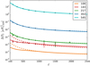 |
Fig. 1. Angular power auto-spectra of the clustered CIB component used in simulations. The dashed lines represent the 1D clustered CIB spectra obtained by fitting data points to a polynomial at 545 GHz and scaling this template to lower frequencies. The solid lines represent the ND clustered CIB obtained by separately fitting data points at each frequency. Overplotted data are taken from Table D2 of Planck Collaboration XXX (2014). No data points are available for the 100 GHz clustered spectrum, which is taken to be one order of magnitude less than the 143 GHz clustered spectrum. Spectra have been corrected for shot-noise contribution in order to match data points. |
– SET2: these simulations include one foreground source which is not fully coherent across frequencies. Galactic dust and the two point-source populations are each simulated as a 1D template rigidly scaled through frequency (refer to Table 1 for point sources) but the clustered CIB presents frequency decoherence, that is,
 (21)
(21)
where the coefficients αν1 × ν2 ≤ 1 are taken from Planck Collaboration XXX (2014) and are reported in Table 2. The angular power spectrum shape is modelled on observational estimates: its shape varies with frequency, as shown in Fig. 1. We refer to this CIB component as ND or multidimensional.
Decoherence coefficients for the ND clustered CIB.
– SET3: these simulations have the most realistic foreground content. The two point-source populations are each simulated as a 1D template rigidly scaled through frequency (again refer to Table 1). The clustered CIB is simulated as in SET2. The dust component presents spectral index and dust temperature variability on the sky, using results from Planck Collaboration XLVIII (2016). We refer to this dust component as ND or multidimensional.
These three sets are labelled SET1, SET2, and SET3 throughout this work. The SET2 and SET3 cases are studied since observations show that there could be a partial decoherence through frequency of the CIB emission (Planck Collaboration XXX 2014, Sect. 6.2), this effect being mostly evident at the two lowest frequencies, 100 and 143 GHz. SET3 case also includes a realistic dust representation, which takes into account the inhomogeneous dust properties on the sky. Both are important tests since the SMICA method assumes no frequency decoherence or variability of the spectral index for the one-dimensional sources; in the SMICA model this variability is accounted for as an increase of the dimensionality of the source. However the model has a maximum number of dimensions fixed by the number of observations.
In order to reproduce the Planck half-mission maps used in this analysis, for each simulation we produce two maps for each frequency, with identical astrophysical content but differing in their realisation of white Gaussian noise. We produce N = 30 simulations for each set.
Building the components. The CMB component is simulated from a theoretical CMB temperature angular power spectrum using the HEALPix tool (Górski et al. 2005). The power spectrum is obtained using the code CAMB (Lewis & Bridle 2002), with the following set of input cosmological parameters: H = 67.31, τ = 0.078, ωb = 0.02222, ωc = 0.1197, ns = 0.9655, ln(1010As) = 3.089, yHe = 0.24 and mν = 0.06 eV.
There are two different thermal dust components: one is a single template scaled through frequency (SET1 and SET2 simulations), while the other presents more complex features (SET3). The former, labelled “1D”, is the thermal dust map at 545 GHz delivered by the Planck collaboration (Planck Collaboration X 2016), which we choose in order to have a realistic spatial distribution. This template is scaled through frequency according to the grey-body law described by Eq. (1) with T = 19.4 K and β = 1.6 (Planck Collaboration XLVIII 2016). We note that this template is partially contaminated by residual CIB emission (Planck Collaboration X 2016, Sect. 4), which makes the dust contribution of this template at high ℓ higher than the real dust contribution. This makes the fit of the high-ℓ components slightly more difficult for SMICA. Due to the fact that thermal dust and the clustered CIB have similar emission laws, the presence of a residual contamination of CIB in the small scales of the thermal dust template map is not to be excluded, that is, the small-scale power of this template could be higher than the real dust distribution. The latter, labelled “ND”, is simulated using the GNILC model maps for the spectral index βd, the dust temperature, and the opacity, obtained as described in Planck Collaboration XLVIII (2016). They are combined through Eq. (1) to produce a dust map at each ν.
For the extragalactic content, that is, point sources and clustered CIB, we base our analysis on Planck Collaboration XXX (2014), which provides estimates for the radio and IR point-sources shot-noise levels, the angular power spectra of CIB emission, and its decoherence coefficients at Planck frequencies. Shot-noise levels are given at all the frequencies of interest of this paper, and we therefore use them for point-source simulations. We model the two point-source populations as two realisations of shot-noise maps, that is, with a flat angular spectrum. The amplitudes of the shot noise power are taken from Tables 6 and 7 in Planck Collaboration XXX (2014) and are summarised in Table 1.
The CIB spectra and decoherence coefficients are given by the Planck analysis for all frequencies except 100 GHz: for this channel, we choose values one order of magnitude lower than the 143 GHz estimates. The CIB angular power spectra reported in Table D2 of Planck Collaboration XXX (2014) contain both the clustered and shot-noise contribution: the latter is subtracted to obtain clustered CIB templates. To produce the clustered CIB component maps at each frequency we compute the covariance matrix  of CIB auto- and cross-angular power spectra. More specifically, for SET1, that is, the 1D clustered CIB, we fit a polynomial to the data points of the 545 GHz power spectrum, and all the other auto- and cross-spectra are obtained by scaling this template. Scaling coefficients for auto-spectra are obtained from Planck Collaboration XXX (2014), while for cross-spectra we use Eq. (21) with αν1 × ν2 = 1. Cℓ = 3000 values are reported in Table 1. Whereas for SET2 and SET3, that is, the ND clustered CIB, at each frequency we fit a polynomial to the data points of the auto-spectra given in Planck Collaboration XXX (2014), and we extrapolate to higher ℓ when necessary. Only the auto-spectra are used, while cross-spectra are derived via Eq. (21). The decoherence coefficients of angular power spectra between different frequencies are detailed in Table 2.
The auto-spectra for both cases are presented in Fig. 1. Once the covariance matrix  is constructed, the procedure for obtaining spherical harmonics is the same for both cases. We build the vector xℓm, whose entries
  are sets of spherical harmonics coefficients drawn from the normal distribution,
 (22)
(22)
where i = 1, 2, …N, and N is the number of frequencies we use. We then obtain spherical harmonics for the CIB as
 (23)
(23)
where  is the square root of the clustered CIB covariance matrix
  . In order to build simulations, the CMB and foregrounds maps are added with their respective amplitude for each frequency and then smoothed with their respective beam window function3. By construction, there is no correlation between the foregrounds and the CMB.
The instrumental noise is simulated at the map level as white Gaussian noise. The noise rms for each map is constant over the sky at a value determined from the Planck noise simulations (provided at NERSC4).
4.2. Planck data
We use data maps from the 2015 full Planck release. We select the two half-mission maps at each frequency between 100 and 545 GHz. Half-mission maps are data split obtained by dividing the full mission time-ordered data into two halves. The maps are degraded to a lower resolution of Nside = 1024 using HEALPix.
4.3. Masks and binning
In order to reduce the foreground contamination, the central regions of the sky are masked. Masks are produced as the sum of a galactic and a point-source part. We use a set of three masks with the same point-source masking but different galactic coverage. The masks used are shown in Fig. 2 and have effective fsky = 0.3, 0.5, and 0.6. More details on preparation of the masks are given in Appendix A.
 |
Fig. 2. Apodised masks used in this analysis. The retained sky fractions fsky = 0.3, 0.5, 0.6 are shown in red, green, and blue, respectively. The shaded region is the apodised part. |
SMICA works with spectral covariance matrices, and angular power spectra between all pairs of maps are calculated with the PolSpice (Chon et al. 2004) package. Using the PolSpice routine, we correct the resulting power spectra for the pixel window function, for the mask leakage, and for the point spread function of the instrument using the beam window functions provided by the full Planck release[3]. All the angular power spectra are binned uniformly with Δℓ = 15. With these spectra, and following the procedure detailed in Sect. 3.2.1, we build at each bin a 5 × 5 covariance matrix  . We work on the range ℓ = [100, 2500]; we neglect in this analysis the large angular scales ℓ < 100, where dust has complex features that cannot be described by a bidimensional component. Also, we limit our analysis around ℓ ∼ 2500, since noise becomes dominant for higher multipoles.
The Planck maps are slightly decalibrated among one another. Similarly to what is done in the Planck analysis (Planck Collaboration XII 2014), we perform a dedicated free fit in the multipole range of the first and second peaks to recover calibration factors. We use relative calibration correction factors with respect to 143 GHz: ycal=[1.00079, 1., 1.0029, 1.008, 1.0174] for the five channels between 100 and 545 GHz.
5. Testing the method
We detail here the analysis and fitting procedure to obtain the CMB power spectrum. We test this method first on simulations and then on Planck 2015 temperature data. The spectra recovered from simulations and data are used to estimate cosmological parameters, which are presented in Sect. 6.
5.1. Simulations analysis
While the simulated foregrounds cannot reproduce the full complexity of real data foregrounds, a study on simulations is a good test for elucidating the accuracy to which we can recover the point source signal and the CMB angular power spectrum. We process the three simulation sets with the foreground model described by Eq. (20). Since foregrounds are all 1D, for SET1 we constrain the  component to be diagonal.
In the top panel of Fig. 3 we show the recovered shot-noise point-source signal for the average of all simulations of each set at fsky = 0.5. We show results for the intermediate fsky value, but we observe no mask dependence in the recovered point-source emission. We observe that the model is capable of recovering closely, up to small offsets, the point-source input for all three cases. The SET1 case, which has all 1D foregrounds and is therefore an ideal test case for SMICA, presents a small offset in the three central frequencies, even though the foreground content corresponds exactly to the SMICA model. This is not surprising, as the clustered CIB, the IR shot-noise, and the galactic dust have similar emission laws, and the corresponding columns of the matrix A are almost proportional, as seen in Fig. 4. This is far from ideal for ICA methods, since it limits the identifiability of the sources. Due to this, we expect an exchange in power between dust, cCIB, and IR point sources. The offsets in SET2 and SET3 simulations are instead likely due to the fact that the model is incapable of representing the foregrounds complexity due to its limited dimensionality.
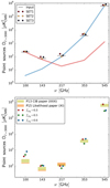 |
Fig. 3. Combined (IR and radio) shot-noise point sources Dℓ power at ℓ = 3000 obtained from the fit. Top panel: simulations average of point sources at fsky = 0.5, shown in dark red for SET1 simulations, yellow for SET2, and black for SET3. The red and blue bands show the simulations input for the radio and IR point sources, respectively, while the grey horizontal line at each ν represents the joint point-source input. Bottom panel: point sources for the three different masks of fsky = 0.6, 0.5, 0.3 in blue, green and red, respectively. The yellow and orange bands represent the expected shot-noise point-source contribution estimated in Planck Collaboration XXX (2014) and Planck Collaboration XI (2016), where the width of the coloured band represents the error on the expected value. Planck Collaboration XI (2016) gives expected values for the three low ν channels only. |
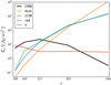 |
Fig. 4. Input spectral behaviour of dust, clustered CIB, IR, and radio point sources of SET1 simulations at fsky= 0.5, plotted as Cℓ = 3000. Radio and IR point sources are labelled “rad” and “ir”, respectively. Infrared point sources, cCIB, and dust, plotted in blue, green, and orange, respectively, present similar emission laws. The CMB black-body emission law, which is not fitted for, is plotted in black. |
In the left panel of Fig. 5 we show residuals of the high-ℓ tail of the fitted CMB angular power spectrum with respect to the theoretical input. As seen from this figure, the residual is at most one fifth of the CMB power at ℓ ≥ 2200. A residual contamination is present on average for the SET2 and SET3 cases only. The misevaluation of the clustered CIB contamination can be one source of bias in the CMB power spectrum estimation. The SMICA method assumes full correlation of all components through frequency. A partial decoherence of a component, as for example in SET2 for the clustered CIB, means that its spectral behaviour must be described by a multidimensional component. For galactic dust and clustered CIB, we have a 2D component describing both of them at the same time. While angular power spectra are fitted in each bin, the mixing matrix A is global: galactic dust and clustered CIB emissions, which are important at low and high multipoles, respectively, compete for the columns of this matrix. As a consequence, complex features in these two emissions cannot be fully accounted for. We expect that a part of the CIB and dust contamination is projected onto the CMB, resulting in an offset with respect to the input spectrum, as shown in the left panel of Fig. 5.
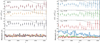 |
Fig. 5. Top three panels: residuals in Dℓ between the fit results and the theoretical CMB power spectrum. The dark grey line shows the theoretical CMB spectrum downscaled by a factor of 0.2 for readability. Bottom panel: mismatch between the model and the data after the fit as defined by Eq. (3.1) and the thin dashed line shows the expected mismatch per bin. Only one point every three bins is displayed. Left panel: filled dots show differences between CMB spectra obtained from fit on simulations with respect to input CMB spectrum at each bin, at fsky = 0.5, shown in dark red for SET1, yellow for SET2, and black for SET3. Right panel: filled dots show differences between CMB spectra obtained from the fit on Planck 2015 half-mission data and the Planck best fit ΛCDM Plik spectrum. |
We can see that such a contamination is not detectable as a considerable increase in the mismatch, while it is clearly visible in the CMB residuals. Results in Fig. 5 are presented for fsky = 0.5, but no significant trend with sky fraction is visible in most simulations. We see that the observed mismatch is lower than the expected value. This happens because of the peculiar statistical properties of the empirical covariance matrices used in this work, as described in Sect. 3.2.1. The value of the mismatch does not correspond to the number of degrees of freedom ν, which we plot anyway as a visual reference of the order of magnitude of the expected mismatch (see Sect. 3.1 for more details).
5.2. Data analysis
We fit a model as described in Sect. 3.3. The obtained CMB angular power spectrum is presented in Fig. 6 for the three different masks, while the right panel of Fig. 5 shows residuals with respect to the reference CMB Planck spectrum at high-ℓ. The reference Planck spectrum is the theoretical ΛCDM spectrum obtained from best fit parameters of the Planck 2015 Plik likelihood exploration. Error bars are derived with the Fisher matrix.
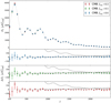 |
Fig. 6. CMB angular power spectrum obtained from the SMICA fit of the model to the three different data sets used, corresponding to the masks with fsky= 0.3, 0.5, and 0.6 (top panel). In grey we show the best fit theoretical ΛCDM spectrum obtained with Plik. The three bottom panels show the residuals between theory and data for the three cases, together with the theoretical value of the angular power spectrum scaled to 20% power in grey. The black dashed line shows the total contribution of extragalactic foregrounds at 217 GHz. To enhance readability, only one point in four is plotted. |
We observe in Fig. 5 that the results obtained for the CMB are in good agreement between the three different masks. For increasing sky fraction, we can see an increasing level of residual contamination. While this trend is not seen in simulations, we expect such a behaviour in real data since the foreground complexity increases. As observed in simulations, we expect that the model cannot fully capture dust and cCIB emission. Also, our simulations contain two point-source populations perfectly correlated through frequency. While this is a good approximation, it might not represent the full extent of contamination produced by background galaxies. Another problem is the similar emission law between dust and CIB, which cannot be fully captured by the model; due to this, a fraction of the foreground contamination projects onto the CMB and onto the mismatch between the model and the data. We see that the mismatch is much higher than the mismatch found in simulations, in particular for the smallest mask and at low multipoles, where the thermal dust behaviour becomes more complex.
In the bottom panel of Fig. 3 we show the recovered point-source amplitudes for the three masks at ℓ = 3000. Results for fsky = 0.3, 0.5 are in good agreement with each other and with the expected amplitude as estimated by the Planck collaboration. The fsky = 0.6 results show an offset at the highest and lowest frequencies: again, the model fails to fully represent the complexity of the foregrounds. We expect point-source estimates at smaller fsky to be more accurate, since the galactic contamination is lower. The offset of point-source emission law is related to the offset in the CMB power spectrum, but cannot fully explain it. Forcing point-source emission law to the result obtained for the largest mask, that is, to a value closer to the expected one, only slightly reduces the mismatch and the CMB bias.
5.3. Using 857 GHz
The number of channels used is directly related to the dimensionality of the foreground model. Including more observations allows for a higher dimension, but also adds new features in the data that need to be described. We choose to exclude low-frequency observations from our analysis since this would include synchrotron and free–free emission and thus increase the Galactic foreground complexity. We also choose to exclude WMAP 94 GHz observations since they have a lower resolution than Planck data and this would oblige us to use a smaller ℓ range.
Higher frequency observations could in principle be useful since they contain mainly dust, IR point sources, and clustered CIB. However, frequency decoherence of foregrounds makes the effective impact of high-frequency channels negligible. We present in this section results on SET3 simulations and Planck data when adding the 857 GHz channel. For the analysis on data, the masks are adapted by adding point sources detected in the 857 GHz maps, but effective sky fractions are substantially unchanged. The fitting procedure is the same as described in Sects. 5.1 and 5.2, with the only difference being that the  part of the model in Eq. (20) now has three dimensions instead of two.
For simulations, we see no evident difference in the SMICA fit between adding the 857 GHz channels or not. For data, the CMB power spectrum for fsky = 0.5, 0.6 is shown in Fig. 7. In this case, no improvement is seen with respect to the fit without the 857 GHz channel. At high ℓ, residuals are lower when this channel is excluded. Also, while simulations show good agreement between masks, the recovered point-source emission laws for data show an evident bias at low frequencies ν ≤ 217 GHz. This suggests that a degree of decoherence is present between 857 GHz and lower-frequency shot-noise emission. The mixing matrix columns reserved to point sources cannot accommodate for both high and low frequencies, sacrificing the latter.
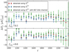 |
Fig. 7. CMB angular power spectrum Dℓ residuals with respect to Planck theoretical best fit spectrum for three different SMICA configurations. In blue we show the leading configuration of this paper using cross-spectra of data splits, in red the one using cross- and auto-spectra as described in Sect. 5.4, and in green the results obtained including 857 GHz channel observations, as detailed in Sect. 5.3. Only one point every three bins is displayed. We show results for fsky = 0.5 in the top panel and fsky = 0.6 in the bottom panel. We note that the baseline analysis of this paper (red), i.e. the case which uses |

5.4. Without data splits
The configuration described in Sect. 3.2.1 tests covariance matrices built using data-split cross-spectra only. A simpler configuration would be to use the full 2N × 2N covariance matrix of auto- and cross-spectra, where N is the number of frequency channels. This matrix is defined as
 (24)
(24)
where ![Mathematical equation: $ \boldsymbol{y}_{\ell,m}^{\mathrm{full}}= [\boldsymbol{y}_{\ell,m}^{a},\boldsymbol{y}_{\ell,m}^{b}] $](/articles/aa/full_html/2019/04/aa33758-18/aa33758-18-eq49.gif) . The model used in this case is
. The model used in this case is
 (25)
(25)
where Nℓ is the diagonal matrix containing the noise power spectra. In this configuration the noise power spectra are part of the fitted parameters. This higher number of parameters to fit is compensated for by the increased dimension of the data matrix R̂ℓ.
In regards to Planck data, we show in Fig. 7 that residuals for the cross-spectra-only covariances R̂ℓ are lower than those obtained using the auto- and cross-spectra covariances  . We attribute this difference to the higher number of parameters to fit in the full matrix case. Also, an error in the noise estimation reflects on the astrophysical part of the fit, and potentially on the CMB. Instead, in the configuration chosen for this study, noise spectra are known by construction and are not fitted for, and thus they cannot bias the fit. The drawback in this case is that the estimated error bars depend on the noise ansatz (see Sect. 3.2.2).
6. Cosmological parameters
We test our approach by obtaining cosmological parameters from the SMICA best-fit angular power spectrum. We do this both for Planck data and for a subset of simulations. We compare the parameters obtained from simulations to the input ones. The parameters obtained from Planck data are compared to the baseline Planck 2015 results. Since we only have temperature data, we use a Gaussian prior on the parameter τ: this configuration in Planck Collaboration XI (2016) is referred to as PlikTT+tauprior. For each case studied, we run Monte Carlo Markov chains (MCMC) with CosmoMC (Lewis & Bridle 2002) in combination with PICO5 (Fendt & Wandelt 2007). We also cross-check some of our runs using CosmoMC with CAMB, and using CosmoSlik (Millea 2017) with PICO. We observe that results are consistent with those obtained using CosmoMC with PICO, with differences of the order of 0.1σ on average. For this reason, all the results presented in this analysis are obtained using the latter configuration.
6.1. The likelihood
We build our likelihoods from the best-fit CMB spectra obtained from the SMICA fit for the different cases under analysis. We use an idealised form for the likelihood, which considers no intermode correlations. This approximation should not strongly affect our results since we use bins of Δℓ=15. The likelihood takes the form
 (26)
(26)
where Ĉ and C(θ) are the best fit and theoretical angular power spectra, respectively, Σ is the covariance matrix given by the SMICA error bars on the best fit, and c is a constant. The error bars are an estimate derived from the Fisher matrix. They represent the cosmic variance, foregrounds, noise and mask contribution to the error budget, but do not include uncertainties on calibration and beams.
We explore a minimal ΛCDM model with two approximately massless neutrinos and one massive neutrino with ∑mν = 0.06 eV. We also use a Gaussian prior on the optical depth to reionization: for the MCMC on data we use τ = 0.07 ± 0.02, the same as in Planck analysis (Planck Collaboration XI 2016), while for simulations we choose τ = 0.078 ± 0.02, since τ = 0.078 corresponds to the input value of the simulated CMB maps.
There is a small amount of foreground residuals in the CMB spectra, as evident from Fig. 5. This residual has to be accounted for in the likelihood formulation with a nuisance model. Finding a shape for the foreground residuals is not trivial, since nuisance parameters can bias the cosmological parameters when incorrectly chosen. We opt for a physical modelling of the nuisance parameters based on our foreground knowledge. Paoletti et al. (2012) find that two terms for the shot noise and clustered contribution suffice to account for the contribution from background galaxies. Also, we need to account for residuals of the galactic dust. We do not consider any term for the SZ residual contamination.
The Planck collaboration derives cosmological parameters from the CMB maps, including the SMICA one (Planck Collaboration IX 2016). The cosmological parameters of the SMICA map cannot be directly compared to these analysis parameters since the map-making procedure can add some foreground contribution. We therefore compare our results with those obtained with the Planck likelihood, which uses angular power spectra of data maps. Nevertheless, similarly to the Planck analysis on CMB maps, we use a nuisance model that comprises three terms:
-
a point-source term with flat spectrum. Its amplitude is regulated by the parameter APS, which corresponds to the point sources contribution for Dℓ = 3000;
-
a clustered CIB term with a spectrum ℓnCIB. We fix nCIB = −1.3 for most explorations, unless otherwise stated. The amplitude ACIB represents the CIB contribution for Dℓ = 3000;
-
a dust term with an angular power spectrum ℓ−2.6. The nuisance parameter Adust is defined as the emission for Cℓ = 500.
The physical nuisance model is our reference configuration. We test a subset of configurations using a smaller number of nuisance parameters, as well as the use of a single template derived from simulations. The template is based on the shape of the average foreground residuals in SET3 simulations at the largest fsky, that is, the case with the strongest residual contamination in the CMB spectrum. Its shape does not represent any particular foreground contamination, however it is very close to the clustered CIB theoretical shape, meaning that this is the major contribution that we expect in the residuals according to simulations. Figure 8 shows the difference between the best fit CMB spectrum and the spectrum of the input CMB map for ten SET3 simulations. The input maps are unmasked, and therefore the low-ℓ scatter is largely driven by cosmic variance. From these we compute the average residuals and fit a shape for the template. We use this template as a unique nuisance component in the likelihood exploration, only changing its amplitude.
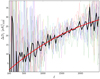 |
Fig. 8. Difference between SMICA best fit and input maps CMB angular power spectra for ten SET3 simulations. The average of the differences is plotted in black, while the chosen template for the likelihood is plotted in red. |
6.2. Cosmological parameters from simulations
We explore cosmological parameters for the first ten simulations of each set. For these simulations, we obtain parameters for both the largest and the smallest masks to check for effects that depend on retained sky fraction. For each simulation and sky fraction, we use the best fit CMB angular power spectrum of SMICA to build a likelihood as described in the previous section. The main analysis is done using the physical parametrisation of the nuisance model. The list of all parameters is detailed in the first column of Table 3. Cosmological parameters are presented in Fig. 9 for SET1 and Fig. 10 for SET2 and SET3, where the red line shows simulation inputs and the wide coloured band shows 1σ scatter of the marginal mean values.
Results of the MCMC exploration with the three considered likelihoods: Like-F03, Like-F05, and Like-F06.
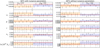 |
Fig. 9. Cosmological parameters for a subset of ten simulations of SET1 with (left panel) and without (right panel) a model for nuisance parameters in the likelihood. Results are presented for fsky = 0.3 in yellow and fsky = 0.6 in blue. For each fsky, the dashed line represents the average of the marginal means of the simulations and the shaded band represents the 1σ scatter around this average. Each dot represents the marginal mean and 68% CL error bar of the parameters in a given simulation. The red line shows the input parameters of theoretical Cℓ used for simulations. |
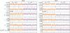 |
Fig. 10. Cosmological parameters for a subset of ten simulations of SET2 (left panel) and SET3 (right panel). Results are presented for fsky = 0.3 in yellow fsky = 0.6 in blue. For each fsky, the dashed line represents the average of the marginal means of the simulations and the shaded band represents the 1σ scatter around this average. Each dot represents the marginal mean and 68% CL error bar of the parameters in a given simulation. The red line is the input of theoretical Cℓ used for simulations. |
The SET1 simulations best recover the input CMB power spectrum in the SMICA fit, and therefore we expect their residual foreground content to be very low. We test SET1 simulations in two different configurations, leaving the nuisance parameters free and setting all of them to zero, that is, not accounting for any residuals in the likelihood exploration. As shown in the right panel of Fig. 9, the MCMC exploration with nuisance parameters shows evident biases with both masks. As a cross-test, we obtain cosmological parameters from theoretical spectra to which we add some scatter according to the expected cosmic variance. In this case the average parameters obtained coincide with the input. This means that the shift we observe in Fig. 9 is due to foreground residuals and not to our pipeline implementation.
As we see in Sect. 6.3, there is a degeneracy between the shape of the foreground residuals and the cosmological parameters, and an incorrect estimation of the nuisance parameters can induce biases. In particular, when we have a low fsky, the error bars are larger and we can more easily mix up the CMB and the foregrounds. This is evident in Fig. 9, which shows how most biases are strongly reduced when nuisance parameters are removed, especially for fsky = 0.3, where we expect to have the lowest, and therefore most degenerate residuals. Due to the low level of residuals in the CMB spectra, the nuisance parameters are not well estimated and are in most cases compatible with zero. A level of residuals is present in the data, but since this is not well determined, it is not correctly accounted for.
For SET2 and SET3 simulations, we obtain less biased results: in Fig. 10 we can see that biases of parameters are less evident, especially for the SET3 case. In this case we did not run the nuisance-free likelihood, given that the level of foreground residuals is too high to justify such a test. Since the level of residuals in these simulations is higher than in SET1, it is better constrained in the parameters exploration. We observe very small changes with sky fraction, the most relevant one being the decrease in size of the 1σ scatter band with increasing fsky, as expected. We note that marginal errors on τ and As for individual simulations are relatively large, while the scatter of the mean is not; this is not surprising since the marginal error on τ, and consequently on As, is regulated by the Gaussian prior τ = 0.07 ± 0.02 we impose.
Since the nuisance parameters are not well constrained, a model for the residuals with less parameters could in principle reduce the uncertainty in the exploration. For the SET3 case only, we test the template configuration of the likelihood described in the previous section. In this configuration, only one nuisance parameter is fitted, which is the amplitude of the template. In terms of biases, the results are equivalent to those obtained with the physical nuisance model. The only relevant change is that the discrepancy on As is reduced, while that on ωb is increased. This suggests that the average foreground contamination represented by the template does not fully describe the details of the residuals in each CMB spectrum of simulations, and that the details of foreground modelling in the likelihood are important for accurate estimation of cosmological parameters.
6.3. Cosmological parameters from Planck data
We build a likelihood for each mask from best fit spectra obtained from the analysis detailed in Sect. 5.2. We call these three likelihoods Like-F03, Like-F05, and Like-F06, where FX refers to the fsky of the mask used. We run an MCMC exploration with Planck high-ℓ temperature likelihood and compare the results with those published by the Planck collaboration. We find good agreement between these two runs of the Planck likelihood, that is, within less than 0.1σ. We interpret this as confirmation that our configuration is the same as that used for the Planck analysis.
We give results for our three likelihoods and compare them to the Planck likelihood run. We note that a Gaussian prior is imposed on the absolute map calibration for Planck likelihood ycal = 1 ± 0.0025, while we keep this value fixed to ycal = 1. We adopt this choice after verifying that including this parameter in the explorations does not affect the results, apart from increasing the total number of parameters to be sampled.
We plot a comparison of the cosmological parameters estimated in Fig. 11, while the full list including derived parameters can be found in Table 3. The respective values for the Planck likelihood analysis can be found in Planck Collaboration XI (2016), where Table 17 lists the cosmological parameters and Table 10 the nuisance parameters. Shifts of cosmological parameters in units of 1σ Planck error bars are presented in Table 4: for most parameters we observe a progressive shift increasing with the retained sky fraction, the most evident case being for ns. On the whole, parameters show at most 1σ deviation with respect to the Planck analysis, with the only exception of ωb for fsky = 0.3, which shows a deviation of −2.04σ, and ns for fsky = 0.6, which shows a deviation of 1.48σ.
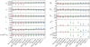 |
Fig. 11. Marginal mean and 68% CL error bars for cosmological parameters obtained with Like-F03 in red, Like-F05 in green, and Like-F06 in blue. For comparison, Planck 2015 high-ℓ temperature likelihood results are shown in the background, with the marginal mean drawn in black and 68% CL represented by a grey band. On the left we show the six standard ΛCDM cosmological parameters and on the right some derived and nuisance parameters. Nuisance parameters show no Planck comparison since they are specific to the likelihood. The values of nuisance parameters are in units of μK2. The template amplitude is shown in the ACIB column since its shape is very close to that of the CIB term in the nuisance physical model. |
Shift of parameters between the three data likelihoods Like-F03, Like-F05 and Like-F06 and the Planck high-ℓ likelihood results in units of 1σ Planck errors.
At low fsky the residuals are weak and not clearly constrained by the nuisance model. As seen in simulations, there is an uncertainty in the value of the nuisance parameters that induces a shift in the cosmological parameters. In Fig. 12 we can see that nuisance parameters are consistent with zero and are also strongly degenerate among them. Some degeneracies are also visible with the cosmological parameters, as for example between Ase−2τ and Adust. Due to the strong correlation between all cosmological parameters, these degeneracies can induce biases. Also, as noted by Huffenberger et al. (2006), the parameter ns is particularly sensitive to incorrect subtraction of the point source component, since a residual of point sources can mimic a different tilt of the CMB angular power spectrum. The biases we obtain are representative of the uncertainty on the determination of the foreground model.
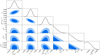 |
Fig. 12. Triangle plot showing the relation between the main cosmological parameters and the nuisance parameters for the analysis of data with fsky = 0.6. Similar plots are obtained for SET3 simulations and for different fsky. The blue and light-blue contours represent the 68% and 95% CL, respectively. |
For Like-F03, we perform an analysis without any nuisance parameters, finding smaller shifts with respect to the reference configuration. This is further evidence for the existence of degeneracies between cosmological and weakly constrained nuisance parameters. Results are shown in the “No nuisance” column of Fig. 11. This analysis is only possible for fsky = 0.3 since the level of residuals is too high for the other two masks.
The results of the analysis using a template are also shown in Fig. 11. This configuration performs slightly better, especially at low fsky, reducing the biases on ns and ωb. No significant improvement is seen however at high fsky. Furthermore, the total foreground power detected by the template is lower at fsky = 0.6 than at fsky = 0.5. This suggests that for a high sky fraction the template is no longer representative of the residual contamination in the CMB spectrum. This is partially true also for the physical nuisance model, meaning the residuals at large sky fraction are not well represented by either model.
We note that the biases observed in the data analysis are different from those observed in simulations. This suggests that the foreground complexity is not well accounted for in our simulations and that the correct choice of the nuisance model strongly depends on the details of the foreground contamination.
6.4. Cross-tests on data
Results presented in Tables 3 and 4 refer to the main exploration detailed above. As a cross-check Fig. 11 shows the results of two different configurations. The first uses best-fit CMB spectra as obtained from Sect. 5.4, where both auto- and cross-spectra are used to build covariance matrices. The second adds the CIB index as a nuisance parameter, which defines the angular power spectrum shape of the CIB residuals as ℓnCIB. This parameter is varied with a Gaussian prior nCIB = −1.3 ± 0.2. We observe no relevant shift in the obtained cosmological parameters from these two additional configurations.
We also obtain cosmological parameters from the best fit obtained using the 857 GHz channel as described in Sect. 5.3. We run MCMC for fsky = 0.6 on SET3 simulations and obtain cosmological parameters which are consistent with those shown in Fig. 10 within a maximum of 0.022σ (σ here is the scatter of the marginal mean among various simulations). Conversely, on the Planck data analysis, cosmological parameters are more strongly biased than those obtained without the 857 GHz channel, in particular ns and ωb. While the increase in foreground residuals in the spectrum is modest, we expect their characteristics to be quite complex and not adjustable by the minimal nuisance model that we use.
7. Conclusions
We have studied a new configuration of the SMICA method to estimate the CMB angular power spectrum directly via component separation. This configuration uses only cross-angular power spectra between half-mission data split, thus avoiding the noise bias present in auto-spectra. We use a constrained foreground model that targets the extragalactic point-source emission. This is particularly important since the level of point sources is degenerate with the CMB at small scales. For the CMB power spectrum, we use SMICA to jointly fit the point sources emission law and other foreground angular spectra and frequency emission, such as dust and clustered CIB.
We obtain an estimate for the point-source emission law that is consistent with independent estimates of the Planck collaboration analysis. We recover a fit of the CMB angular power spectrum that we use to derive cosmological parameters through an MCMC likelihood exploration, using both Planck 2015 data and simulations. To model the foreground residuals in the CMB spectra, two configurations of nuisance parameters are studied: a physical model and an artificial template based on results of simulations. In both cases the cosmological parameters we obtain for simulations and Planck data agree with the predicted values of the Planck collaboration analysis (Planck Collaboration XIII 2016) within 1σ on average. The level of biases that we observe on the simulations shows us the level of bias expected in the real data.
The observed shifts strongly depend on the foreground residuals and on the nuisance model of the likelihood. If the foreground residuals are weak, the nuisance parameters are not well constrained by the data, and their misevaluation can induce biases on the cosmological parameters. When the foreground contamination is stronger the foreground model is better constrained and the biases are reduced. However the characteristics of the residuals need careful modelling, and a minimal model, as used in this work, is not sufficient to describe them. We observe this when analysing either simulations or Planck data. Using a single foreground template for nuisance conveys the advantage of having less parameters to fit. However the shape of this template is not universal and again it depends on the characteristics of the foregrounds.
In conclusion we observe that a blind method such as SMICA with an adapted model for the extragalactic foregrounds can recover an estimate of the CMB power spectrum which has a very low foreground residual content. However, in order to use this estimate for cosmological purposes, extensive knowledge and careful modelling of the shape of the foreground residuals are needed. The same is also true for the Planck likelihood analysis in Planck Collaboration XV (2014). Therefore, it is not clear whether this blind approach grants any advantage, at least for the CMB temperature analysis, where foregrounds are particularly complex. When considering polarization, a blind approach could still be useful since the small-scale foreground contamination is more simple, while SMICA has demonstrated its ability to deal with large-scale complex contamination (Planck Collaboration XII 2014). Also, using a zone approach with SMICA that would take into account the variability of galactic foregrounds on the sky could improve the efficiency of component separation and thus improve estimations of cosmological parameters.
We use real valued spherical harmonics.
Nevertheless, for our configuration, simulations show that it is of the same order of magnitude as d.
Provided in Planck’s RIMO (reduced instrument model), which can be downloaded from the Planck Legacy Archive http://pla.esac.esa.int/pla/
Available for download at https://github.com/marius311/pypico
Available for download at http://pla.esac.esa.int (HFI_Mask_GalPlane-apo0_2048_R2.00.fits)
v2.0, also available for download at http://pla.esac.esa.int
Acknowledgments
UC wishes to thank Aurélien Benoit-Lévy for suggestions on masks treatment, Silvia Galli for discussions on simulations and cosmological parameters, Éric Hivon for tips on the use of HEALPix, Marius Millea for helpful insight on radio point sources, and CosmoSlik and Mario Ballardini for helpful suggestions on CosmoMC. This work has made use of the Horizon Cluster hosted by Institut d’Astrophysique de Paris. We thank Stephane Rouberol for running smoothly this cluster for us. UC has been supported within the Labex ILP (reference ANR-10-LABX-63) part of the Idex SUPER, and received financial state aid managed by the Agence Nationale de la Recherche, as part of the programme Investissements d’avenir under the reference ANR-11-IDEX-0004-02. This research used publicly available Planck data.
References
- Basak, S., & Delabrouille, J. 2012, MNRAS, 419, 1163 [NASA ADS] [CrossRef] [Google Scholar]
- Basak, S., & Delabrouille, J. 2013, MNRAS, 435, 18 [NASA ADS] [CrossRef] [Google Scholar]
- Bedini, L., Herranz, D., Salerno, E., et al. 2005, EURASIP J. Appl. Sign. Proces., 2005, 2400 [NASA ADS] [CrossRef] [Google Scholar]
- Bobin, J., Moudden, Y., Starck, J.-L., Fadili, J., & Aghanim, N. 2008, Stat. Methodol., 5, 307 [NASA ADS] [CrossRef] [Google Scholar]
- Bobin, J., Starck, J.-L., Sureau, F., & Basak, S. 2013, A&A, 550, A73 [NASA ADS] [CrossRef] [EDP Sciences] [Google Scholar]
- Bonaldi, A., Bedini, L., Salerno, E., Baccigalupi, C., & De Zotti, G. 2006, MNRAS, 373, 271 [NASA ADS] [CrossRef] [Google Scholar]
- Cardoso, J. F. 2017, in Latent Variable Analysis and Signal Separation, eds. P. Tichavský, M. Babaie-Zadeh, O. J. Michel, & N. Thirion-Moreau (Cham: Springer International Publishing), 403 [Google Scholar]
- Cardoso, J.-F., Le Jeune, M., Delabrouille, J., Betoule, M., & Patanchon, G. 2008, IEEE J. Sel. Top. Sign. Proces., 2, 735 [CrossRef] [Google Scholar]
- Chon, G., Challinor, A., Prunet, S., Hivon, E., & Szapudi, I. 2004, MNRAS, 350, 914 [NASA ADS] [CrossRef] [Google Scholar]
- Delabrouille, J., Cardoso, J.-F., & Patanchon, G. 2003, MNRAS, 346, 1089 [NASA ADS] [CrossRef] [Google Scholar]
- Delabrouille, J., Cardoso, J.-F., Le Jeune, M., et al. 2009, A&A, 493, 835 [NASA ADS] [CrossRef] [EDP Sciences] [Google Scholar]
- Eriksen, H. K., O’Dwyer, I. J., Jewell, J. B., et al. 2004, ApJS, 155, 227 [NASA ADS] [CrossRef] [Google Scholar]
- Eriksen, H. K., Jewell, J. B., Dickinson, C., et al. 2008, ApJ, 676, 10 [NASA ADS] [CrossRef] [Google Scholar]
- Fendt, W. A., & Wandelt, B. D. 2007, ArXiv e-prints [arXiv:0712.0194] [Google Scholar]
- Fernández-Cobos, R., Vielva, P., Barreiro, R. B., & Martínez-González, E. 2012, MNRAS, 420, 2162 [NASA ADS] [CrossRef] [Google Scholar]
- Górski, K. M., Hivon, E., Banday, A. J., et al. 2005, ApJ, 622, 759 [NASA ADS] [CrossRef] [Google Scholar]
- Hall, N. R., Keisler, R., Knox, L., et al. 2010, ApJ, 718, 632 [NASA ADS] [CrossRef] [Google Scholar]
- Hinshaw, G., Spergel, D. N., Verde, L., et al. 2003, ApJS, 148, 135 [NASA ADS] [CrossRef] [Google Scholar]
- Huffenberger, K. M., Eriksen, H. K., & Hansen, F. K. 2006, ApJ, 651, L81 [NASA ADS] [CrossRef] [Google Scholar]
- Ichiki, K. 2014, Progr. Theor. Exp. Phys., 2014, 06B109 [CrossRef] [Google Scholar]
- Lacasa, F., Aghanim, N., Kunz, M., & Frommert, M. 2012, MNRAS, 421, 1982 [NASA ADS] [CrossRef] [Google Scholar]
- Lewis, A., & Bridle, S. 2002, Phys. Rev. D, 66, 103511 [NASA ADS] [CrossRef] [Google Scholar]
- Maino, D., Farusi, A., Baccigalupi, C., et al. 2002, MNRAS, 334, 53 [NASA ADS] [CrossRef] [Google Scholar]
- Mak, D. S. Y., Challinor, A., Efstathiou, G., & Lagache, G. 2017, MNRAS, 466, 286 [NASA ADS] [CrossRef] [Google Scholar]
- Millea, M. 2017, Astrophysics Source Code Library [record ascl:1701.004] [Google Scholar]
- Millea, M., Doré, O., Dudley, J., et al. 2012, ApJ, 746, 4 [NASA ADS] [CrossRef] [Google Scholar]
- Paoletti, D., Aghanim, N., Douspis, M., et al. 2012, MNRAS, 426, 496 [NASA ADS] [CrossRef] [Google Scholar]
- Patanchon, G., Cardoso, J.-F., Delabrouille, J., & Vielva, P. 2005, MNRAS, 364, 1185 [NASA ADS] [CrossRef] [Google Scholar]
- Planck Collaboration XII. 2014, A&A, 571, A12 [NASA ADS] [CrossRef] [EDP Sciences] [Google Scholar]
- Planck Collaboration XV. 2014, A&A, 571, A15 [NASA ADS] [CrossRef] [EDP Sciences] [Google Scholar]
- Planck Collaboration XXX. 2014, A&A, 571, A30 [NASA ADS] [CrossRef] [EDP Sciences] [Google Scholar]
- Planck Collaboration IX. 2016, A&A, 594, A9 [NASA ADS] [CrossRef] [EDP Sciences] [Google Scholar]
- Planck Collaboration X. 2016, A&A, 594, A10 [NASA ADS] [CrossRef] [EDP Sciences] [Google Scholar]
- Planck Collaboration XI. 2016, A&A, 594, A11 [NASA ADS] [CrossRef] [EDP Sciences] [Google Scholar]
- Planck Collaboration XIII. 2016, A&A, 594, A13 [NASA ADS] [CrossRef] [EDP Sciences] [Google Scholar]
- Planck Collaboration XV. 2016, A&A, 594, A15 [NASA ADS] [CrossRef] [EDP Sciences] [Google Scholar]
- Planck Collaboration XVII. 2016, A&A, 594, A17 [NASA ADS] [CrossRef] [EDP Sciences] [Google Scholar]
- Planck Collaboration XXV. 2016, A&A, 594, A25 [NASA ADS] [CrossRef] [EDP Sciences] [Google Scholar]
- Planck Collaboration XLVIII. 2016, A&A, 596, A109 [NASA ADS] [CrossRef] [EDP Sciences] [Google Scholar]
- Remazeilles, M., Delabrouille, J., & Cardoso, J.-F. 2011, MNRAS, 418, 467 [NASA ADS] [CrossRef] [Google Scholar]
- Rogers, K. K., Peiris, H. V., Leistedt, B., McEwen, J. D., & Pontzen, A. 2016, MNRAS, 460, 3014 [NASA ADS] [CrossRef] [Google Scholar]
- Sudevan, V., Aluri, P. K., Yadav, S. K., Saha, R., & Souradeep, T. 2017, ApJ, 842, 62 [NASA ADS] [CrossRef] [Google Scholar]
- Tegmark, M., & Efstathiou, G. 1996, MNRAS, 281, 1297 [NASA ADS] [Google Scholar]
- Vansyngel, F., Wandelt, B. D., Cardoso, J.-F., & Benabed, K. 2016, A&A, 588, A113 [NASA ADS] [CrossRef] [EDP Sciences] [Google Scholar]
- Zhang, P., Zhang, J., & Zhang, L. 2016, MNRAS, submitted [arXiv:1608.03707] [Google Scholar]
Appendix A: Masks
The masks we use are the sum of a galactic and a point-source part: while the point source part is the same for all masks, the galactic sky coverage changes. For the galactic part we create a set of masks starting from those delivered by the Planck collaboration6. From these, we choose the three galactic masks of retained sky fraction fsky = 0.4, 0.6, 0.7. These mask are not apodised, and therefore need to be smoothed at the edges. First we smooth them with a Gaussian beam of FWHM = 3° and then we threshold them to obtain a new set of slightly smaller masks of fsky = 0.45, 0.65, 0.75. This step is needed in order to prevent the subsequent apodisation from resulting in a large decrease of the retained sky fraction. Using the process_mask function of the HEALPix package, for each of these masks we obtain a distance map, that is, a map in which each pixel contains the distance to the nearest masked pixel. Such a map is used to apodise the galactic masks by convolution with a Gaussian of FWHM = 4°. The use of distance maps instead of a simple Gaussian smoothing avoids leakage into the original mask.
We create the point source mask based on the Planck 2015 Catalogue of Compact Sources7 as the union of the point sources masks at the five frequency channels of interest. This point source mask is apodised with FWHM = 1°, using a distance map. We combine our point source apodised mask with our apodised galactic masks to obtain the final set of masks we use in this analysis. Their respective retained sky fraction is fsky = 0.31, 0.48, 0.57, but to enhance readability we refer to them as fsky = 0.3, 0.5, 0.6 throughout the text.
We also create a second set of masks for cross-check analysis that include point sources at 857 GHz. These masks have a similar sky fraction to the leading set, and they are used only for the tests performed in Sect. 5.3.
All Tables
Simulation parameters for point sources and clustered CIB as Cℓ = 3000 levels in Jy2 sr−1.
Results of the MCMC exploration with the three considered likelihoods: Like-F03, Like-F05, and Like-F06.
Shift of parameters between the three data likelihoods Like-F03, Like-F05 and Like-F06 and the Planck high-ℓ likelihood results in units of 1σ Planck errors.
All Figures
|
Fig. 1. Angular power auto-spectra of the clustered CIB component used in simulations. The dashed lines represent the 1D clustered CIB spectra obtained by fitting data points to a polynomial at 545 GHz and scaling this template to lower frequencies. The solid lines represent the ND clustered CIB obtained by separately fitting data points at each frequency. Overplotted data are taken from Table D2 of Planck Collaboration XXX (2014). No data points are available for the 100 GHz clustered spectrum, which is taken to be one order of magnitude less than the 143 GHz clustered spectrum. Spectra have been corrected for shot-noise contribution in order to match data points. |
| In the text | |
|
Fig. 2. Apodised masks used in this analysis. The retained sky fractions fsky = 0.3, 0.5, 0.6 are shown in red, green, and blue, respectively. The shaded region is the apodised part. |
| In the text | |
|
Fig. 3. Combined (IR and radio) shot-noise point sources Dℓ power at ℓ = 3000 obtained from the fit. Top panel: simulations average of point sources at fsky = 0.5, shown in dark red for SET1 simulations, yellow for SET2, and black for SET3. The red and blue bands show the simulations input for the radio and IR point sources, respectively, while the grey horizontal line at each ν represents the joint point-source input. Bottom panel: point sources for the three different masks of fsky = 0.6, 0.5, 0.3 in blue, green and red, respectively. The yellow and orange bands represent the expected shot-noise point-source contribution estimated in Planck Collaboration XXX (2014) and Planck Collaboration XI (2016), where the width of the coloured band represents the error on the expected value. Planck Collaboration XI (2016) gives expected values for the three low ν channels only. |
| In the text | |
|
Fig. 4. Input spectral behaviour of dust, clustered CIB, IR, and radio point sources of SET1 simulations at fsky= 0.5, plotted as Cℓ = 3000. Radio and IR point sources are labelled “rad” and “ir”, respectively. Infrared point sources, cCIB, and dust, plotted in blue, green, and orange, respectively, present similar emission laws. The CMB black-body emission law, which is not fitted for, is plotted in black. |
| In the text | |
|
Fig. 5. Top three panels: residuals in Dℓ between the fit results and the theoretical CMB power spectrum. The dark grey line shows the theoretical CMB spectrum downscaled by a factor of 0.2 for readability. Bottom panel: mismatch between the model and the data after the fit as defined by Eq. (3.1) and the thin dashed line shows the expected mismatch per bin. Only one point every three bins is displayed. Left panel: filled dots show differences between CMB spectra obtained from fit on simulations with respect to input CMB spectrum at each bin, at fsky = 0.5, shown in dark red for SET1, yellow for SET2, and black for SET3. Right panel: filled dots show differences between CMB spectra obtained from the fit on Planck 2015 half-mission data and the Planck best fit ΛCDM Plik spectrum. |
| In the text | |
|
Fig. 6. CMB angular power spectrum obtained from the SMICA fit of the model to the three different data sets used, corresponding to the masks with fsky= 0.3, 0.5, and 0.6 (top panel). In grey we show the best fit theoretical ΛCDM spectrum obtained with Plik. The three bottom panels show the residuals between theory and data for the three cases, together with the theoretical value of the angular power spectrum scaled to 20% power in grey. The black dashed line shows the total contribution of extragalactic foregrounds at 217 GHz. To enhance readability, only one point in four is plotted. |
| In the text | |
|
Fig. 7. CMB angular power spectrum Dℓ residuals with respect to Planck theoretical best fit spectrum for three different SMICA configurations. In blue we show the leading configuration of this paper using cross-spectra of data splits, in red the one using cross- and auto-spectra as described in Sect. 5.4, and in green the results obtained including 857 GHz channel observations, as detailed in Sect. 5.3. Only one point every three bins is displayed. We show results for fsky = 0.5 in the top panel and fsky = 0.6 in the bottom panel. We note that the baseline analysis of this paper (red), i.e. the case which uses |
| In the text | |
|
Fig. 8. Difference between SMICA best fit and input maps CMB angular power spectra for ten SET3 simulations. The average of the differences is plotted in black, while the chosen template for the likelihood is plotted in red. |
| In the text | |
|
Fig. 9. Cosmological parameters for a subset of ten simulations of SET1 with (left panel) and without (right panel) a model for nuisance parameters in the likelihood. Results are presented for fsky = 0.3 in yellow and fsky = 0.6 in blue. For each fsky, the dashed line represents the average of the marginal means of the simulations and the shaded band represents the 1σ scatter around this average. Each dot represents the marginal mean and 68% CL error bar of the parameters in a given simulation. The red line shows the input parameters of theoretical Cℓ used for simulations. |
| In the text | |
|
Fig. 10. Cosmological parameters for a subset of ten simulations of SET2 (left panel) and SET3 (right panel). Results are presented for fsky = 0.3 in yellow fsky = 0.6 in blue. For each fsky, the dashed line represents the average of the marginal means of the simulations and the shaded band represents the 1σ scatter around this average. Each dot represents the marginal mean and 68% CL error bar of the parameters in a given simulation. The red line is the input of theoretical Cℓ used for simulations. |
| In the text | |
|
Fig. 11. Marginal mean and 68% CL error bars for cosmological parameters obtained with Like-F03 in red, Like-F05 in green, and Like-F06 in blue. For comparison, Planck 2015 high-ℓ temperature likelihood results are shown in the background, with the marginal mean drawn in black and 68% CL represented by a grey band. On the left we show the six standard ΛCDM cosmological parameters and on the right some derived and nuisance parameters. Nuisance parameters show no Planck comparison since they are specific to the likelihood. The values of nuisance parameters are in units of μK2. The template amplitude is shown in the ACIB column since its shape is very close to that of the CIB term in the nuisance physical model. |
| In the text | |
|
Fig. 12. Triangle plot showing the relation between the main cosmological parameters and the nuisance parameters for the analysis of data with fsky = 0.6. Similar plots are obtained for SET3 simulations and for different fsky. The blue and light-blue contours represent the 68% and 95% CL, respectively. |
| In the text | |
Current usage metrics show cumulative count of Article Views (full-text article views including HTML views, PDF and ePub downloads, according to the available data) and Abstracts Views on Vision4Press platform.
Data correspond to usage on the plateform after 2015. The current usage metrics is available 48-96 hours after online publication and is updated daily on week days.
Initial download of the metrics may take a while.