| Issue |
A&A
Volume 624, April 2019
|
|
|---|---|---|
| Article Number | A53 | |
| Number of page(s) | 12 | |
| Section | Stellar structure and evolution | |
| DOI | https://doi.org/10.1051/0004-6361/201833464 | |
| Published online | 11 April 2019 | |
The two tails of PSR J2055+2539 as seen by Chandra: Analysis of the nebular morphology and pulsar proper motion
1
INAF-Istituto di Astrofisica Spaziale e Fisica Cosmica Milano, Via A. Corti 12, 20133 Milano, Italy
e-mail: This email address is being protected from spambots. You need JavaScript enabled to view it.
2
Scuola Universitaria Superiore IUSS Pavia, piazza della Vittoria 15, 27100 Pavia, Italy
3
INFN, Sezione di Pavia, Via A. Bassi 6, 2700 Pavia, Italy
4
Janusz Gil Institute of Astronomy, University of Zielona Góra, ul Szafrana 2, 65-265 Zielona Góra, Poland
5
Department of Physics and Laboratory for Space Research, The University of Hong Kong, Pokfulam Road, Hong Kong, PR China
6
Santa Cruz Institute for Particle Physics, University of California, Santa Cruz, CA 95064, USA
Received:
21
May
2018
Accepted:
21
February
2019
Abstract
We analyzed two Chandra observations of PSR J2055+2539 for a total integration time of ∼130 ks to measure the proper motion and study the two elongated nebular features of this source. We did not detect the proper motion, setting an upper limit of 240 mas yr−1 (3σ level), which translates into an upper limit on the transverse velocity of ∼700 km s−1, for an assumed distance of 600 pc. A deep Hα observation did not reveal the bow shock associated with a classical pulsar wind nebula, thus precluding an indirect measurement of the proper motion direction. We determined the main axes of the two nebulae, which are separated by an angle of 160.°8 ± 0.°7, using a new approach based on the rolling Hough transformation (RHT). We analyzed the shape of the first 8′ (out of the 12′ seen by XMM-Newton) of the brighter, extremely collimated nebula. Based on a combination of our results from a standard analysis and a nebular modeling obtained from the RHT, we find that the brightest nebula is curved on an arcmin scale and has a thickness ranging from ∼9″ to ∼31″ and a possible (single or multiple) helicoidal pattern. We could not constrain the shape of the fainter nebula. We discuss our results in the context of other known similar features and place particular emphasis on the Lighthouse nebula associated with PSR J1101−6101. We speculate that a peculiar geometry of the powering pulsar may play an important role in the formation of such features.
Key words: techniques: image processing / methods: data analysis / stars: neutron / X-rays: general / stars: winds, outflows / stars: individual: PSR J2055+2539
© ESO 2019
1. Introduction
Rotation-powered pulsars are known to produce magnetized winds responsible for a significant fraction of the energy loss of the pulsar. Pulsar wind nebulae (PWNe) are prominent sites of such particle acceleration detected as extended sources of nonthermal high-energy and radio emission. The outflow morphology is influenced by the interaction with the ambient medium and by the pulsar motion. If the pulsar velocity exceeds the sound speed in the ambient medium, a bow shock is typically present and the outflow takes a cometary-like shape (for a review on PWNe, see Gaensler & Slane 2006). This classical PWN model requires an associated highly energetic pulsar (Ė ≳ 1034 erg s−1) and is associated with a bright X-ray emission surrounding the pulsar (see, e.g., Gaensler et al. 2004; McGowan et al. 2006; Kargaltsev & Pavlov 2008). The PWN emission covers a wide range of energy bands, from γ-rays (Ackermann et al. 2011) to the optical (Temim & Slane 2017), where bow shocks are more prominent in the Hα band (see, e.g., Cordes et al. 1993; Pellizzoni et al. 2002), to radio. However, in recent years some examples of nebulae associated with γ-ray and X-ray pulsars are adding complexity to the general picture or even challenging this model, pointing to different physical mechanisms being responsible for the emission of these objects (Marelli et al. 2013; Hui & Becker 2007; Pavan et al. 2014; Klingler et al. 2016a,b; Posselt et al. 2017).
The recent increase in the number of γ-ray pulsars (Abdo et al. 2013)1 has been crucial to study the emission phenomena related to highly energetic pulsars, such as X-ray and radio nebulae. PSR J2055+2539 (J2055 hereafter) was discovered with Fermi-LAT as 1 of the 100 brightest γ-ray sources (Saz Parkinson et al. 2010; Abdo et al. 2009). J2055 is radio-quiet, among the least energetic and oldest nonrecycled pulsars in the Fermi-LAT sample and has a spin-down energy Ẻ = 5.0 × 1033 erg s−1 and a characteristic age τc = 1.2 Myr. Marelli et al. (2016) analyzed a deep XMM-Newton observation of this pulsar. We found the X-ray counterpart of the pulsar, emitting nonthermal, pulsed X-rays. Taking into account considerations on the γ-ray efficiency of the pulsar and its X-ray spectrum, we inferred a pulsar distance ranging from 450 pc to 750 pc. More interestingly, we found two different and elongated nebular features associated with J2055 and protruding from it. The main, brighter feature (hereafter referred to as the main nebula) is 12′ long and locally <20″ thick and is characterized by an asymmetry with respect to its main axis that evolves with the distance from the pulsar. The secondary feature (hereafter referred to as secondary nebula) is fainter, shorter and broader. Both nebulae present an almost flat brightness profile along their main axis with a sudden decrease at the end.
We analyze two new Chandra observations of the J2055 system: the first, deeper observation allows for a spatial characterization of the nebulae, while the second observation two years later allows for the measurement of the pulsar proper motion. Because of the accurate spectral results already reported in Marelli et al. (2016), based on a much more sensitive XMM-Newton observation, our current work does not focus on the spectral study of the system.
The analysis of the data is described in Sect. 2. In Sect. 3 we report our investigation into the pulsar proper motion (Sect. 3.1), short-scale (Sect. 3.2) and long-scale (Sect. 3.3) analyses of the nebulae and the analysis of the nebular shape (Sect. 3.4). We also observed J2055 with the 10.4 m Gran Telescopio Canarias (GTC) through an Hα filter to search for a bow shock. This analysis is presented in Sect. 4. A general discussion of our results in terms of physical models is reported in Sect. 5. We developed and used a new technique for the spatial analysis of elongated features, allowing for a better analysis of diffuse emission in the X-ray band than classical methods. This technique, based on the Hough transformation, is explained in Appendix A.
2. X-ray observations and source detection
The first Chandra (Garmire et al. 2003) observation of J2055 started on 2015 September 12 at 10:24 UT and lasted 96.8 ks. The second Chandra observation started on 2017 September 19 at 13:56 UT and lasted 29.2 ks. The observations were performed with the ACIS-S instrument in the Very Faint exposure mode. The pulsar was placed on the back-illuminated ACIS S3 chip. The pointing direction and roll angle were chosen within the range allowed by viewing constraints to favor the analysis of the two tails detected with XMM-Newton (Marelli et al. 2016). The aim point is therefore at a distance of ∼1′ from the pulsar, along the main nebula. We observe a  segment out of the total main feature that is roughly
  -long, distributed on the back-illuminated S3 chip and front-illuminated S2 chip. We also observe almost the entire roughly
  -long secondary feature. The time resolution of the observation is 3.2 s, therefore a timing analysis of the pulsar is not possible.
We retrieved “level 1” data from the Chandra X-ray Center Science Archive and we generated “level 2” event files using the Chandra Interactive Analysis of Observations software (CIAO v.4.9)2, as suggested by Chandra threads.
We generated X-ray images in the 0.3–10 keV, 0.3–2 keV, and 2–10 keV energy bands using the ACIS original pixel size ( ). The sub-bands improve the signal-to-noise of sources, allowing for a better detection of sources with thermal and with nonthermal emission, respectively. We produced exposure maps using the standard fluximage CIAO script. We ran a source detection on each CCD and energy band using the wavdetect tool3; the wavelet scales ranged from 1 pixel to 16 pixel, spaced by a factor of
  . A detection threshold of 10−5 was chosen in order not to miss faint sources. The performed source detection revealed the pulsar at
  (
( statistical plus systematic errors). Because of the shortage of optical counterparts of the X-ray sources in the analyzed field, a boresight correction was not feasible for this observation.
The aim of our analysis is the quantitative evaluation of the statistical significance and shape of the elongated nebulae of J2055. Based on the spectral properties of the nebulae, reported in Marelli et al. (2016), we extracted events and images in the 0.3–5 keV band to increase the signal-to-noise ratio. We used this band for all the analyses related to the nebulae. In addition to the methods usually applied to study X-ray nebulae (Marelli et al. 2014), owing to the low surface brightness of the J2055 nebulae (see Fig. 1) we chose to adapt and adopt a more sensitive method based on image pattern recognition tools, the rolling Hough transformation (RHT), which is already used in other fields of astrophysics (Aschwanden 2010; Clark et al. 2014). The result of such an approach is the modeling of an elongated structure through linear segments. Modeling quasi-linear features using long segments directly results in the determination of their main axes. Feature modeling through a set of short segments finds its spatial variation and direction of substructures. For a more detailed discussion of the method and its application, see Appendix A.
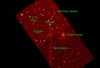 |
Fig. 1. Chandra image in the 0.3–5 keV energy band after a Gaussian smoothing. The positions of the pulsar, the nebulae, and the serendipitous Galaxy cluster are labeled. The image axes are aligned in right ascension and declination with north to the top and east to the left. The angle θ used for the MRHT is defined such that zero is at 90° toward east with respect to the north Celestial Meridian and is measured in the counter-clockwise direction from 0° to 180°. |
3. X-ray data analysis
3.1. Pulsar proper motion
We performed relative astrometry on our two-epoch Chandra images to search for the proper motion of the pulsar. We used the same approach adopted to study the proper motion of PSR J0357+3205 (De Luca et al. 2013). For each observation, we generated an image in the 0.3–8 keV energy range using the original ACIS pixel size ( ). We ran a source detection using the wavdetect task, with wavelet scales ranging from 1 to 16 pixels with a
  step, setting a detection threshold of 10−6. The resulting source catalogs were cross-correlated with a correlation radius of 3″ to extract the list of sources detected at both epochs. The chance alignment probability of two false detections is of order ∼10−5, based on the density of sources in the two images. We selected sources within 4′ of the aim point, since point source localization accuracy deteriorates beyond that distance because of degradation of the point spread function (PSF) with offset angle (see discussion in De Luca et al. 2009). We only used sources with a signal-to-noise larger than 4 (srcsignificance parameter in wavdetect source list). The resulting list includes 20 field sources and the pulsar counterpart. The positions of the 20 sources, which have uncertainties ranging from 0.04 pixel to 0.3 pixel per coordinate, were used as a reference grid for relative astrometry. We computed the best transformation to superimpose the reference frames of the two images collected at different epochs. After rejecting 3 sources yielding large residuals (at more than 3.5σ), a simple translation yielded a good result (see Fig. 2): an rms deviation of ∼0.3 pixel per coordinate on the reference sources and an uncertainty of ∼30 mas per coordinate on the frame registration. More complex geometric transformations are not statistically required. We then applied the optimized transformation to the coordinates of the pulsar counterpart to investigate its possible displacement between the two epochs. The overall uncertainty in the pulsar displacement includes the uncertainty in the pulsar localization in each image and the uncertainty in the image superposition. Our results are shown in Fig. 2. The pulsar counterpart shows a tiny displacement, roughly pointing in the counter-direction of the secondary nebula, but its statistical significance (≲2σ) is too low to allow any claim; indeed, such a displacement is comparable to the residuals in the positions of the reference stars after the frame registration. Thus, we assume the corresponding yearly angular displacement, together with errors at the 3σ level, as a conservative upper limit on the pulsar proper motion. We conclude that the upper limits on the proper motion of J2055 are μα cos(δ) < 125 mas yr−1 and μδ < 200 mas yr−1.
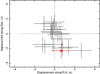 |
Fig. 2. Displacement of sources within 4′ of the Chandra aim point between the two epochs of Chandra observations. The displacement of the pulsar is shown by the red star. |
3.2. Small-scale analysis of the nebulae
Using the standard CIAO tools Marx and Chart, we simulated a point-like source at the same position on the detector and with the same spectrum as the J2055 pulsar but with an exposure time of 1 Ms (∼10 times our observation). Then, we produced circular brightness distributions of the simulated source and counts actually detected from the pulsar. The distributions for the pulsar and the simulated source are consistent, indicating no bright extended emission within 2″ of the pulsar. Using this method, we found that a possible bow shock located between  and 1″ from the pulsar would be detected at 3σ with more than ∼75 counts during our 96.8 ks long exposure (also considering the PSF of this source). Taking into account the interstellar absorption along the line of sight to the source and a power-law spectrum with Γ ∼ 2 from Marelli et al. (2016), this results in an upper limit of ∼1.5 × 10⁻¹⁴ erg cm−2 s−1 to the unabsorbed flux of a bow shock. Below
  the emission would not be disentangled from the point-like emission owing to the Chandra pixel dimension (
 ).
).
The previous method results in a poor description of the linear feature protruding from the pulsar, given that the brightness is evaluated over circular annuli. A linear brightness distribution, taken from boxes that are 10′ thick along the main axis of the brightest nebula, detects extended emission protruding directly from the pulsar; there is a decrease of a factor ∼2 in brightness within 20″ of the pulsar. Figure 3 shows the two distributions.
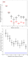 |
Fig. 3. Top panel: circular brightness distribution of the simulated source (red) and the background-subtracted pulsar (black). Within 2″, where the contribution of the main nebula is negligible, the two distributions are in agreement. Bottom panel: linear brightness distribution of the main nebula along its main axis (black) within 1′ of the pulsar. We also show the predicted background (blue line). We excluded a circular region of 2″ radius around the pulsar, where point-like emission dominates. |
3.3. Large-scale analysis of the nebulae
In order to determine the main axes of the nebulae, we ran a modified RHT for the main nebula and secondary nebula separately (see Appendix A.5 for details). We modeled both structures using different segment lengths ls. We analyzed the distribution of the angles, ignoring the position of the segments. For lengths comparable to the nebular length (∼8′ and  for the main and secondary Nebula, respectively), the distribution of segment angles θs is expected to have a peak at the angle of the main axis of the nebula. For smaller lengths, the distribution depends on the ls/ts ratio, where ts is the mean nebular thickness and nebular small-scale structure, as shown in Figs. 4 and 5. Using the CIAO tool mkpsfmap, we checked that the variation of the Chandra PSF in the field of view (FoV) cannot substantially affect this result.
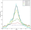 |
Fig. 4. Histogram of the angles obtained through the MRHT for a subsample of segment lengths for the main nebula analysis. Each segment is weighted using its H-value. The histogram integrals are normalized to one. We report the best fit of a constant plus Gaussian for the best segment using 80° < θ < 100°. |
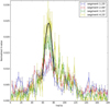 |
Fig. 5. Histogram of the angles obtained through the MRHT for a subsample of segment lengths for the secondary nebula analysis. Each segment is weighted using its H-value. The histogram integrals are normalized to one. We report the best constant plus Gaussian fit for the longest segment using 58° < θ < 82°. |
As expected, the highest value of the maximum point of the distribution of angles, Hmax, is reached using a segment length ls of ∼8′ and  for the main and secondary Nebula, respectively. Using this length, the nebula is best represented by a beam of segments with angles that peak around its main axis. On the basis of the behavior shown, we can evaluate the angle of the main axis of the nebula by fitting the peak of the distribution obtained for ls ∼ 8′ with a Gaussian plus a constant. The maximum of the Gaussian distribution and its error can be taken as a measure of the angle of the main axis of the main nebula of J2055. We obtain
  for the main axis of the main nebula and
  for the main axis of the secondary nebula. The angle between the two nebulae is
  . This is in agreement within 3σ with the result of
  from the XMM-Newton observation, obtained using an independent method (Marelli et al. 2016). The small difference between the two results can arise from the observation of the entire main nebula (12′) in XMM-Newton data, while we are considering only the first
  visible with Chandra. Since the line angle occurrences are not statistically independent because they are derived from overlapping fractions of the same image, the estimation of errors described above is not formally correct and the errors of the angle distribution histograms may be underestimated. We created 100 simulated data sets with a uniform, straight feature 15″ thick, 8′ long that has a brightness comparable to the faintest part of the real nebula (a total number of counts of 50% of the observed nebula); we also considered effects introduced by the Chandra PSF and exposure map. After running the MRHT on these 100 simulated images, we extracted the maximum angle, as before, and used these to evaluate the correct dispersion around the real value. The uncertainty estimates obtained through simulations were consistent (within 10%) with the results obtained from the Gaussian fits applied to the real data.
3.4. Analysis of the shape of the nebulae
Having determined the main axes of the nebulae, we can quantify their variation with both classical and MRHT modeling. The first method gives the event distribution around the axis while the second method gives the best modeling of the nebulae through linear segments. We extracted counts from boxes centered along the main axis of each nebula, each covering  . We normalized for the area such that the results are in counts arcsec−2, we applied an exposure correction, and accurately subtracted point-like sources and background. For each box, we produced histograms reporting the background-subtracted brightness perpendicular to the main axis with bins of
  . For each pair of adjacent boxes, we applied a Student’s t-test to the histograms to evaluate the consistency of the two distributions, and we also fitted each distribution with a Gaussian. In the case of adjacent distributions being consistent within 3σ (according to the t-test) and all parameters of the Gaussian fits also being consistent within 3σ, we merged the two contiguous boxes, obtaining a sort of adaptive binning. We iterated this process until the distribution in each box differs significantly from the adjacent boxes. Using such a division, we defined the thickness of the nebula in each box as the width of the rectangular region that comprises 95% of the nebular counts in the selected box. The effect of the Chandra PSF was taken into account by simulating PSF maps with the mkpfsmap CIAO tool and by applying the following correction:
  , where σPSF is derived from a Gaussian fit of the radial profile of a simulated point-like source. Because of the small PSF size with respect to the nebular observed thickness, the error on the Gaussian approximation of the PSF is negligible. The results are reported in Table 1 and the central panel of Fig. 6. The main nebula is thinner and brighter for the first 2′ from the pulsar; in this case, the nebula points toward the east. From 2′ to 6′ the nebula is wider, with a fluctuating brightness, reaching the maximum thickness between 5′ and 6′. Between 7′ and 8′ the nebula is again thin almost at the level of the part nearest to the pulsar (but fainter) and points toward west. The secondary nebula is fainter, so that we only find a significant difference among the first and last half, with the nearest part thicker and/or fainter.
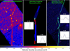 |
Fig. 6. Left panel: 0.3–5 keV Chandra image of the J2055 field. The image has been smoothed with a Gaussian filter. Central panel: graphical representation of the results of the imaging analysis presented in Sect. 3.4. Each box has a count distribution that varies significantly (3σ) from the adjacent distributions. The box thickness contains 95% of the background counts, as from Gaussian describing the distribution. The box intensity is the best-fitted (background-subtracted) counts density within the box. The pulsar position is indicated by a cyan X. We also report a sample of the distributions described in Table 1, where the distance orthogonal to the main axis of the nebula is on the x-axis and on the background-subtracted nebular counts is on the y-axis. Right panel: graphical representation of the results of the MRHT analysis presented in Sect. 3. Each cyan vector is the best-fitted maximum of a distribution significantly (3σ) different from the adjacent distributions. Dotted green lines show the 1σ error on the associated vector. The pulsar position is denoted by a cyan X. As for the central panel, we report a sample of the distributions described in Table 1, where the angle of significant segments from MRHT is on the y-axis. |
We followed a similar methodology using the results of the MRHT and distributions as defined in Sect. 3.3. In this case, the Gaussian fit is performed on angular instead of count distributions and only in the central part of the peak because of its complex shape. Again, we checked the errors on angles using simulations (100 realizations divided into 8 groups, 1 for each segment). The 1σ errors from the simulations are generally compatible with those from the Gaussian fit with a maximum increase of 30%. In Table 1 and Fig. 6 we report the results of the Gaussian fit. The MRHT results are compatible with the features coming from the previous method (see Table 1). For the main nebula, the angle is ∼100° for the first 2′ from the pulsar. From 2′ to 3′ it is heavily affected by the presence of the CCD gap. The main improvement from the MRHT comes from the variations seen between 3′ and 8′. Here, the nebula significantly fluctuates around the main axis on an arcminute scale, reaching a value of ∼80° in the last arcminute.
The secondary nebula is too faint to obtain any significant division. However, the MRHT approach models it with a single segment that passes through the pulsar position (within 1σ), thus confirming the association with the pulsar and a general symmetry around the main axis. The results of the two analyses are reported in Table 1 and the central and right panel of Fig. 6.
4. Optical observations and data analysis
To search for alternative evidence of the pulsar motion and determine its direction in the plane of the sky, we looked for an arc-like emission structure from ionized hydrogen produced at the termination shock of the pulsar wind as it moves supersonically in the interstellar medium (ISM). To detect such a bow shock, we obtained deep observations of the J2055 field with the GTC on August 22 and 23, 2015 under program GTC12-15A. We observed J2055 with the Optical System for Imaging and low Resolution Integrated Spectroscopy (OSIRIS). The instrument is equipped with a two-chip E2V CCD detectors with a nominal FoV of 7′ × 7′. The pixel size of the CCD is  in the 2 × 2 binning mode. We took three sequences of 15 exposures in the Hα filter (λ = 6530 Å; Δλ = 160 Å) with exposure time of 155 s each to minimize the saturation of bright stars in the field and remove cosmic ray hits. We also took one sequence of 15 exposures (also of 155 s each) in the r′ (λ = 6410 Å; Δλ = 1760 Å) filter. In order to cover as much of the main nebula as possible, the pointing coordinates were offset by 2′ to the east and 2′ to the south. Observations were performed in gray and clear sky conditions with an average airmass of 1.22 and a seeing of
  . Short (0.5–3 s) exposures of standard star fields (Smith et al. 2002) were also acquired for photometric calibration, together with twilight sky flat fields.
We reduced our data (bias subtraction, flat-field correction) using standard tools in the IRAF4 package CCDRED. Per each filter, single dithered exposures were then aligned, average-stacked, and filtered for cosmic rays using the IRAF task drizzle. We computed the astrometry calibration on the GTC images using the wcstools5, matching the sky coordinates of stars selected from the Two Micron All Sky Survey (2MASS) All-Sky Catalog of Point Sources (Skrutskie et al. 2006) with their pixel coordinates computed by Sextractor (Bertin & Arnouts 1996). After iterating the matching process applying a σ-clipping selection to filter out obvious mismatches, high-proper motion stars, and false detections, we ended up with an overall accuracy of ∼ on our absolute astrometry.
We did not detect any arc-like structure that could be identified as a bow shock associated with the pulsar in the stacked Hα image. We computed a 3σ surface brightness limit on the undetected bow shock from the rms of the sky background sampled within a radius of 5″ of the pulsar position, conservatively set to account for the uncertainty on the stand-off distance between the pulsar and the bow-shock apex (see Sect. 5). We note that the pulsar falls ∼2″ southwest from a star (r′ = 20.34 ± 0.04; Mignani et al. 2018), which increases the rms of the sky background near to it. However, this would not dramatically affect our limit unless the bow-shock axis and the pulsar proper motion direction were pointing at the star at a position angle of ∼55° (incompatible with that of the main and secondary nebulae), its stand-off distance were of the same order of the pulsar/star separation, and its angular size were smaller than the image PSF. We converted instrumental magnitudes to physical flux units by cross-calibrating the Hα image against the r′ band image. To this aim, we matched about 500 stars in common between the two images (1″ matching radius) detected by Sextractor at 5σ above the background, after filtering saturated stars, blends, and stars too close to the CCD edges. We compared the instrumental magnitudes of the stars through aperture photometry using an aperture of  diameter, i.e., about three times the average seeing. We applied a linear fit between the instrumental magnitudes to obtain the relative photometry transformation after applying a σ clipping to filter out mismatches and outliers. This turned out to be accurate to within ±0.2 mag. By applying the r′ band night zero points and the airmass correction using the atmospheric extinction coefficients for the La Palma Observatory6 we then obtained a 3σ surface brightness limit of ∼2.3 × 10⁻¹⁷ erg cm−2 s−1 arcsec−2 in the Hα filter, which we assume as the upper limit on the surface brightness of the bow shock within a 5″ distance from the pulsar.
5. Discussion
We analyzed two new Chandra data sets of the J2055 system, focusing our analysis on the small- and large-scale shape of the nebular features protruding from the pulsar and on the search for the pulsar proper motion. We based the imaging analysis on the combination of a classical method and a newly developed method for the analysis of linear features called the modified rolling Hough transformation (MRHT).
We do not find evidence of proper motion down to 240 mas yr−1 (3σ level), which translates into an upper limit on the transverse velocity of ∼700 km s−1 at 600 pc. If we consider the system to be 600 pc distant, the angular lengths of 12′ for the main nebula and 250″ for the secondary nebula (Marelli et al. 2016) translate into projected physical lengths of 2.1 and 0.7 pc, respectively. Both values are consistent with other observed X-ray synchrotron nebulae, which show projected lengths up to a few parsecs (see, e.g., Kargaltsev et al. 2008, 2017). Considering our upper limit on the transverse velocity, the pulsar covered the lengths of the nebulae in tp > 3 kyr or tp > 1 kyr, respectively. Taking into account the classical sychrotron-emitting nebula model, the electrons are accelerated at the termination shock and injected into the cavity produced by the fast-moving pulsar. As discussed in Marelli et al. (2016), using optimistic values of ambient magnetic field and Lorentz factor for electron acceleration we obtain a synchrotron cooling time of the emitting electrons of τsync ∼ 100 yr ≪ tp. In order to reach the physical extension of the nebula, we thus need a bulk flow speed of the emitting particles >20 000 km s−1 and >7000 km s−1, respectively, for the two nebulae. The first value is only marginally consistent with results in the literature, while the second is fully consistent (Kargaltsev et al. 2008). Also, the lack of spectral variation in the main nebula (Marelli et al. 2016) points to a much higher bulk flow velocity or a reacceleration mechanism along this nebula. Thus, the classical synchrotron nebula model is disfavored in explaining the main nebula emission.
For classical synchrotron nebulae, we expect a relatively bright diffuse emission surrounding the pulsar, where the emission from the wind termination shock is brightest, as observed in all the other known cases (e.g., Kargaltsev & Pavlov 2008). Although there is not a clear correlation, typical luminosities of the “bullet” component versus the “tail” component are Lbull/Ltail > 0.1. Assuming the standard relations from Gaensler & Slane (2006), the distance between the pulsar and the head of the termination shock is expected to be  , where ρISM is the ambient density and νPSR is the pulsar velocity. Taking into account a typical ambient density (0.1 atoms cm−3) and our upper-limit velocity at 600 pc, this would place the shock at
  or further in case of a lower pulsar velocity. On a sub-arcsec angular scale, we do not find any evidence of a termination shock at ≳
 with an unabsorbed flux >1.5 × 10⁻¹⁴ erg cm−2 s−1. This makes the bullet component of the nebula fainter than expected if the main nebula is a typical synchrotron nebula, with Lbull/Ltail < 0.05. As reported in Marelli et al. (2016) the low energetics of the powering pulsar (Ė = 5.0 × 1033 erg s−1) also disfavor the model of a classical synchrotron-emitting nebula for the bright main feature. The luminosity of the secondary, fainter nebula instead is compatible with a classical PWN, both regarding the luminosity ratio Lbull/Ltail < 0.25 as well as the comparison of the nebula luminosity with the pulsar energetics.
The deep upper limits on the surface brightness of any undetected diffuse structure in our Hα images, coupled to the upper limit on the proper motion of the pulsar, allow us to constrain the properties of the ISM in the region surrounding the pulsar. Assuming the distance to the pulsar to be smaller than 900 pc, and the pulsar space velocity vector to point within 25° of the plane of the sky, the scaling relations proposed by Cordes et al. (1993) and Chatterjee & Cordes (2002; see also Pellizzoni et al. 2002) imply a neutral hydrogen fraction lower than 0.2, suggesting that the pulsar should be moving in the warm or hot component of the ISM. Some contribution to the ionization of the ISM could of course be due to the UV flux from the pulsar itself.
Through the MRHT approach we determined the main axes of the two features, separated by  . The evaluation of the main axes of the two nebular structures also allowed us to produce results from classical methods. The main nebula is tight and has a 95% thickness 9″ < t95 < 31″ because this feature is thinner nearby and far from the pulsar; this feature is evaluated on an arcminute-scale along the first
  of the observable nebula (out of the 12′ seen by XMM-Newton) and also directly protrudes from the pulsar on an arcsecond scale. The brightness profile changes with distance on an arcmin scale because it is wider for distance 2′< d < 7′ and brighter near the pulsar (d < 1′) and far from it (7′ < d < 8′). On a similar scale, the direction of the nebula also changes in the range 71° < θ < 92° for 3′ < d < 8′, where the angle θ is defined such that the zero is at 90° due east with respect to the north Celestial Meridian and is measured in the counter-clockwise direction; this nebula follows a snake-like shape.
Normal to the main axis, the distributions of the nebular counts are not uniform with distance from the pulsar. Moreover, both the classical analysis and the MRHT detect hints of a split in the structure of the wider segments, 5′ < dpulsar < 6′ and 6′< dpulsar < 7′. For the classical method, this comes from the wider peak in the distribution between 5′ < dpulsar < 6′ (see Table 1 and panel in Fig. 6), which is not supported by a similar widening in the angles and thus points to parallel structures. For the MRHT method, this is also apparent in Fig. A.3, left panel, when we use a segment length of 1′. This resembles a single (or multiple, if the split is confirmed) helicoidal pattern, although we cannot exclude an irregular short-scale-bumped shape. Given the fainter and less collimated nature of the secondary nebula, compared to the main nebular, apart from its direction, we can only infer a hint of narrowing with distance and a roughly symmetric profile perpendicularly to its main axis. Only future deeper Chandra observations will be able to better define the nebular structures.
We found four other pulsars in the literature associated with elongated parsec-long features misaligned with the proper motion direction. The pulsar PSR B2224+65 (Hui & Becker 2007) is associated with a long, extended X-ray feature whose orientation deviates by ∼118° from a classical bow-shock nebula (the Guitar Nebula), seen in Hα in the counter-direction of the proper motion. An X-ray counter-feature of the X-ray nebula was also detected (Johnson & Wang 2010), albeit substantially fainter and shorter than the main nebular. PSR J1101−6101 (Halpern et al. 2014) is associated with the long, collimated Lighthouse Nebula, which deviates by ∼104° from a classical X-ray PWN in the counter-direction of the presumed proper motion direction (Pavan et al. 2014). This nebula is well modeled by a (multi)helical pattern. A short, faint counter-feature of the Lighthouse Nebula is also detected in X-rays. This system also comprises a classical PWN, counter-aligned with the pulsar proper motion direction and less collimated than the other two structures. PSR J1509−5850 is associated with a parsec-long X-ray PWN (Kargaltsev et al. 2008) extending in the counter-direction of the proper motion. Recently, a fainter elongated, parsec-long feature has been detected in X-rays, deviating by ∼147° from the brighter nebula (Klingler et al. 2016a). Finally, PSR B0355+54 is associated with the Mushroom X-ray PWN, oriented in the counter-direction of the proper motion. Hints of two faint, short, counter-aligned features have been observed in X-rays, one of which is twice the length of the other, almost orthogonal to the pulsar proper motion direction (Klingler et al. 2016b).
Taking into account the rotational energy loss that is converted into the luminosities of the misaligned features, we obtain values 0.0004 < Lbol/Ė < 0.07 (with a value of 0.0064 for J2055) and typical projected lengths 0.7 < lproj < 7.7 pc (with a value of ∼2.1 pc at 600 pc for J2055), while the energetics of the powering pulsars span three orders of magnitude (from ∼1033 to ∼1036 erg s−1). For a general view of such nebulae see Fig. 9 in Kargaltsev et al. (2017).
In the case of J2055, the possible helical morphology of the main nebula resembles the Lighthouse Nebula, among the four cited cases. The secondary nebula can hardly be interpreted as a counter-feature of the main nebular, given the misalignment of the two features, in particular taking into account only the first part of the main nebula. Also, all the other known counter-features are collimated, and the secondary nebula is not. It is more consistent, given the energetics, direction, and low collimation, with a classical PWN as in the case of the classical PWN of the Lighthouse system.
To explain the nature of the motion-misaligned, collimated features such as the main nebula of J2055, two models are commonly invoked. Bandiera (2008) considered a scenario in which high-energy particles leak from the termination shock apex into the ISM and travel along the ordered ISM magnetic field. The main problem with this scenario is the lack (or faintness) of counter-features, which means that there is a preferred direction for the escape of particles. The cause of such an asymmetry is unclear. Although a Doppler effect could be invoked, the discussion is still open (see, e.g., Klingler et al. 2016a; Kargaltsev et al. 2017). As reported in Pavan et al. (2014), the helical pattern of the J2055 nebula weakens an interpretation based on this model. The second model invokes a powerful, collimated ballistic jet from the pulsar poles. Such jets should be bent by the ram pressure of the oncoming ISM, while the lack (or faintness) of the counter-feature is explained in terms of Doppler boosting. Such an interpretation is particularly intriguing for the Lighthouse Nebula, whose shape is well modeled by a (single or multiple) helical pattern. This is ascribed to the precession of the pulsar (possibly due to its oblateness) or kink instabilities in the jet. A comprehensive discussion of this model is given in Pavan et al. (2014, 2016). The shape of the J2055 main nebula is reminiscent of the Lighthouse Nebula, only coming from a pulsar that is ∼200 times less energetic and ∼10 times nearer.
For both nebular models, a key role could be played by the geometry and magnetic field configuration of the powering pulsar. Unlike PSR J1101−6101, J2055 is a strong emitter of γ-ray radiation and models have been developed to describe its magnetic field configuration. The second Fermi pulsar catalog (Abdo et al. 2013) reports that J2055 is one of the very few γ-ray pulsars with a strong detection of off-pulse emission characterized by a spectral cutoff: this emission probably originates from its magnetosphere, opening a new conundrum for magnetospheric emission models. Such weakly pulsed emission should be rare as it is expected only for nearly aligned pulsators seen at high inclinations using classic outer-gap models (Romani & Watters 2010). Pierbattista et al. (2015) used different γ-ray and radio emission geometries to fit γ-ray and radio light curves of Fermi pulsars, where outer-gap and one-pole caustic emission models are favored in explaining the pulsar emission pattern of Fermi pulsars. Among these, J2055 is best fitted using models where γ-ray emission comes from near the pulsar surface, such as the Polar Cap (Muslimov & Harding 2003) and Slot Gap (Muslimov & Harding 2004) models, while outer-magnetosphere models fail to predict the light curve shape correctly. We note that such models are usually disfavored in describing pulsar emission (see, e.g., Abdo et al. 2013; Pierbattista et al. 2015); there are some notable exceptions (see, e.g., PSR J0659+1414; Weltevrede et al. 2010) and J2055 could well be one of these few exceptions.
This suggests that J2055 could have a rare geometry, although the exact nature of that shap is still unclear. This geometry could be the key to understanding why only a small number of pulsars show such powerful, collimated features, and how they are produced.
More observations, as well as the application of new analysis techniques and models, could help us to understand the shape and spectrum of such misaligned nebulae. Deep investigations of pulsars with geometrical configurations similar to J2055 would also greatly help to develop models for such features, clarifying the role of the magnetic field of the pulsar in the creation of such powerful, extended sources.
6. Conclusions
Using two recently obtained Chandra observations of PSR J2055+2539, we set an upper limit on its proper motion of 240 mas yr−1, which translates into an upper limit on its transverse velocity of ∼700 km s−1 at 600 pc. We found no evidence of bow shocks, either in the X-rays or in Hα, at scales ≳ . Two almost-linear features protrude from the pulsar. The main, brighter nebula is highly collimated and its shape is reminiscent of a (multi)helicoidal pattern, resembling the long, motion-misaligned feature seen in the Lighthouse Nebula. Because of its brightness, shape, lack of a bow shock, and low pulsar energetics we rule out the main nebula as a classical PWN. Four other known systems present long, very collimated nebulae misaligned with the pulsar proper motion, one of which has a (multi)helicoidal shape. We conclude that the main nebula is produced by the same physical process as these four. We speculate that this process might be related to a peculiar geometry of the magnetosphere of the powering pulsar, which is confirmed in the case of J2055 via its γ-ray properties.
The secondary nebula is consistent with a classical PWN model, based on the pulsar energetics and nebular luminosity, and on the lack of a detected bow shock. However, only future observations including the detection of the pulsar proper motion can confirm our hypothesis.
IRAF is distributed by the National Optical Astronomy Observatories, which are operated by the Association of Universities for Research in Astronomy, Inc., under cooperative agreement with the National Science Foundation.
Acknowledgments
We thank Nanda Rea for the use of the data of GTC under program GTC12-15A and for the useful discussion. We thank the referee for the useful comments that really improved the paper in many ways. This work was supported by the Fermi contract ASI-INAF I-005-12-0. This work was supported by the IUSS contract for the project “Studio del cielo ad alte energie: variabilitá del cielo nei raggi X oltre EXTraS e nei raggi gamma in vista del CTA”. RPM acknowledges financial support from an INAF “Occhialini Fellowship”. Support for this work was provided by the National Aeronautics and Space Administration through Chandra Award Number GO5-16076X issued by the Chandra X-ray Center, which is operated by the Smithsonian Astrophysical Observatory for and on behalf of the National Aeronautics Space Administration under contract NAS8-03060.
References
- Abdo, A. A., Ackermann, M., Ajello, M., et al. 2009, ApJS, 183, 46 [NASA ADS] [CrossRef] [Google Scholar]
- Abdo, A. A., Ajello, M., Allafort, A., et al. 2013, ApJS, 208, 17 [NASA ADS] [CrossRef] [Google Scholar]
- Ackermann, M., Ajello, M., Baldini, L., et al. 2011, ApJ, 726, 35 [NASA ADS] [CrossRef] [Google Scholar]
- Aschwanden, M. J. 2010, SoPh, 262, 235 [Google Scholar]
- Bertin, E., & Arnouts, S. 1996, A&AS, 117, 393 [NASA ADS] [CrossRef] [EDP Sciences] [Google Scholar]
- Bandiera, R. 2008, A&A, 490, 3 [Google Scholar]
- Chatterjee, S., & Cordes, J. M. 2002, ApJ, 575, 407 [NASA ADS] [CrossRef] [Google Scholar]
- Clark, S. E., Peek, J. E. G., & Putman, M. E. 2014, ApJ, 789, 82 [NASA ADS] [CrossRef] [Google Scholar]
- Cordes, J. M., Romani, R. W., & Lundgren, S. C. 1993, Nature, 362, 133 [NASA ADS] [CrossRef] [Google Scholar]
- De Luca, A., Caraveo, P. A., Esposito, P., et al. 2009, ApJ, 692, 158 [NASA ADS] [CrossRef] [Google Scholar]
- De Luca, A., Mignani, R. P., Marelli, M., et al. 2013, ApJ, 765, L19 [NASA ADS] [CrossRef] [Google Scholar]
- Gaensler, B. M., & Slane, P. O. 2006, ARA&A, 44, 17 [NASA ADS] [CrossRef] [Google Scholar]
- Gaensler, B. M., van der Swaluw, E., Camilo, F., et al. 2004, ApJ, 616, 383 [NASA ADS] [CrossRef] [Google Scholar]
- Garmire, G. G., Bautz, M. W., Ford, P. G., et al. 2003, SPIE, 4851, 28 [Google Scholar]
- Duda, R. O., & Hart, P. E. 1972, Comm. ACM, 15, 11 [CrossRef] [Google Scholar]
- Halpern, J. P., Tomsick, J. A., Gotthelf, E. V., et al. 2014, ApJ, 795, 27 [NASA ADS] [CrossRef] [Google Scholar]
- Hui, C. Y., & Becker, W. 2007, A&A, 467, 1209 [NASA ADS] [CrossRef] [EDP Sciences] [Google Scholar]
- Illingworth, J., & Kittler, J. 1988, Graphics Image Process., 44, 1 [CrossRef] [Google Scholar]
- Jelic, V., Prelogovic, D., Haverkorn, M., Remeijn, J., & Klindzic, D. 2018, A&A, 615, L3 [NASA ADS] [CrossRef] [EDP Sciences] [Google Scholar]
- Johnson, S. P., & Wang, Q. D. 2010, MNRAS, 408, 1216 [NASA ADS] [CrossRef] [Google Scholar]
- Kargaltsev, O., & Pavlov, G. G. 2008, in 40 Years of Pulsars: Millisecond Pulsars, Magnetars and More, eds. C. G. Bassa, Z. Wang, A. Cumming, & V. M. Kaspi (Melville, NY: AIP), AIP Conf. Proc., 983, 171 [Google Scholar]
- Kargaltsev, O., Misanovic, Z., Pavlov, G. G., Wong, J. A., & Garmire, G. P. 2008, ApJ, 684, 542 [NASA ADS] [CrossRef] [Google Scholar]
- Kargaltsev, O., Pavlov, G. G., Klingler, N., & Rangelov, B. 2017, J. Plasma Phys., 83, 5 [Google Scholar]
- Klingler, N., Kargaltsev, O., Rangelov, B., et al. 2016a, ApJ, 828, 70 [NASA ADS] [CrossRef] [Google Scholar]
- Klingler, N., Rangelov, B., Kargaltsev, O., et al. 2016b, ApJ, 833, 253 [NASA ADS] [CrossRef] [Google Scholar]
- Marelli, M., De Luca, A., Salvetti, D., et al. 2013, ApJ, 765, 36 [NASA ADS] [CrossRef] [Google Scholar]
- Marelli, M., Belfiore, A., Saz Parkinson, P., et al. 2014, ApJ, 790, 51 [NASA ADS] [CrossRef] [Google Scholar]
- Marelli, M., Pizzocaro, D., De Luca, A., et al. 2016, ApJ, 819, 40 [NASA ADS] [CrossRef] [Google Scholar]
- McGowan, K. E., Vestrand, W. T., Kennea, J. A., et al. 2006, ApJ, 647, 1300 [NASA ADS] [CrossRef] [Google Scholar]
- Mignani, R. P., Testa, V., Rea, N., et al. 2018, MNRAS, 478, 332 [NASA ADS] [CrossRef] [Google Scholar]
- Muslimov, A. G., & Harding, A. K. 2003, ApJ, 588, 430 [NASA ADS] [CrossRef] [Google Scholar]
- Muslimov, A. G., & Harding, A. K. 2004, ApJ, 606, 1143 [NASA ADS] [CrossRef] [Google Scholar]
- Pavan, L., Bordas, P., Puhlhofer, G., et al. 2014, A&A, 562, A122 [NASA ADS] [CrossRef] [EDP Sciences] [Google Scholar]
- Pavan, L., Puhlhofer, G., Bordas, P., et al. 2016, A&A, 591, A91 [NASA ADS] [CrossRef] [EDP Sciences] [Google Scholar]
- Pellizzoni, A., Mereghetti, S., & De Luca, A. 2002, A&A, 393, 65 [NASA ADS] [CrossRef] [EDP Sciences] [Google Scholar]
- Pierbattista, M., Harding, A. K., Grenier, I. A., et al. 2015, A&A, 575, A3 [NASA ADS] [CrossRef] [EDP Sciences] [Google Scholar]
- Posselt, B., Pavlov, G. G., Slane, P. O., et al. 2017, ApJ, 835, 66 [NASA ADS] [CrossRef] [Google Scholar]
- Romani, R. W., & Watters, K. P. 2010, ApJ, 714, 810 [NASA ADS] [CrossRef] [Google Scholar]
- Saz Parkinson, P. M., Dormody, M., Ziegler, M., et al. 2010, ApJ, 725, 571 [NASA ADS] [CrossRef] [Google Scholar]
- Skrutskie, M. F., Cutri, R. M., Stiening, R., et al. 2006, AJ, 131, 1163 [NASA ADS] [CrossRef] [Google Scholar]
- Smith, J. A., Tucker, D. L., Kent, S., et al. 2002, AJ, 123, 2121 [Google Scholar]
- Temim, T., & Slane, P. 2017, ASSL, 446, 29 [NASA ADS] [Google Scholar]
- Weltevrede, P., Abdo, A. A., Ackermann, M., et al. 2010, ApJ, 708, 1426 [NASA ADS] [CrossRef] [Google Scholar]
Appendix A: Modified rolling Hough transformation with application to Chandra data
The Hough transformation (HT) was first used for the detection of complex patterns in bubble chamber photographs (Duda & Hart 1972). Soon, it proved to be a powerful tool for the detection of linear patterns and has found many applications in image processing (Illingworth & Kittler 1988). Clark et al. (2014) adapted the HT in a rolling version (RHT) to study linear HI features in the diffuse Galactic ISM. This method was recently used also by Jelic et al. (2018). We adapted the RHT for a global characterization of X-ray observations, which usually have lower statistics than optical observations. Through the comparison of the input image with an expected, simulated background image, we are able to extract the significance of each segment in the pattern. In order to apply our MRHT algorithm, we also need to flatten the Chandra background through the careful handling of contaminating celestial sources, exposure-map variation, and different chip illumination. The MRHT approach and the flattening of Chandra background applied to our observation are described in Appendix A.4. As a final step, the MRHT produces a list of segments with a significance Ss > 3.5σ characterized by the following six parameters:
-
ls, the length of the segment (that is given as input);
-
(xs, ys), the position of the center of the segment;
-
θs, the angle of the segment, from 0° to 180°, defined such that the zero is at 90° due east with respect to the north Celestial Meridian and measured in the counter-clockwise direction (see Fig. 1);
-
Ss, the significance of the segment in units of standard deviations;
-
Hs, the density of exposure-corrected events falling on the segment in counts/pixel units.
A.1. Hough transformation
Our implementation of the Hough transformation follows that of Duda & Hart (1972). In this basic implementation, given a Cartesian coordinate space (x−y), a straight line in this space can be described through the angle θ of its normal passing through the origin and the minimum Euclidean distance ρ from the origin, as follows:
 (A.1)
(A.1)
Each single (xi, yi) event pixel in the image (x−y) space can be, therefore, transformed into a sinusoidal curve in the ρ−θ parameter space, where ρ = xi cosθ + yi sinθ. The sinusoid beams that result from transformed colinear points in the image space have a common point of intersection (ρ0, θ0) in the parameter space. The parameters (ρ0, θ0) describe the line that passes through such colinear points in the image space. Usually the ρ−θ space is quantized to reduce the computational burden considerably. The Hough transformation thus stores in a (ρ, θ) array the number of events in the image space that contribute to each pixel in the parameter space H(ρ, θ), basically, the number of events for each line in the image space. Thus, the problem of detecting colinear points in the image space can be converted to the problem of finding bright pixels in the parameter space. Setting an intensity threshold Hthresh in the parameter space, the most prominent lines in the image space can be extracted and represented in the image space. The obvious limitations of this method are
-
it can only be used to detect straight, bright lines that significantly contribute to the entire image space;
-
it cannot assign to each line the probability of being spurious, only allowing for a user-selected intensity cut; and
-
it is not sensitive to background spatial variations.
A.2. Rolling Hough transformation
The rolling Hough transformation performs a Hough transformation N times on circular sub-images, extracted from a circular region with a given diameter D and center (xc, yc). For each sub-image the parameter space is limited to ρ = 0, so that the ρ−θ space is reduced to a one-dimensional space on θ, for each sub-image defined by (xc, yc). Only pixels in each (θ) sub-space (extracted from D-length segments centered in (xc, yc) in the image space) with intensity H(θ, xc, yc) over a user-set intensity threshold Hthresh are considered. A visualization of the linear structures identified by the RHT, the back-projection H(x, y) is obtained by integrating H(θ, xc, yc) over θ. The RHT approach has two main limits, when applied to the X-ray observations: First, to extract lines, the user must choose a given intensity, or intensity percentage that is not based on a statistical analysis. Second, this method requires a good statistics (e.g., in a Gaussian approach) for each circle analyzed with the Hough transformation, thus requiring sufficiently large circular regions in the sky.
A.3. Modified rolling Hough transformation
Following the same sub-selection of D-diameter circular images approach as in the RHT, we evaluate the threshold based on the probability PH that the line in the image space is spurious, rather than on a given intensity threshold Hthresh. This is possible thanks to Monte Carlo simulations run on a “flat background” image. We apply the RHT transformation on the simulated images to extract the mean histogram f(H) of H-values in the case of a source-free background. We can thus link the H-value(θ, xc, yc), basically the number of events on the segment in the image space defined by (θ, xc, yc), with the probability of being spurious, defined as
 (A.2)
(A.2)
It is straightforward to convert P(H) into a significance S(H) (expressed in σ). Lines in the image space below a probability threshold PH are discarded, while the others are stored and contribute to the back projection. This method is applied several times for a grid of extraction diameters D, thus allowing for the detection and characterization of segments of different lengths. A normalization that takes into account the segment length is applied (using H/D instead of H).
We note that this method requires a background that is as flat as possible. The probability is evaluated globally, thus a background spatial variation would result in a spatially variable sensitivity to features and, therefore, spurious detection of background features. Part of our work involved correcting instrumental features of the Chandra images, such as exposure map variations and different characteristics of individual CCDs, and the removal of contaminants such as point-like sources.
A.4. Flattening the Chandra background
In order to apply our modified RHT algorithm, we need to decrease the spatial variations of the Chandra background in our observations. There are four main sources of contamination as follows:
-
Celestial sources: Both the point-like sources and the detected Galaxy cluster (Marelli et al. 2016) could affect the characterization of the nebulae.
-
Exposure map: Variations in the exposure map result in a variation of the background count rate, affecting the global H-values distribution and resulting in a decrease of the HT sensitivity and detection of spurious, background-related lines.
-
Chip illumination: We perform our analysis on S2 and S3 Chandra CCDs, front-illuminated and back-illuminated, respectively; this results in a different background count rate level, and thus leads to the same problems coming from exposure map variations.
-
Unexposed areas: The presence of unexposed areas heavily affects the global H-values distribution and could hamper the analysis using long segments.
For the HT we worked on the 0.3–5 keV images and exposure maps. We cheesed them, excluding elliptical regions around each source containing 99% of expected source counts, as extracted by wavdetect. We also excluded the galaxy cluster in the S2 CCD using an ad hoc circular region, evaluated using both Chandra and XMM-Newton data.
We converted the standard exposure maps into fractional exposure maps, with each pixel (x, y) value Efrac defined as
 (A.3)
(A.3)
Vignetting effects within single chips are taken into account using vignetted exposures. Pixels with very low (<0.3) fractional exposure (3.1 and 2.6 arcmin2 on a total of 74.6 and 74.6 arcmin2 for CCD S2 and S3, respectively) were set to zero: for very low statistics the exposure correction diverges. Therefore these regions are excluded both from fractional exposure maps and images. To correct for exposure map variations, image pixel values are multiplied by the corresponding pixels values in the percentage exposure map.
We selected ad hoc source-free regions with high (>0.9), uniform exposure (22.3 and 50.9 arcmin2 for CCD S2 and S3, respectively). We extracted the (exposure-corrected) background count distribution from these regions. This distribution, after an area correction, was used to evaluate the probability of adding a new count in each pixel of cheesed area (where the exposure map of the CCD is not null).
Then, we co-added the two CCDs image maps, correcting for the different chip illumination. The two background distributions extracted from the two chips are compared using a Gaussian fit. We randomly added counts to the pixels of CCD 2 (front-illuminated, with the lower background) to correct for the different distributions.
As a final step, we added simulated counts to the unexposed areas following the distribution of the background of CCD 3 (Fig. A.1). This distribution is also used to create the simulated background image that we exploited for statistical analysis in our MRHT.
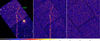 |
Fig. A.1. Results of our image reduction. Left panel: initial Chandra image. Central panel: we applied the analysis reported in Sect. A.4 to exclude field sources and flatten the Chandra background. In order to compare it with the simulated background, unexposed parts are filled as reported in Sect. A.4. Right panel: simulated Chandra background used to evaluate the significance of segments found through the MRHT (see Fig. A.2). |
A.5. Application of the MRHT to our Chandra data
In order to take into account the Chandra PSF, we re-binned the real and simulated images to have pixels of  . We run our modified RHT on these 0.3–5 keV, exposure-corrected, binned images (real image and background-simulated image).
For each pixel (xi, yi) within a circle centered at  and of 14′ diameter, our tool ran the HT in sub-circles of a given diameter and centered in (xi, yi). We ran our tool on simulated images for circles with diameters DW of 10, 20, 40, 60, 80, 100, 120, 140, 160, 180, 200, 240, 280, 320, 360, 400, 500, 600, and 700 pixels (from 15″ to 17′). The simulation of the image was repeated 1000 times, and the results were averaged. We made a quantization on the possible values of θ (from 0 to π) for each DW following the canonical (Clark et al. 2014)
 (A.4)
(A.4)
We thus extracted the histogram of H-values of the simulated background for each Dw (see Fig. A.2). In Fig. A.2 we also report the histogram of H-values obtained for the real image background, which is consistent with the simulated one. For each H0-value we can evaluate in the simulation the number of spurious detections above H0 renormalized over the entire number of detections. This represents the chance probability of a spurious detection P(H) in case of a homogeneous background, which can be used in the real image. Although the distribution is only quasi-Gaussian, as a first approximation we use the corresponding Gaussian σ instead of the probability.
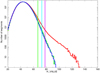 |
Fig. A.2. Distribution of H-values for Dw = 40 pixels (∼1′). The red histogram represents the distribution of the real image. The green histogram represents the distribution of the real background, clearly overlapping with the blue histogram, obtained from the simulated background, as expected. We highlight three different H-values with vertical lines, from left to right: 3σ (green), 3.5σ (cyan), and 4σ (violet), representing the chance probability of a spurious detection, as obtained from the simulations. The tail in the real image is apparent. |
As the final step, we ran the modified RTH on the real image, using the same prescriptions as before. We selected all the segments with an H-value corresponding to a chance probability >3.5σ, listing xc, yc, θ, Dw, S(H),Hval. This allows for a post-selection and analysis of high-significance segments or with a given length. We also obtain the back-projection image for each diameter and the total diameter (see Fig. A.3).
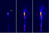 |
Fig. A.3. MHRT back-projection images for different Dw (∼1′, |


In order to analyze the two nebular features separately, we ran the modified RHT for the main nebula and secondary nebula separately. Thus, for each of these runs, the region containing the excluded feature is cheesed and replaced using the expected background distribution, as in the case of point-like sources and galaxy cluster. Finally, we also ran the script excluding both features to have the analysis of the background distribution. This revealed some slightly preferred angles due to unresolved point sources and residuals from the exposure map and instrumental corrections: this is therefore treated as a background for the MRHT results for the nebulae, where possible. Moreover, we only considered the segments with centers around the position of each of the two nebulae: a box of 150″ × 560″ for the main nebula and 75″ × 280″ for the secondary nebula. The regions extend starting from the pulsar, following the main angles of the nebulae.
All Tables
All Figures
|
Fig. 1. Chandra image in the 0.3–5 keV energy band after a Gaussian smoothing. The positions of the pulsar, the nebulae, and the serendipitous Galaxy cluster are labeled. The image axes are aligned in right ascension and declination with north to the top and east to the left. The angle θ used for the MRHT is defined such that zero is at 90° toward east with respect to the north Celestial Meridian and is measured in the counter-clockwise direction from 0° to 180°. |
| In the text | |
|
Fig. 2. Displacement of sources within 4′ of the Chandra aim point between the two epochs of Chandra observations. The displacement of the pulsar is shown by the red star. |
| In the text | |
|
Fig. 3. Top panel: circular brightness distribution of the simulated source (red) and the background-subtracted pulsar (black). Within 2″, where the contribution of the main nebula is negligible, the two distributions are in agreement. Bottom panel: linear brightness distribution of the main nebula along its main axis (black) within 1′ of the pulsar. We also show the predicted background (blue line). We excluded a circular region of 2″ radius around the pulsar, where point-like emission dominates. |
| In the text | |
|
Fig. 4. Histogram of the angles obtained through the MRHT for a subsample of segment lengths for the main nebula analysis. Each segment is weighted using its H-value. The histogram integrals are normalized to one. We report the best fit of a constant plus Gaussian for the best segment using 80° < θ < 100°. |
| In the text | |
|
Fig. 5. Histogram of the angles obtained through the MRHT for a subsample of segment lengths for the secondary nebula analysis. Each segment is weighted using its H-value. The histogram integrals are normalized to one. We report the best constant plus Gaussian fit for the longest segment using 58° < θ < 82°. |
| In the text | |
|
Fig. 6. Left panel: 0.3–5 keV Chandra image of the J2055 field. The image has been smoothed with a Gaussian filter. Central panel: graphical representation of the results of the imaging analysis presented in Sect. 3.4. Each box has a count distribution that varies significantly (3σ) from the adjacent distributions. The box thickness contains 95% of the background counts, as from Gaussian describing the distribution. The box intensity is the best-fitted (background-subtracted) counts density within the box. The pulsar position is indicated by a cyan X. We also report a sample of the distributions described in Table 1, where the distance orthogonal to the main axis of the nebula is on the x-axis and on the background-subtracted nebular counts is on the y-axis. Right panel: graphical representation of the results of the MRHT analysis presented in Sect. 3. Each cyan vector is the best-fitted maximum of a distribution significantly (3σ) different from the adjacent distributions. Dotted green lines show the 1σ error on the associated vector. The pulsar position is denoted by a cyan X. As for the central panel, we report a sample of the distributions described in Table 1, where the angle of significant segments from MRHT is on the y-axis. |
| In the text | |
|
Fig. A.1. Results of our image reduction. Left panel: initial Chandra image. Central panel: we applied the analysis reported in Sect. A.4 to exclude field sources and flatten the Chandra background. In order to compare it with the simulated background, unexposed parts are filled as reported in Sect. A.4. Right panel: simulated Chandra background used to evaluate the significance of segments found through the MRHT (see Fig. A.2). |
| In the text | |
|
Fig. A.2. Distribution of H-values for Dw = 40 pixels (∼1′). The red histogram represents the distribution of the real image. The green histogram represents the distribution of the real background, clearly overlapping with the blue histogram, obtained from the simulated background, as expected. We highlight three different H-values with vertical lines, from left to right: 3σ (green), 3.5σ (cyan), and 4σ (violet), representing the chance probability of a spurious detection, as obtained from the simulations. The tail in the real image is apparent. |
| In the text | |
|
Fig. A.3. MHRT back-projection images for different Dw (∼1′, |
| In the text | |
Current usage metrics show cumulative count of Article Views (full-text article views including HTML views, PDF and ePub downloads, according to the available data) and Abstracts Views on Vision4Press platform.
Data correspond to usage on the plateform after 2015. The current usage metrics is available 48-96 hours after online publication and is updated daily on week days.
Initial download of the metrics may take a while.