| Issue |
A&A
Volume 696, April 2025
|
|
|---|---|---|
| Article Number | A121 | |
| Number of page(s) | 16 | |
| Section | Stellar structure and evolution | |
| DOI | https://doi.org/10.1051/0004-6361/202452211 | |
| Published online | 10 April 2025 | |
The middle-aged pulsar PSR J1741–2054 and its bow-shock nebula in the far-ultraviolet⋆
1
Ioffe Institute, Politekhnicheskaya 26, St. Petersburg, 195251
Russia
2
Pennsylvania State University, Department of Astronomy & Astrophysics, 525 Dave Lab., University Park, PA, 16802
USA
3
Oxford Astrophysics, University of Oxford, Denys Wilkinson Building, Keble Road, Oxford, OX1 3RH
UK
4
The George Washington University, Department of Physics, 725 21st Street, NW, Washington, DC, 20052
USA
⋆⋆ Corresponding authors; This email address is being protected from spambots. You need JavaScript enabled to view it.
, This email address is being protected from spambots. You need JavaScript enabled to view it.
Received:
11
September
2024
Accepted:
2
March
2025
Abstract
Context. Far-ultraviolet (FUV) observations of pulsars allow us to measure surface temperatures of neutron stars and study their thermal evolution. Some pulsars can exhibit FUV bow-shock nebulae (BSNe), providing an additional tool for probing the interstellar medium and studying the pulsar’s properties. The nearby middle-aged gamma-ray pulsar J1741–2054 and its pulsar wind nebula (PWN) have been studied in X-rays, and its BSN has been investigated in the Balmer lines, but they have never been observed in the FUV.
Aims. To further study the thermal and magnetospheric emission from PSR J1741–2054 and the BSN properties, we observed them in the FUV range with the Hubble Space Telescope (HST).
Methods. We imaged the target in two FUV filters of the HST ACS/SBC detector. We also reanalyzed previous optical observations of the pulsar and its BSN. We fit the pulsar’s FUV-optical spectrum separately and together with its X-ray spectrum.
Results. We found that the pulsar’s FUV-optical spectrum consists of a thermal and a nonthermal component. A joint fit of the FUV-optical and X-ray spectra with combinations of the nonthermal and thermal components showed a hard optical nonthermal spectrum with a photon index Γopt ≈ 1.0–1.2 and a softer X-ray component, ΓX ≈ 2.6–2.7. The thermal emission is dominated by the cold component with the temperature kTcold ≈ 40–50 eV and emitting sphere radius Rcold ≈ 8–15 km, at d = 270 pc. An additional hot thermal component, with kThot ∼ 80 eV and Rhot ∼ 1 km, is also possible. Such a spectrum resembles the spectra of other middle-aged pulsars, but it shows a harder (softer) optical (X-ray) nonthermal spectrum. We detected the FUV BSN, the first one associated with a middle-aged pulsar. Its closed-shell morphology is similar to the Hα BSN morphology, while its FUV flux, ∼10−13 erg cm−2 s−1, is a factor of ∼4 higher than the Hα flux. This FUV BSN has a higher surface brightness than the two previously known BSNe.
Key words: shock waves / stars: neutron / pulsars: individual: PSR J1741–2054
Based on observations made with the NASA/ESA Hubble Space Telescope, obtained at the Space Telescope Science Institute, which is operated by the Association of Universities for Research in Astronomy, Inc., under NASA contract NAS 5-26555. These observations are associated with program #17155.
© The Authors 2025
 Open Access article, published by EDP Sciences, under the terms of the Creative Commons Attribution License (https://creativecommons.org/licenses/by/4.0), which permits unrestricted use, distribution, and reproduction in any medium, provided the original work is properly cited.
This article is published in open access under the Subscribe to Open model. This email address is being protected from spambots. You need JavaScript enabled to view it. to support open access publication.
1. Introduction
Rotation powered pulsars emit nonthermal radiation, generated by relativistic particles in the pulsar magnetosphere and observable from radio through γ-rays. In addition to this magnetospheric radiation, thermal emission from the neutron star (NS) surface can be observed in a narrower wavelength range, from the optical through soft X-rays. The thermal emission is buried under powerful magnetospheric emission in very young pulsars, but at pulsar ages of ∼100 kyr the magnetospheric emission becomes fainter, and the thermal emission emerges, with a maximum flux in the extreme UV or soft X-rays. This thermal emission may include a cold component associated with the residual heat of the cooling NS, and a hot component from a fraction of the NS surface, possibly heated by relativistic particles precipitating from the pulsar magnetosphere or by an anisotropic heat transport from the NS interior. When the pulsar becomes older than ∼1 Myr, the NS cooling results in the cold component being only detectable in UV-optical, but the hot thermal component can still be seen in soft X-rays, together with the (faint) magnetospheric component. Thus, multiwavelength observations of middle-aged (τ ∼ 0.1–1 Myr) pulsars allow all the components of the NS’s electromagnetic radiation to be studied, which is particularly important for understanding NS physics and evolution (e.g., Pavlov et al. 2002). In particular, observations of middle-aged pulsars in the optical-UV range allow one to separate the nonthermal component, which usually dominates in the optical part of the spectrum, and to compare it with the nonthermal X-ray component, and to detect the Rayleigh-Jeans tail of the cold thermal component and to measure the temperature of the bulk of the NS surface. However, because of the intrinsic faintness of the optical-UV emission from middle-aged pulsars, only three of them (PSR B0656+14, Geminga, and PSR B1055–52) have been well studied in this range (see, e.g., Posselt et al. 2023, and references therein). Therefore, adding just one object to this small sample is important for understanding the NS properties and NS evolution. In this paper we report on a recent far-UV (FUV) detection of one more middle-aged pulsar with the Hubble Space Telescope (HST) and compare its optical-UV and X-ray properties with those of the other detected middle-aged pulsars.
PSR J1741–2054 (J1741 hereafter) was first detected as a γ-ray source 3EG J1741–2050 with the Energetic Gamma-Ray Experiment Telescope on board the Compton Gamma-ray Observatory (Hartman et al. 1999). Gamma-ray pulsations with a period P = 413.7 ms and a period derivative Ṗ = 1.698 × 10⁻¹⁴ s s−1 were discovered with the Fermi Large Area Telescope (LAT) (Abdo et al. 2009). These P and Ṗ values correspond to a spindown power (energy loss rate) Ė = 9.5 × 1033 erg s−1, a characteristic spindown age τ = 386 kyr, and a surface magnetic field B = 2.7 × 10¹² G. Radio pulsations from this pulsar with one pulse per period were discovered by Camilo et al. (2009). The small dispersion measure DM = 4.7 pc cm−3 at the Galactic coordinates  ,
,  corresponds to the distance d = 270 pc in the Galactic electron distribution model by Yao et al. (2017), or d = 380 pc in the model by Cordes & Lazio (2002). The 0.1–300 GeV energy flux Fγ ≈ 1.4 × 10⁻¹⁰ erg cm−2 s−1 corresponds to the (isotropic) luminosity Lγ ≡ 4πd2Fγ = 1.2 × 1033d2702 erg s−1, where d270 = d/270 pc. Camilo et al. (2009) also found that the γ-ray pulse profile occupies one-third of the pulsation period and has three closely spaced peaks with the first peak lagging behind the radio pulse by 0.29P (see also Ray et al. 2011; Smith et al. 2023).
The X-ray properties of the pulsar were studied with Swift (Camilo et al. 2009), Chandra (Auchettl et al. 2015; Karpova et al. 2014; Romani et al. 2010), and XMM-Newton (Marelli et al. 2014). The phase-integrated X-ray spectrum of J1741 can be described as a combination of thermal and nonthermal components, absorbed by the interstellar medium (ISM) with NH ≃ 1.2 × 1021 cm−2. The thermal component, presumably emitted from the NS surface, is characterized by a blackbody (BB) temperature kT ≃ 60 eV and equivalent sphere radius R ≃ 3.5d270 km, while the nonthermal (presumably magnetospheric) spectrum fits a power law (PL) with a photon index Γ ≃ 2.7. The 0.3–10 keV unabsorbed fluxes of the nonthermal and thermal components are about 5.5 × 10⁻¹³ and 7.6 × 10⁻¹³ erg cm−2 s−1, respectively. According to Marelli et al. (2014), the X-ray pulsations show one broad pulse per period, with a lag of about 0.6P with respect to the radio pulse, and a pulsed fraction of 35%–40% in the thermal and the nonthermal components. Chandra observations allowed Auchettl et al. (2015) to measure the pulsar’s proper motion: μα = −63 ± 12 mas yr−1, μδ = −89 ± 9 mas yr−1. This corresponds to a transverse velocity v⊥ = (140 ± 13)d270 km s−1.
The X-ray images revealed a pulsar wind nebula (PWN) stretched in the northeast direction, which consists of a compact part ∼10″ in length and a diffuse “tail” ∼100″ (∼0.13d270 pc) in length, with a nonuniform brightness distribution. The 0.3–5 keV unabsorbed flux of the PWN is about 1.8 × 10⁻¹³ erg cm−2 s−1. The compact X-ray PWN component is enveloped by a horseshoe-like Hα nebula, with a flux FHα = 1.5 × 10⁻¹⁴ erg cm−2 s−1 and an apex at 1 5 ahead of the pulsar (Romani et al. 2010; Brownsberger & Romani 2014; Auchettl et al. 2015).
Observations with the Very Large Telescope (VLT) in the bhigh (λ = 4400 Å, Δλ = 1035 Å) and vhigh (λ = 5570 Å, Δλ = 1235 Å) filters allowed Mignani et al. (2016) to identify two pulsar counterpart candidates, consistent with the Chandra position of the pulsar. The fainter of the two objects, with magnitudes mv = 25.32 ± 0.08 and mb = 26.45 ± 0.10, was proposed as the more plausible candidate. The corresponding flux densities are well above the extrapolation of the X-ray thermal component to optical wavelength, but they are about three orders of magnitude below the PL component extrapolation. An arc-like structure southwest of the counterpart candidates, seen only in the bhigh filter, was identified as the Hβ/Hγ bow-shock nebula, previously detected by Romani et al. (2010) in Hα.
To confirm the candidate and understand the nature of its optical emission and its connection with the X-ray emission, additional deep observations of the field are required. Fortunately, J1741 was included in the HST program #17155 “The Legacy UV survey of 28 pulsars” (Kargaltsev et al. 2022), aimed at constraining FUV fluxes and NS surface temperatures of 28 nearby pulsars. Although these observations were very short (one HST orbit per pulsar), a number of targets, including J1741, were detected. In this paper we present the results on the J1741 pulsar and its bow shock nebula (hereafter BSN), and we discuss their connection with the X-ray and gamma-ray data.
2. Observations
We observed J1741 on 2023 June 12 (MJD 60107; one HST orbit) with the Solar Blind Channel (SBC) of the Advanced Camera for Surveys (ACS) with a nominal field of view (FoV) of ≈31″ × 35″ and the original pixel scale of about  (
( after drizzling). The SBC detector is a CsI microchannel plate with Multi-Anode Microchannel Array (MAMA) readout, sensitive from 1150 Å to 2000 Å. The ACS/SBC operates in the ACCUM mode, producing a time-integrated image. In the shadow part of the orbit (1830 s) we employed the most sensitive F125LP filter, which cuts off the geocoronal Lyα emission. In the non-shadow part of the orbit (566 s) we used the F140LP filter, which additionally blocks oxygen geocoronal lines. The wavelength dependences of the full throughputs in this filters are shown in Figure 1. The pipeline processed data were downloaded from the Barbara A. Mikulski Archive for Space Telescopes (MAST). Pipeline processing included calibration through the CALACS image processing package and correction for geometric distortion with the AstroDrizzle software from the DrizzlePac package1.
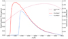 |
Fig. 1. Wavelength dependences of the throughputs T(λ) of the ACS/SBC F125LP and F140LP filters (solid curves, values on the left) and the extinction coefficient 10−0.4Aλ at E(B − V) = 0.22 (the dashed curve, values on the right), most probable for J1741. |
3. Data analysis
The SBC images in Figure 2 show a prominent extended structure and two point sources marked by 1 and 2. The extended structure is obviously an FUV counterpart of the Hα BSN. While the SBC images, centered on an outdated catalog position of J1741, do not fully cover the BSN, the offset had the happy accident of including a UV-bright field star (Source 2), which has allowed us to refine the HST astrometry. The archival Hα BSN image, obtained on 2018 August 6 at the 4.1 m Southern Astrophysical Research (SOAR) telescope with SOAR Adaptive Optics Module (SAM)2 (PI Roger Romani), is shown in the top right panel of Figure 2 (see also Romani et al. 2010; Auchettl et al. 2015).
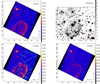 |
Fig. 2. FUV and Hα images of the field including J1741 and its BSN. Source 1 is the pulsar counterpart, Source 2 is the bright UV point source, used for astrometry. The arrows show the direction of the pulsar’s proper motion. Top left: F125LP image of the whole ACS/SBC FoV. The white contour shows the outer boundary of the Hα BSN from the SOAR image. Top right: SOAR/SAM Hα image of the BSN. The red cross shows the pulsar position. Bottom left: Same field as shown in the top left panel. Six areas within the white, yellow, and green contours were used for the flux measurements from the specific regions of the BSN (see Table 2); the background for this measurement was extracted from the areas within the corresponding cyan contours. Bottom right: F140LP image. |
The fainter point source in Figure 2 (Source 1 hereafter), located about 1 0–1
0–1 2 behind the bow shock apex, is the obvious candidate for the pulsar counterpart. As we show in the next subsection, this identification is supported by astrometric referencing of the HST FUV images.
3.1. Astrometry
The HST astrometric referencing can be obtained with the aid of the brighter Source 2, seen in both the F125LP and F140LP images. Its positions in the FUV images are measured with a high precision of about 1 mas.
Source 2 was also detected in the near-UV by the XMM-Newton Optical Monitor (OM) (Page et al. 2023) and the Swift Ultraviolet/Optical Telescope (UVOT) (Yershov 2015). It likely corresponds to Gaia DR3 source 4118158374505339904, with the ICRS coordinates α = 17:41:57.76052(4), δ = −20:53:43.5218(4)3 (at MJD 57388), proper motion μα = −4.7 ± 0.7 mas yr−1, μδ = −0.7 ± 0.4 mas yr−1, and magnitude mG = 19.88. The SOAR Hα image shows a very nearby (∼0.8 arcsec) northern neighbour (Gaia DR3 source 4118158374505339776) that could, in principle, also be considered as the Source 2 counterpart. That northern neighbor, however, is much redder (detected in the near-IR but not detected in the near-UV with the XMM-Newton OM and the Swift UVOT) and classified as a galaxy by Minniti et al. (2023). Therefore, Gaia DR3 source 4118158374505339904 is the only probable counterpart of Source 2.
With account for the proper motion, the Gaia coordinates of the Source 2 differ from the coordinates in the F125LP image by 1 09 and 0
 19 in RA and Dec, respectively. This means that the WCS of the F125LP image is offset from the Gaia WCS by about
  , which considerably exceeds the claimed HST pointing uncertainty of about 0
 1.4 For the F140LP image, these offsets are 1
 32 in RA and 0
 19 in Dec.
We applied the corresponding boresight corrections to the F125LP and F140LP images and obtained the following Source 1 coordinates: α = 17:41:57.221(1), δ = −20:54:13.66(2) in the F125LP image and α = 17:41:57.218(1), δ = −20:54:13.62(2) in the F140LP image. However, being based on “one-star astrometry”, these coordinates cannot be considered as precisely measured.
To prove that Source 1 is the pulsar counterpart, we compared these coordinates with the coordinates of the optical pulsar counterpart candidate detected by Mignani et al. (2016) with the VLT FORS2 in the bhigh and vhigh bands. We re-reduced these VLT images, obtained in 2015. To get an accurate astrometric solution, we used 15 stars from the Gaia DR3 catalog (Gaia Collaboration 2016, 2023). The coordinates of the reference stars at the epoch of the VLT observations were calculated using the cataloged proper motion values and the default cataloged coordinates at the 2016.0 reference epoch. For the bhigh image, we obtained the astrometric solution with uncertainties of 21 mas in RA and 20 mas in Dec, using the IRAF tasks imcentroid and ccmap. This allowed us to measure the coordinates of the pulsar counterpart candidate in bhigh image more accurately than it was done by Mignani et al. (2016). Accounting for the centroiding uncertainties of the candidate, we obtained its coordinates α = 17:41:57.268(3), δ = −20:54:12.91(4) at the epoch of the VLT observations (MJD 57156). Applying the pulsar’s proper motion (Auchettl et al. 2015), we obtain the predicted coordinates of the VLT candidate at the HST epoch (MJD 60107), α = 17:41:57.231(8) and δ = −20:54:13.63(8), which are consistent with the position of the Source 1 within ≈1σ uncertainties. It means that the VLT counterpart candidate is the same object as the FUV candidate if (and only if) its proper motion is the same as that of the pulsar. This virtually proves that the object is the pulsar counterpart.
The proper-motion shift of the pulsar between the epochs of 2015 and 2023 is demonstrated in Figure 3, which shows the pulsar vicinity in the F125LP and bhigh images. Circles in the images show the positions of the counterpart candidate at the epochs of 2015 (yellow in the left panel) and 2023 (red and yellow in the left and right panels, respectively). The shift between these positions is 1 00 ± 0
 06, in agreement with the pulsar’s proper motion shift of 0
 88 ±0
88 ±0 12.
12.
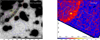 |
Fig. 3. VLT bhigh (MJD 57156) and HST F125LP (MJD 60107) images of the pulsar vicinity. The yellow rectangular regions were used for the measurements of surface brightness of the BSN apex in the HST and VLT images. The yellow circles show apertures used for the pulsar counterpart flux measurements in the HST and VLT images, while the yellow arrow shows the proper motion shift of the pulsar between the epochs of 2015 and 2023. The red circle in the VLT image shows the pulsar counterpart position from the HST F125LP image. The purple contours in the VLT image show the areas in which the background for pulsar counterpart was estimated, while the blue contour shows the background for the BSN apex. The white segment of annulus and the white box in the F125LP image show the background area for the pulsar counterpart and the BSN apex, respectively. In all cases a set of apertures (circular or rectangular) was randomly generated inside the background area to estimate the mean and standard deviation of the background count rate. The red line in the VLT image shows the position of BSN outer boundary from the HST image. |
An additional argument for the detected optical-FUV source being the true pulsar counterpart is its location with respect to the BSN. The distance between it and the bow shock apex, moving to south-east, is about 1 1 in both the F125LP and bhigh images. Thus, there remains no doubt that the optical-FUV source is indeed the pulsar counterpart.
3.2. Photometry
3.2.1. Pulsar
The pulsar counterpart count rates were measured in apertures of 8 pix (0 2) and 10 pix (0
 25) radii in the F125LP and F140LP images (Table 1), which contain 62% and 67% of point source counts, respectively (Avila & Chiaberge 2016). The background was extracted from the 135° sector of the annulus with inner and outer radii of 30 pix (0
 75) and 70 pix (1
 75) located behind the bow shock (right panel of Figure 3) in both SBC images. Because of proximity of bright background stars in the optical images, small apertures of 3 pix (0
 38) and 2 pix (0
 25) were used in the bhigh and vhigh images, respectively. The aperture correction in this case was determined with the aid of bright unsaturated stars. The background was extracted from the two small polygons behind the bow shock in the VLT images (left panel of Figure 3). We have to note that limited choice of background regions in the very crowded field could lead to an additional systematic error.
Pulsar photometry.
To evaluate the count rate uncertainties, we used the “empty aperture” approach (Skelton et al. 2014; Abramkin et al. 2022). The background count rates were measured in multiple apertures of the same shape and size as the source apertures, uniformly distributed in the background regions. We estimated the mean  and the variance σCbgd2 of the count rates inside the aperture, and calculated the net source count rate Cs and its uncertainty σs,
 (1)
(1)
where Ctot is the total count rate in the source aperture, texp is the exposure time, and g is the gain (g = 1 and 1.25 for the FUV and optical data, respectively). In the SBC images, we used a set of 1000 background apertures. For VLT photometry we used 50 and 35 background apertures in bhigh and vhigh images, respectively.
Photometric calibration for the optical bhigh and vhigh filters was applied using the mean night instrumental zeropoints and the atmospheric extinction coefficients5. Our vhigh and bhigh pulsar fluxes are slightly lower than those obtained by Mignani et al. (2016), while our uncertainties are significantly larger (see Table 1).
To convert the aperture-corrected pulsar’s count rate measured in a given SBC filter i, Cs, i/ϕi (where ϕi is the fraction of point source counts in the chosen aperture) to the mean flux density in that filter,
 (2)
(2)
we used the inverse sensitivity  obtained from the header keywords photflam and photplam in the data files. Note that the mean flux defined by Equation (2) is fully determined by the measured count rate and filter transmission Ti(λ) (see Figure 1), and it is not tied to a specific wavelength within the filter passband. It can be related to the “isophotal wavelength” λiso (Tokunaga & Vacca 2005), defined by the equation fν(λiso) = ⟨fν⟩, but λiso does depend on the spectral shape, and it cannot be determined from a count rate measurement in just one filter (unless the filter passband is very narrow). Moreover, the unique value of λiso can only be found if fν(λ) varies monotonously within the passband (as we expect for a pulsar FUV spectrum but not necessarily for a BSN spectrum).
3.2.2. Bow shock nebula
To explore the BSN emission in the F125LP, F140LP and bhigh images, we measured the count rates in six BSN regions, which we call Apex, Front, Back, Blob, Interior, and Half. These BSN regions and the corresponding background regions are shown in Figures 2 and 3, while their areas are presented in Table 2.
BSN photometry.
The brightest Apex region is a tiny  rectangle near the BSN apex (shown by the yellow rectangular contours in Figure 3). The background for this measurement was extracted from a
  rectangle ahead of the bow shock in the FUV images, where 1000 rectangular background apertures were generated applying the same “empty aperture” approach that we used for the pulsar photometry. In the very crowded bhigh field we extracted the background from a 6.9 arcsec2 polygon (see the left panel of Figure 3), where 85 background apertures were generated. Because of the crowded field, we were not able to accurately measure the count rates from the other BSN regions of the bhigh field.
The Front region includes the part of the flattish front of the BSN shell that was imaged onto the SBC detector. Some diffuse emission is seen throughout the entire ellipse-like BSN, with brightenings in its back part and in a compact region in the northern extreme of the BSN – the Back and Blob regions. The Interior region inside the closed BSN shell image possibly includes a contribution from the inner part of the 3D BSN. Finally, we measured the count rate from a half of the whole ellipse-like nebula seen in the FUV images (the Half region).
For the BSN photometry in the SBC filters, we measured the source count rates Cs for the six BSN regions as described above and, in addition, calculated mean surface brightnesses ℬs = Cs/As (see Table 2). For the BSN FUV photometry in the Front, Interior, and Half regions, we used sets of 20, 100, and 150 background apertures, respectively, placed in the corresponding background areas (see the bottom left panel of Figure 2). For the Back and Blob regions, we used sets of 50 background apertures placed in the same background area. We converted the source count rates to the mean flux densities ⟨fν⟩ using Equation (2) with ϕ = 1. If the BSN spectrum is a monotonous continuum, then there exists one isophotal wavelength within the filter passband, as described above. If, however, the BSN spectrum is dominated by spectral lines, then fν(λ) = ⟨fν⟩ at several values of λ, and the concept of the mean flux density becomes less useful.
4. Model fits
4.1. Pulsar optical-FUV spectral fits
We first fit the optical-FUV data with the simple absorbed PL model
 (3)
(3)
where ν0 and λ0 are the reference frequency and wavelength (we chose ν0 = 1015 Hz, which corresponds to λ0 = 3000 Å). The interstellar extinction A(ν) (or A(λ)) is proportional to the color excess E(B − V). For the DM-distance of 270 pc, resulting from the Galactic electron distribution model by Yao et al. (2017), the recent extinction map by Edenhofer et al. (2024) gives E(B − V) = 0.22. We also checked Lallement et al. (2022), Vergely et al. (2022), and Bayestar19 (Green et al. 2019) extinction maps and obtained the similar values. We will consider E(B − V)≃0.22 as the most probable color excess for d = 270 pc and use Cardelli et al. (1989) to connect A(λ) with the color excess. For this E(B − V), the wavelength dependence of the extinction coefficient 10−0.4A(λ) in the FUV range is shown in Figure 1.
We vary two model parameters (PL slope α and normalization fν, 0) at a fixed value of the color excess to minimize the χ2 statistic,
 (4)
(4)
where ⟨fν⟩i and σ⟨fν⟩i are the mean flux density and its error in the i-th filter; the mean model flux is given by Equation (2) in which fν is replaced by fνmod.
For the absorbed PL model, we obtained α = +1.0 ± 0.2 (i.e., photon index Γ = 1 − α = 0.0 ± 0.2), fν, 0 = 330 ± 40 nJy, with χ2 = 3.7 for 2 degrees of freedom (d.o.f.), for the color excess E(B − V) = 0.22. The best-fit spectrum and its uncertainties are shown by dash-dot and dotted blue lines in the left panel of Figure 4. Not only the fit is formally unacceptable, but also such large positive PL indices have not been seen in any other pulsar in the optical-UV.
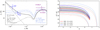 |
Fig. 4. Left: Fits of the optical-FUV spectrum. The dash-dotted and dotted blue lines show the best PL fit and its 68% uncertainties. The solid and dashed black lines show an example of a PL+BB fit with fixed α = −2, R15/d270 = 1 at E(B − V) = 0.22 and its components. Right: Confidence contours in the α–kT plane for R15/d270 = 1, at 68.3%, 99.7% confidence levels (for two parameters of interest). |
Therefore, we can assume that the FUV flux is, at least partly, due to thermal emission. We thus fit the optical-FUV flux densities with the PL+BB model
![Mathematical equation: $$ \begin{aligned} f_\nu ^\mathrm{mod} =\left[f_{\nu ,0} \left(\frac{\nu }{\nu _0}\right)^\alpha + \frac{R^2}{d^2} \pi B_\nu (T)\right]\times 10^{-0.4 A(\nu )}, \end{aligned} $$](/articles/aa/full_html/2025/04/aa52211-24/aa52211-24-eq38.gif) (5)
(5)
where d = 270d270 pc is the distance, T and R are the NS temperature and radius as seen by a distant observer, and Bν(T) is the Planck function. The best-fit parameters for the BB+PL model are kT = 48 ± 4 eV, α = −3.3 ± 2.2 (i.e., Γ = 4.3 ± 2.2),  nJy at the fixed values of E(B − V) = 0.22 and R15/d270 = 1 (where R = 15R15 km) with χ2 = 1.2 for 1 d.o.f.
The right panel of Figure 4 shows the 68.3% and 99.7% confidence contours (for two parameters of interest) for R15/d270 = 1 and three values of the color excess: E(B − V) = 0.21, 0.22, and 0.23. We see that the fits are almost insensitive to the spectral slope value at α ≲ −2, because of few data points. Therefore, we tried to fit the BB+PL model with the spectral slope fixed at α = −2. In this case, we obtained the following best-fit parameters: kT = 47 ± 4 eV, fν, 0 = 63 ± 15 nJy, χ2 = 1.6 for 2 d.o.f. at R15/d270 = 1, for E(B − V) = 0.22 (see the left panel of Figure 4).
For an alternative DM-distance of 380 pc, resulting from the Galactic electron distribution model by Cordes & Lazio (2002), the extinction map by Edenhofer et al. (2024) suggests a larger color excess, E(B − V) = 0.26. The larger distance and extinction lead to unrealistically high temperatures and/or thermally emitting areas derived from the optical-FUV fits, inconsistent with those obtained in X-rays. For instance, we got T ∼ 120 eV for R15/d380 ∼ 1 versus T ∼ 60 eV and R15/d380 ∼ 0.3 in X-rays (See Sect. 1). We thus adopt d = 270 pc and E(B − V) = 0.22 for further analysis.
4.2. Optical through X-ray spectrum of the pulsar
The pulsar surface temperature derived from the optical-FUV spectral fit is generally compatible with that obtained from the Chandra X-ray spectra using the same BB+PL emission model (Karpova et al. 2014; Auchettl et al. 2015). However, continuation of the PL component of this model obtained from the X-ray data alone overshoots the optical-FUV fluxes by several orders of magnitude. It means that the optical through X-ray nonthermal emission of the pulsar cannot be described by a single PL, but it can possibly be described by a broken PL (brPL) model,
 (6)
(6)
where E0 = 1 keV is the reference energy, Ebrk is the break energy, Γopt = 1 − αopt and ΓX = 1 − αX are photon indices at energies lower and higher than Ebrk, and the normalization KPL is the photon flux density at E = E0 for the low-energy branch (or its extrapolation).
To check this hypothesis and estimate the nonthermal and thermal model parameters, we fitted, using XSPEC spectral fitting package (ver. 12.13.0, Arnaud 1996), the FUV and optical data points together with the X-ray spectra obtained with the Chandra ACIS-S instrument (programs “A Legacy Study of the Relativistic Shocks of PWNe”, PI Roger Romani, and ”Constraining the Distance & Temperature of LAT PSR J1742–20, The Newly Discovered Nearby Middle-Aged Neutron Star”, PI Gregory Sivakoff) and reduced by Karpova et al. (2014). In our fits, we used the Tübingen-Boulder interstellar medium (ISM) absorption model (TBABS) with Wilms abundances (Wilms et al. 2000) in X-rays and the REDDEN interstellar extinction law (Cardelli et al. 1989) in the optical-UV. Following Zharikov et al. (2021) and Zyuzin et al. (2022), we used the python package emcee (Foreman-Mackey et al. 2013) to fit the data with the Markov chain Monte Carlo (MCMC) approach, using the affine invariant MCMC sampler (Goodman & Weare 2010). We utilized 1000 walkers and 50 000 steps for each of the tried models.
We used the hydrogen column density value,  , measured by Auchettl et al. (2015) from the PL spectral fit of the compact PWN in a 10″ vicinity of the pulsar, as a prior, while the color excess was fixed at E(B − V) = 0.22. The corresponding ratio
  , at AV = 3.1E(B − V), is in excellent agreement with the correlation NH, 21/AV = 1.79 ± 0.03 found by Predehl & Schmitt (1995), although this ratio is significantly lower than 2.87 ± 0.12 suggested by Foight et al. (2016). We started from fitting the absorbed brPL + BB model. The best fit is shown in the left panel of Figure 5. The BB temperature, kTBB = 51 ± 1 eV, is somewhat lower than those obtained from the X-ray-only fits, 58–65 eV (Karpova et al. 2014; Marelli et al. 2014; Auchettl et al. 2015), while it is compatible with the (rather uncertain) temperature range of ∼40–50 eV estimated above for the optical + FUV data. At the same time, the emitting sphere radius
  km at the distance d = 270 pc is larger than R = 3–5 km (recalculated for the same distance) from X-ray only fits. The break energy of the brPL component, Ebrk ≈ 0.5 keV, is in the soft X-ray range, where the BB component dominates. The brPL slopes, αopt = −0.04 ± 0.04 at E < Ebrk and αX = −1.60 ± 0.02 at E > Ebrk, correspond to the optical-FUV and X-ray parts of the pulsar’s nonthermal spectrum. The brPL slope in X-rays is within the range of −1.7 < αX < −1.6 found from the X-ray-only BB+PL fits, while αopt is at the upper end of the very broad interval of the PL slopes allowed by PL+BB fit of the optical-FUV spectrum (see Figure 4). The brPL normalization
  photons cm−2 s−1 keV−1 at 1 keV corresponds to extrapolation of the low-energy branch.
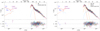 |
Fig. 5. Observed optical-FUV and X-ray spectra of J1741 fitted with the absorbed brPL + BB (left) and brPL + BB + BB (right) models. The blue and violet data points show the VLT optical and HST FUV data, respectively, while the seven separate X-ray data sets from Chandra observations (see Table 1 in Auchettl et al. (2015)) are shown in different colors. The solid red lines show the best-fit models (see text and Figure 6 for the best-fit parameters), whereas the red dashed, orange dot-dashed, and blue dotted lines show model components, as indicated in the legends. The fit residuals shown in the bottom subpanels are defined as χ ≡ (data − model)/error. |
With the reduced chi-square χred2 = 625/560 = 1.116 and reasonable fitting parameters, the fit with the brPL + BB model looks acceptable. However, the observed pulsations in soft (mostly thermal) X-rays with a pulsed fraction of ∼35%–40% (Marelli et al. 2014) mean that the temperature is not uniformly distributed over the NS surface (i.e., the brPL +BB model does not describe the phase-resolved X-ray data). Therefore, we considered a model with two thermal (BB) components: a cold BB component from the bulk of the NS surface and a hot BB component from small areas of the surface, presumably heated by the relativistic particles precipitating from the pulsar magnetosphere. The best fit gives  (versus 1.116 for the BB + brPL model), which means that the second thermal component is needed with probability of 99.99999 %, according to the F-test.
In the brPL + BB +BB fit the fitting parameters for the colder BB component,  eV and Rcold = (14.7 ± 1.1) km at d = 270 pc, are close to the BB parameters obtained from the BB + brPL fit. The brPL slopes,
  and αX = −1.66 ± 0.04, also do not show a substantial change. The hot BB component is characterized by kThot = (83 ± 5) eV and Rhot = (1.2 ± 0.3) km at d = 270 pc.
 |
Fig. 6. Posterior probability distributions for pairs of the fitting parameters for the absorbed BB + BB + brPL fit of the optical-FUV + X-ray data with 68% and 95% percentile contours. Marginalized 1D parameter distributions are shown with the median parameter values and 68% credible intervals. The vertical dashed lines correspond to 68% and 95% percentiles of the distributions. The BB normalization is defined as KBB = (R/10 km)2/(d/1 kpc)2, and the brPL normalization KPL is the photon flux of the low-energy component in units of 10−5 photons cm−2 s−1 keV−1 at 1 keV (see the text for all the notations). |
The best-fit spectrum for the BB + BB + brPL model is shown in the right panel of Figure 5, while the 1D and 2D posterior probability distributions with median values and 68% limits of the model parameters are presented in Figure 6. The BB normalization in Figure 6 is defined as KBB = R102/dkpc2, where R10 is the radius of equivalent emitting sphere in units of 10 km (for a distant observer), and dkpc is the distance in units of 1 kpc. Thus,  corresponds to Rcold = 14.7 ± 1.1 km at dkpc = 0.27. We see from the right panel of Figure 5 that the hot BB component dominates the spectrum in a rather narrow energy range, about 0.5–0.7 keV. Thus, adding the hot BB component does not significantly affect the overall fit, and it does not resolve the problem of the high pulsed fraction at E ≲ 0.5 keV, where the (cold) BB component dominates. More complicated (likely, multi-temperature) models for the thermal emission could help, but they require a phase-resolved spectral analysis, which is beyond the scope of this work.
4.3. Bow shock nebula
Since the F125LP and F140LP filters are rather broad, and the passband of F140LP is within the F125LP passband (see Figure 1), we have very little information on the FUV BSN spectrum. We do not even know whether the spectrum is dominated by spectral lines (like in the optical range) or by a continuum, or lines and continuum are similarly important. The only observational parameter available that may constrain the spectral shape for a BSN element is the ratio of count rates (or average brightnesses) in the two FUV filters, η ≡ CF125LP/CF140LP. Table 3 shows this ratio for the six BSN regions. The differences of the count rate ratios in different BSN regions are within their statistical uncertainties, with the weighted mean value  for the non-overlapping elements (first five lines in Table 3).
Properties of BSN regions.
If the spectrum of a BSN element is dominated by a continuum, which can be approximated by a PL in the FUV range (fν = fν, 0να for the unabsorbed spectrum), then we can, following Rangelov et al. (2016), use the measured η values to estimate, with the aid of stsynphot6, the range of allowed spectral slopes α, at fixed values of E(B − V). Then, for given α and extinction, we can calculate the normalization fν, 0 which gives the measured count rates. The calculated values of α and fν, 0 allow one to calculate the flux F = ∫fν dν in a range of FUV frequencies (or wavelengths) and estimate the FUV “isotropic luminosity”, L ≡ 4πd2F. Table 3 provides the ranges of α and flux intensity normalizations, as well as fluxes and luminosities in the 1250–1850 Å band. We see that the slopes are rather uncertain, particularly for small regions. The weighted mean slope for the five non-overlapping elements is  .
.
If spectral line(s) dominate the spectrum, then we need to know the number of the lines and their central wavelengths to estimate fluxes and luminosities of the BSN elements. The flux density of a line k with a width much narrower than the filter width can be approximated as fν, k = Fk δ(ν − νk), where Fk is the flux in the line, νk = c/λk, λk is the line’s central wavelength. The contribution of such a line in the count rate of the i-th filter is Ci(k) ∝ FkλkTi(λk), and the count rate ratio is
![Mathematical equation: $$ \begin{aligned} \eta = \left[\sum _k F_k \lambda _k T_{125}(\lambda _k)\right]\left[\sum _k F_k \lambda _k T_{140}(\lambda _k)\right]^{-1}\,, \end{aligned} $$](/articles/aa/full_html/2025/04/aa52211-24/aa52211-24-eq60.gif) (7)
(7)
where T125(λk) and T140(λk) are the throughputs in the F125LP and F140LP filters at λ = λk. In principle, the count rate ratio η could be provided by one spectral line centered at the wavelength where the ratio T125/T140 = η. For η = 1.62 ± 0.06 (the Half region), the central wavelength of such a hypothetical line is 1368–1369 Å, and the mean line intensity I = F/As = 2 × 10⁻¹⁶ erg cm−2 s−1 arcsec−2 provides the surface brightnesses ℬs = 0.045 and 0.028 counts s−1 arcsec−2 in the F125LP and F140LP filters, respectively. This corresponds to the observed flux F−14 ≡ F/(10−14 erg cm−2 s−1) = 2.9 from the Half region (F−14 ≈ 5.8 from the full, nearly elliptical BSN). However, as there are no strong lines at these wavelengths, there should be at least one line in the F140LP passband and one line in the 1230–1350 Å range. Without knowing the line wavelengths, we cannot estimate the energy flux and intensity from the two count rates available. We can, however, consider the above-estimated flux in the hypothetical line as close to a lower limit.
The observed Hα energy flux from the full J1741 BSN is  (Brownsberger & Romani 2014), which corresponds to the unabsorbed flux FHα, −14 ≈ 3.8. Although we do not know the true FUV spectrum of the BSN, the above estimates of the FUV flux demonstrate that it exceeds the Hα flux. For instance, assuming that the spectrum can be described by a PL model, we estimated the unabsorbed 1250–1850 Å flux FFUV, −14 ≈ 27 for the Half region (≈54 for the full BSN), at E(B − V) = 0.22, which corresponds to the FUV luminosity
  erg s−1. The unabsorbed FUV flux and luminosity exceed those in the Hα line by a factor of 14.
5. Discussion
The HST FUV observation presented here allowed us to to detect with high confidence the UV counterpart, and confirm the optical counterpart, of the middle-aged J1741 pulsar. In addition, we detected the FUV BSN created by this pulsar. Below we discuss the inferred properties of the J1741 pulsar and its BSN and compare them with the properties of similar objects.
5.1. The pulsar
Our analysis of the HST FUV and archival VLT optical data on the J1741 pulsar has shown that most likely the optical-UV emission of this pulsar consists of two components representing nonthermal emission from the pulsar magnetosphere and thermal emission from the NS surface. It is difficult to confidently constrain the PL slope of the optical-FUV nonthermal component with the currently available data in this range alone. Additional observations in the near-IR and near-UV are required to reliably constrain the PL slope and temperature of the bulk of the NS surface.
Adding X-ray archival data to the analysis allowed us to fit the multiwavelength spectrum of the pulsar with the brPL + BB or brPL + BB + BB models. In these models the low-energy part of the nonthermal emission, from the optical to the break energy of about 0.5 or 1.2 keV, is described by a hard PL with photon index Γopt ≈ 1.0–1.2 (−αopt ≈ 0–0.2), while one or two BB thermal components plus a soft PL component with ΓX ≈ 2.6–2.7 (−αX ≈ 1.6–1.7) are needed to describe the pulsar spectrum in X-rays up to 10 keV. According to these fits, the temperature of the bulk of the NS surface, kTcold ≈ 40–52 eV, is significantly lower than 60 ± 2 eV value obtained from the X-ray data alone (see Section 1). As can be seen from Figure 5 of Karpova et al. (2014), the lower temperature makes the position of J1741 in the NS temperature-age plane fully consistent with the predictions of the standard NS cooling models. The temperature of the hot BB component in the brPL + BB + BB fit, kThot ∼ 80 eV, could be ascribed to a small part of the NS surface, possibly heated by relativistic particles precipitating from the NS magnetosphere or by the anisotropic heat transfer from the NS interiors.
Although the spectral fits are formally acceptable, we have to note that they are hardly consistent with the high pulsed fraction of the (cold) thermal component (Marelli et al. 2014), at least for the locally semi-isotropic BB emission from NS surface elements. This suggests that the BB + BB model is too simplistic to describe the thermal emission from J1741. In particular, it seems quite plausible that, instead of two surface regions with different temperatures and emitting areas, there is a smooth temperature distribution over the NS surface caused by the anisotropic heat transfer in a strong magnetic field (Greenstein & Hartke 1983). For instance, if an NS possesses a dipole magnetic field near the surface, its magnetic poles are warmer than the magnetic equator, even without external heating of the poles by relativistic particles. According to Yakovlev (2021a,b), the BB + BB model can mimic thermal spectrum from an NS with such a temperature distribution, under the assumption that the surface elements emit semi-isotropic BB with the local temperatures. These models, however, do not reproduce the observed high pulsed fraction of thermal emission. The high pulsed fraction can be reached if there is a strong toroidal component of the magnetic field under the NS surface (Geppert et al. 2006; Igoshev et al. 2021).
A higher model pulsed fraction can also be obtained if one takes into account the anisotropy of local emission from a magnetized NS surface. Bombardment of NS polar regions by relativistic electrons or positrons not only additionally heats these regions, but it can also produce protons and α-particles in spallation reactions (i.e., a light-element plasma atmosphere can be formed above the polar caps) (Ho et al. 2007). The highly anisotropic photon emission emergent from such an atmosphere (Pavlov et al. 1994) can explain the high pulsed fraction of the hot thermal component.
The cold thermal component is expected to come from colder surface regions that can be formed by a condensed (liquid-like or solid-state) matter in a strong magnetic field (e.g., Medin & Lai 2007). The spectrum of its emission is not strongly different from the BB spectrum depressed by a constant factor (van Adelsberg et al. 2005; Pérez-Azorín et al. 2005), but the angular distribution of its specific intensity should be anisotropic. We are not aware of detailed investigation of pulsed emission from a rotating NS with a condensed surface (but see Pérez-Azorín et al. 2005). Consideration of more complicated surface emission models is, however, beyond the scope of this paper.
Since J1741 is a γ-ray pulsar, we can compare the optical through X-ray nonthermal spectrum with the γ-ray spectrum. Figure 7 shows the multiwavelength J1741’s spectral energy distribution (SED) from optical to γ-ray photon energies, using the Fermi LAT results (Abdollahi et al. 2020; Ballet et al. 2023). We see that the nonthermal spectrum has at least two spectral breaks, at ∼1 keV and ∼200 keV. It suggests that the nonthermal emission is not produced by a single physical mechanism, and it likely comes from distinct sites. We, however, cannot exclude that more observations in the IR-optical-UV range and more realistic models of thermal emission can significantly change the optical and X-ray PL slopes, so that, for instance, the optical PL may become softer while the X-ray PL may become harder (and maybe even dominated by the hot thermal emission in the Chandra/XMM-Newton range). However, it seems impossible to describe the nonthermal 1 eV – 100 MeV spectrum by a single PL.
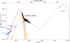 |
Fig. 7. SED for the unabsorbed optical through γ-ray emission from J1741. The cold BB, hot BB, and broken PL model components are shown by red-orange, orange, and blue lines, respectively, the corresponding shaded areas show the 1σ uncertainties of the model components in the ranges where the pulsar was observed. The purple lines and shaded area show the γ-ray model and its 1σ uncertainties, whereas the light purple shaded area shows the continuation of the γ-ray model toward lower energies. The blue solid line shows the best-fit model to the optical-UV and X-ray data. |
With a characteristic age of 386 kyr and distance ∼270 pc, the J1741 pulsar belongs to a small group of nearby, middle-aged pulsars detected in the FUV, which include Geminga, B0656+14, and B1055-52 (B0656 and B1055 hereafter), sometimes called the Three Musketeers (Becker & Truemper 1997). The multiwavelength spectrum of J1741 is compared with those of the Three Musketeers in Figure 8, while the spectral parameters of all the four pulsars are compiled in Table 4. Note that the spectral models used for fitting were not exactly the same for the four pulsars. The parameters of J1741 were obtained from a joint optical through X-ray fit with the brPL + 2BB model, while the X-ray and optical-UV spectra of B1055 and Geminga were fitted separately, with the PL + BB + BB and PL + BB models, respectively, and both models were applied to B0656 (with addition of an absorption feature at 0.5–0.6 keV). Therefore, in Table 4, the positions of the spectral break (Ebrk) in the nonthermal emission component are given only for J1741 and B0656.
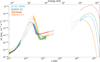 |
Fig. 8. SED for the unabsorbed IR through γ-ray emission from J1741 and other well-studied middle-aged pulsars. The IR through X-ray fit parameters for B1055-52, Geminga, and B0656+14 are taken from Posselt et al. (2023), Kargaltsev et al. (2005), Mori et al. (2014), Durant et al. (2011), and Arumugasamy et al. (2018). The γ-ray fit parameters are taken from Fermi LAT 14-Year Point Source Catalog (4FGL-DR4) Abdollahi et al. (2020), Ballet et al. (2023)). |
We see from Figure 8 that the phase-integrated multiwavelength spectra of the four middle-aged pulsars are qualitatively similar. All of them have prominent “thermal humps”, seen above the nonthermal spectrum from ∼5 eV to ∼2 keV. For all the four pulsars, these humps can be described by combinations of cold and hot BB components. The main contribution to the thermal humps comes from the cold components, with temperatures kTcold ∼ 40–70 eV, radii of equivalent emitting spheres Rcold ∼ 5–15 km, and bolometric luminosities Lcold ∼ (0.6–3.6)×1032 erg s−1. The Rayleigh-Jeans tails of the cold thermal component have been detected in the FUV (E ∼ 6–10 eV) for all the four pulsars. The FUV fluxes were included in the brPL + 2BB fits of the spectra of two of the four pulsars, B0656 and J1741, which resulted in somewhat different kTcold compared to X-ray-only fits.
We see from Table 4, that Tcold ∼ 42 eV, Rcold ∼ 15 km (for the estimated distance of 270 pc), and Lcold ∼ 0.9 × 1032 erg s−1, of J1741 are within the temperature and luminosity ranges for the Three Musketeers. As the radii of J1741, B0656, and Geminga are comparable with an expected NS radius, one can assume that the cold thermal emission comes from a substantial part of the NS surface and is likely powered by the heat supplied by hotter NS interiors. The temperatures and luminosities do not show a clear decrease with increasing the pulsars’ characteristic ages, but we should not forget that true ages may differ from characteristic ages, and the distances to three of the four pulsars are not well known, which affects the radius and, particularly, luminosity estimates.
Optical-FUV and X-ray properties of J1741 and the Three Musketeers.
For the cases where the optical-UV and X-ray spectra were fitted separately, the temperatures TFUV in Table 4 are brightness temperatures estimated from the measured FUV flux densities at an assumed (fixed) NS radius of 15 km and the best distance estimates available. Since fν ∝ (R/d)2T in the Rayleigh-Jeans regime, and the best-fit radii Rcold are smaller than assumed RFUV = 15 km for the Three Musketeers, it is not surprising that TFUV is lower than Tcold.
Additional hot BB components, with close temperatures kThot ∼ 80–200 eV, are seen in the X-ray emission of all the four middle-aged pulsars. The effective radii of J1741 and B0656, are close to each other, Rhot ∼ 1 km, but they are significantly larger than Rhot ∼ 200 m and 45 m for B1055 and Geminga, respectively. The corresponding bolometric luminosities, Lhot ∼ (0.4–30)×1030 erg s−1, also show a strong scatter, with the Geminga’s luminosity being an obvious outlier. The luminosities do not show correlation with the spindown power, as would be expected for heating by magnetospheric particles, but there is hint of positive correlation with Lcold (at least if we exclude the outlier Geminga). This suggests that the anisotropic heat transfer from the NS interior indeed plays a role in heating the polar regions.
The ratio of the hot BB and cold BB temperatures, obtained from the phase-averaged fits, Thot/Tcold ≈ 2.0 for J1741, is close to 2.4 for B1055 and 1.9 for B0656, but it is substantially lower than 4.4 for Geminga. According to Yakovlev (2021a), the anisotropic heat transfer alone cannot explain such high temperature ratios for a dipole magnetic field (typical values do not exceed 1.2 in those calculations). This means that either there is an additional heating mechanism of the hot regions or the magnetic field is different from a centered dipole (e.g., there is a strong toroidal component under the NS surface). Different temperature ratios of the four pulsars can come from a combination of differences in the bulk temperatures distributions, hot spot temperatures (influenced by different magnetic field topology and strengths), and pulsar geometries (rotation-magnetic axes inclinations and viewing angle) as well as possible occultations of the surface by plasma-filled patches in the magnetopshere (Kargaltsev et al. 2012). Different pulsed fractions in the thermal components, from ∼36% for J1741 (Marelli et al. 2014) to ∼65% for B1055 (Vahdat et al. 2024) are additional observational manifestations of these effects. Nevertheless, it is remarkable that the temperature ratios for the three pulsars are in a relatively narrow range around 2 even if we take into account their variations with the pulsar rotation phase (e.g., Thot/Tcold varies from 1.9 ± 0.2 to 2.7 ± 0.2 for B1055 and from 1.8 ± 0.2 to 2.2 ± 0.3 for B0656; Vahdat et al. 2024; Arumugasamy et al. 2018).
The distance-independent ratios of BB radii and bolometric luminosities for the cold and hot components are also similar for J1741, B1055, and B0656 (Rhot/Rcold ∼ Lhot/Lcold ∼ 0.04–0.10), but they are significantly smaller for Geminga (0.004 and 0.006 for the radii and luminosties ratios, respectively). These ratios are much smaller than calculated by Yakovlev (2021a) for the anisotropic heat transfer in a dipole magnetic field, which can be considered as an additional argument against such a simplified picture. Rigoselli et al. (2022) have noticed that six rotation powered pulsars of different ages whose thermal spectra are well described by the double BB model, including the Three Musketeers except of Geminga, occupy a remarkably compact region in the (Thot/Tcold)–(Rhot/Rcold) plane. This may imply similar surface temperature maps for these pulsars independently of their ages. J1741 obviously joins to this group.
All the four pulsars show qualitatively similar nonthermal spectra in the optical to X-ray range (Figure 8). If fitted by a PL model fν ∝ να = ν1 − Γ separately in the two ranges, the slope α is more negative in X-rays than in the optical (e.g., αopt − αX = ΓX − Γopt ∼ 0.2–0.4 for the Three Musketeers). It means that the nonthermal spectrum can be fitted with a broken PL in the optical through X-ray range, with a break energy Ebr between UV and hard X-rays. The break energy is rather uncertain for the Three Musketeers because the slope differences are small (see the example of B0656 in the last column of Table 4), but it is more certain for J1741, for which αopt − αX = 1.49 ± 0.08. This large value is due to the unusually steep X-ray PL slope, ΓX ≈ 2.7 versus 1.3–1.8 for the Three Musketeers, which is particularly well seen in Figure 8. The large ΓX is an outlier not only in the small sample of four pulsars but also among a large sample of pulsars with similar parameters, such as spindown power or characteristic age (see Figures 3 and 4 in Chang et al. 2023).
Similar to the other spectral parameters, the X-ray PL slope (photon index) varies with rotational phase. The relatively narrow photon index range in the phase-resolved spectra of J1741 (ΓX ∼ 2.3–2.8; Marelli et al. 2014) slightly overlaps with the respective ranges of B1055 (ΓX ∼ 1.5–2.5; Vahdat et al. 2024), Geminga (Γx ∼ 1.6–2.2; Mori et al. 2014), and B0656 (ΓX ∼ 1.5–2.3; Arumugasamy et al. 2018). A possible explanation for the J1741’s offset ΓX values and the relatively large ranges spanned by the photon indices of the Three Musketeers could come from different pulsar geometries that allow one to ‘see’ different parts of nonthermal emission regions around the pulsar. There is also the possibility that the J1741 spectrum has another phase-dependent thermal component, invisible with the current count statistics. However, our attempts to describe the high energy spectral tail by an extra BB component instead of the PL led to unacceptable fits. A deeper, phase-resolved X-ray study of J1741 could clarify this.
We see from Figure 8 that the nonthermal X-ray spectra do not connect smoothly with the γ-ray spectra for all the four pulsars. It could indicate that the X-rays and γ-rays come from different sites in the magnetosphere and/or are produced by different emission mechanisms. This inference is less certain for J1741 and B1055, which have not been observed in hard X-rays (above ∼10 keV).
We also see that the SEDs of the four pulsars reach their maxima in γ-rays, at energies from ∼100 MeV for B0656 to ∼2 GeV for Geminga. This implies that the most efficient conversion of the pulsar rotation energy to radiation occurs in γ-rays. The efficiency in a spectral band b is usually defined as ηb = Lb/Ė, where Lb is the (distance-dependent) luminosity in the band. Comparing the efficiencies ηγ estimated for the 0.1–100 GeV band (Table 4), we see that Geminga is the most efficient emitter in this band, B1055 and J1741 are intermediate ones, while B0656 has the lowest efficiency, in accord with the SEDs in Figure 8. In the optical-FUV (1–10 eV) and X-ray (1–10 keV) bands (where the efficiencies are lower than in γ-rays by about five and three orders of magnitude, respectively), J1741 seems to be the most efficient emitter among the four pulsars. Besides the obvious uncertainties due to uncertain distances, we have to note, however, that the nonthermal luminosity estimate of J1741 in the 1–10 eV band is based on the optical + X-rays fit with the brPL + 2BB model involving only four data-points in this band. New observations in the near-IR and near-UV are needed to add more data-points and confirm the high efficiency of J1741 in the optical-FUV band.
5.2. The bow shock nebula
The J1741 BSN, detected in our FUV observation for the first time, is one of only nine detected Balmer-dominated BSNe, best-studied in the Hα emission (Romani et al. 2010; Brownsberger & Romani 2014). The paucity of Balmer-dominated BSNe indicates that most pulsars move in an ionized ISM. The J1741’s BSN is visible in the VLT bhigh image due to the Hβ and Hγ emission lines (Mignani et al. 2016; see also Figure 3). We found no differences in the shape and size of the FUV and Hα BSNe, moving together with the pulsar. The BSN is confined within a closed shell, resembling an ellipse with a flattened back, elongated perpendicular to the proper motion direction. In the high-resolution SOAR and HST images (Figure 2) we see a “bulge” at the sharp, bright front of the shell, with a hint of continuation of the bulge boundary into the (projected) BSN interior. The bulge and its continuation (if confirmed with deeper high-resolution observations) can be interpreted as a forward bow shock, while the rest of the BSN could be a “bubble”, similar to those in the famous Guitar BSN (de Vries et al. 2022, and references therein). There is also a slight hint of a bent “trail” in the northeast direction, starting from the Blob region, which might be interpreted as a northwest boundary of a second “bubble”.
This interpretation of the BSN structure is supported by the comparison of the X-ray PWN and the FUV/Hα BSN shown in Figure 9. We see that the compact component of the X-ray PWN, presumably created by the shocked pulsar wind, is seen almost up to the BSN (bulge) apex ahead of the moving pulsar, as expected (some X-ray counts ahead of the apex are due to the wings of the pulsar’s PSF). However, this compact PWN behind the pulsar, elongated along the pulsar motion direction, is much narrower than the BSN. On the other hand, the possible boundaries of the bulge continuation, shown by dashed green curves in the inset of Figure 9, are much closer to the compact X-ray PWN component, as expected from simulations of nebulae created by supersonically moving pulsars (e.g., Bucciantini et al. 2005).
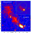 |
Fig. 9. Comparison of the J1741 X-ray PWN and Hα-FUV BSN shapes. The green contour shows the outer boundary of the Hα BSN as imaged by SOAR (see Figure 2), which virtually coincides with outer boundary of the FUV BSN, overlaid on the Chandra ACIS-S 0.7–8 keV image. The large-scale Chandra image is smoothed with a 5 pixel Gaussian kernel, while the zoomed-in 28″ × 26″ image of the compact PWN in the inset is shown without smoothing. The green dashed curves show the continuation of the bulge into the inner BSN region. The black cross shows the pulsar position. |
The J1741 BSN is only the third FUV BSN detected, and the first BSN associated with a middle-aged pulsar7. In Table 5 the properties of the J1741 FUV BSN are compared with those of the previously detected BSNe of the nearby millisecond pulsars J0437–4715 (Rangelov et al. 2016) and J2124–3358 (Rangelov et al. 2017), which we denote J0437 and J2124 hereafter. The spin-down powers Ė of these millisecond pulsars are only slightly lower than that of J1741, and all the three pulsars have been detected in the GeV γ-ray range.
Properties of the three known FUV BSNe.
At first glance, the closed-shell shape of the J1741 BSN looks drastically different from those of the two other BSNe. The J0437 BSN looks like a classic bow shock, whose shape is excellently described by a simple equation (Wilkin 1996). The forward part of the J2124 BSN resembles the bow shock of J0437, but the brightness distribution is asymmetric with respect to the proper motion direction, and the bow shock narrows behind the pulsar, apparently forming a bubble with a hint of a Guitar-like structure (Brownsberger & Romani 2014). The difference of the shapes of the BSN images may be associated with different geometries of the pulsar wind outflow, different local ISM pressures and/or magnetic fields, and different inclinations of the pulsar’s velocity to the line of sight (possibly the smallest for J1741).
Romani et al. (2010) suggested that the transverse elongation of the J1741 BSN is due to the pulsar wind being concentrated in the equatorial plane of the rotating pulsar whose spin axis is aligned with the pulsar’s velocity. However, if our assumption that only the bulge of the J1741 BSN is the actual forward bow shock is correct, then the apparent difference with the two other FUV/Hα BSNe could be explained, at least partly, by the projection effect: if the velocity vector is close to the line of sight, one will naturally get an observed shape, irrespective to the spin-velocity alignment. This would imply that the actual pulsar’s velocity can significantly exceed its transverse velocity, v⊥ ≈ 140d270 km s−1, and the actual lengths of structures aligned with the velocity vector, such as the ∼10″ (≃4.0 × 1016 cm in the sky projection) length of the compact PWN component, are significantly longer. Deeper FUV imaging would be most useful to examine this interpretation and estimate the velocity and the lengths more accurately.
We see from Table 5 that the J1741 BSN has the smallest projected distance between the pulsar and the forward bow shock apex, la, ⊥ = 4.4 × 10¹⁵d270 cm, which is factors of 5.2 and 3.4 smaller than for the J0437 and J2124 BSNe, respectively. For an isotropic pulsar wind, the distance la to the bow shock front apex measured along the velocity vector slightly exceeds the standoff distance, where the ram pressures of the ISM and the pulsar wind balance each other (e.g., Brownsberger & Romani 2014; Reynolds et al. 2017): la ≈ 1.3(ξwĖ/4πcρv2)1/2, where ξw is the fraction of Ė that powers the pulsar wind, ρ is the mass density of the ambient ISM, v = v⊥/sin i is the pulsar velocity, and i is the velocity inclination with respect to the line of sight. The larger J1741’s projected velocity together with a smaller inclination i and/or a higher ISM density could explain the observed ratios of distances la, ⊥, but an anisotropic pulsar wind could be another factor.
The FUV BSN of J1741 looks brighter than those of J0437 and J2124. For instance, the (distance-independent) mean surface brightness in the F125LP image of the Front region of J1741, ℬs = 110 ± 2 cnts/(ks arcsec2), is 2.7 and 11 times higher than those of apex regions of J0437 and J2124 (the only regions for which ℬs was measured in those BSNe). The brightness ratios would become a factor of ∼4 larger if we account for the different ISM extinctions towards the pulsars (see Table 5). The high brightness of the J1741 FUV BSN makes it particularly suitable for FUV spectroscopy.
It is more difficult to compare the FUV count rates from entire BSNe because only parts of the J0437 and J2124 FUV BSNe were imaged in FUV. However, assuming that the FUV brightness distribution is similar to that in Hα, we crudely estimated that if the total count rate of the entire J0437 FUV BSN were measured, it would be a factor of about two higher than the count rate for the entire J1741 BSN (e.g., ≈13 cnts/s in F125LP – see Table 2). Similar estimates for the faint J2124 BSN are even more uncertain, but most likely its total FUV count rate would be somewhat lower than that of the J1741 BSN.
It would also be interesting to compare the FUV energy fluxes and luminosities of the three FUV BSNe. Accurate estimates for these quantities require knowledge of their FUV spectra, but all the spectral information is contained in the count rates in only two filters, F125LP and F140LP, with the passband of the latter being within the passband of the former. These count rates and, particularly, their ratio η (see Tables 3 and 5) can be used to estimate parameters of an assumed spectral model, as well as the FUV fluxes and luminosities (Rangelov et al. 2016). However, the fluxes and luminosities may be significantly different for spectra dominated by emission lines (e.g., from atoms or ions excited in passage of the bow shock) or a continuum (e.g., the continuum component of thermal emission from the shocked plasma or synchrotron radiation from electrons accelerated between the forward bow shock and the PWN termination shock, as suggested by Bykov et al. 2017).
Assuming a continuum PL spectrum, in Section 4.3 we estimated the PL slope α = −1.0 ± 0.7 and the unabsorbed FUV (1250–1850 Å, or 6.70–9.92 eV) energy flux FFUV, −14 ≈ 54 from the entire J1741 BSN. This corresponds to the observed flux  . Since η = 1.6 ± 0.1 is the same for J0437 and J1741 BSNe, we can assume the same spectral slopes and estimate that the absorbed energy flux from the entire J0437 BSN is ∼2 times higher than from the J1741 BSN. A similar flux ratio can be obtained if we scale the FUV flux from the J0437 BSN apex region, reported by Rangelov et al. (2016), and correct the error in the previous SBC flux calibration, reported by Avila et al. (2019), which resulted in ∼27% lower flux for a given count rate in the F125LP filter. Assuming E(B − V) = 0.22 for J1741, and E(B − V) = 0.05 for J0437, the full J1741 BSN luminosity, LFUV ≈ 4.7 × 1030d2702 erg s−1, is a factor of 5–7 higher than the full J0437 FUV BSN luminosity. Estimates of the full J2124 nebula observed flux and luminosity are, again, very uncertain, but likely both the total observed flux and the total FUV luminosity are lower than those of the entire J1741 BSN. The highest FUV luminosity of the J1741 BSN can be partly associated with the highest spin-down power of the J1741 pulsar and/or a higher ambient ISM density, but the dependence on these and other parameters depends on the BSN emission model.
Given the virtually coinciding images of the FUV and Hα BSNe, the hypothesis of the FUV BSN spectra being dominated by emission lines may look more plausible. Unfortunately, we can only guess which lines give a significant contribution. Obviously, it could only be strong lines of abundant elements. Since there are no H I or He I lines in this FUV range, one could consider, for instance, the Balmer-alpha line of He II, at ≈1640 Å (7.56 eV) or the strong C IV resonance line with fine structure components at 1548.19 and 1550.77 Å (around 8.00 eV). It is, however, difficult to explain lines of ionized species, particularly the highly ionized carbon. Since the BSNe are seen in Hα, the ISM should be mostly neutral ahead of them. It means that the initially neutral atoms, which can easier penetrate through the shock, should be ionized after passing through the shock, before their ions are excited to produce the lines. This may require too high temperatures behind the forward shock and may lead to a FUV BSN brightness distribution different from the Hα BSN brightness distribution, which has not been detected so far. On the other hand, Romani et al. (2010) report a few (forbidden) lines of once-ionized nitrogen, oxygen, and sulfur at optical wavelengths, so one can assume that lines of ionized elements can also be seen in the FUV J1741 BSN. To resolve this problem, BSN FUV spectroscopy is required, supported by realistic BSN models.
Another option could be FUV emission of molecular hydrogen, possibly due to Lyα fluorescence (see, for example, Wood et al. 2001; France et al. 2012 and Martin et al. 2007). However, the probability that three of the few pulsars observed in FUV are in molecular clouds seems to be very low.
One could also consider continuum emission due to the two-photon 2s → 1s transition in hydrogen atoms8. Using an analytical approximation for the two-photon emission spectrum (Nussbaumer & Schmutz 1984) and the F125LP throughput, we found that in order to explain the observed count rate (e.g., for the Half region of the BSN) by two-photon emission, the ratio of the number of photons emitted by this mechanism to the number of Hα photons should be about 11–12, assuming E(B − V) = 0.22. Such a ratio is significantly higher than ≲2 predicted by Kulkarni & Shull (2023) for low-velocity (vs≲ 70 km s−1) shocks. This ratio should be even lower for the high-velocity J1741 BSN. Therefore, it is very unlikely that two-photon decay is the main source of the FUV emission.
At the wavelengths of the mentioned He II and C IV lines the F125LP and F140LP throughputs are very close to each other (see Figure 1). Therefore, there should be at least one other line (or/and a continuum) in the ≈1230–1360 Å (9.12–10.09 eV) range in order to be consistent with the count rate ratio η > 1. Plausible candidates are the line complexes of OI lines at 1302–1306 Å (9.49–9.52 eV), C I lines around 1277 Å (9.72 eV), and N I lines around 1243 Å (9.98 eV). Only FUV spectroscopy can convincingly show which (if any) of these lines are present in the BSN emission.
As we still do not know the wavelength(s) and strength(s) of the putative lines, the flux and luminosity estimates are highly uncertain in a line-dominated FUV BSN spectrum. As we discussed in Section 4.3, we can only estimate conservative lower limits on the observed FUV flux,  , and luminosity,
  erg s−1. The lower limits on the line-dominated FUV flux translate into the lower limit of 2.5 on the observed (absorbed) FUV-to-Hα flux ratio while the ratio of the unabsorbed fluxes (and luminositie) is > 8. These limits are about 1.6–1.8 lower than the flux ratios, 4.1 and 14 for the observed and unabsorbed fluxes, respectively, that follow from the above-estimated fluxes for the PL spectrum model.
Similar excesses of FUV flux over Hα flux were obtained for the two other BSNe known (Rangelov et al. 2016, 2017). For instance, for the PL model of the J0437 BSN, the absorbed (unabsorbed) FUV flux is a factor of 5–7 (6–9) higher than the Hα flux. For the J2124 BSN, the ratio of unabsorbed fluxes, FFUV/FHα ≈ 3, for a flat fλ spectrum, but a factor of up to two higher values are not excluded. If the FUV spectra of the J0437 and J2124 BSNe are line-dominated, the FFUV/FHα ratios could be lower, but they remain > 1.
Since the photon energies in the FUV range, ∼(6.7–10) eV, exceed the energy 1.889 eV of Hα photons by a factor of about 3.5–5.3, the “photon luminosities” of the FUV and Hα BSNe are very close to each other. It is difficult to reconcile this finding with the line-dominated model of the FUV BSN spectra because it would require extremely high abundances of chemical elements responsible for the lines. We believe that most likely the FUV BSN emission is produced in a hot shocked plasma flow behind the bow shock, whose spectrum contains both a continuum component and spectral lines. Relative contributions of these component can hardly be inferred without modeling and further observations.
We can summarize our main findings on the J1741 and the two other FUV BSNe as follows:
-
The three detected FUV BSNe (as well as their Balmer-line counterparts) are created by pulsars with very different periods and ages, but with close spindown powers, Ė = (5.5–9.5)×1033 erg s−1, and transverse velocities v⊥ in the range of 100–150 km s−1. All three pulsars were detected in GeV γ-rays.
-
There are many pulsars with similar Ė and v⊥ that do not show BSNe, neither in FUV nor in Hα, which means that these parameters alone are not responsible for the presence of a BSN. Apparently, local ISM properties, such as density, pressure, and degree of ionization, are more important for BSN formation.
-
No FUV BSNe have been detected without Balmer-line counterparts. This implies the presence of neutral hydrogen atoms (cold ISM) ahead of the forward shock, which become heated and excited in the shock passage. The residual neutral hydrogen behind the shock front cannot be responsible for the observed FUV emission, but emission from a partly ionized plasma (e.g., bremsstrahlung) can provide a significant contribution.
-
All the FUV BSNe are spatially coincident with their Balmer-line counterparts, and the brightness distributions within the Balmer-line and FUV BSNe look similar. It suggests that they are created by similar processes, such as emission from a partly ionized plasma behind the forward shock.
-
We are not aware of Balmer-line BSNe without FUV counterparts, but six of the nine known Hα BSNe have not been imaged in the FUV.
-
The FUV BSN luminosities, LFUV∼(1–5)×1030 erg s−1, possibly correlate with Ė. They exceed the Hα luminosities by a factor of 3–14 for all three BSNe. This means that the FUV emission is not dominated by spectral lines because it would require unrealistically high abundances of elements heavier than hydrogen.
-
We presume that the FUV BSN emission comes from the ISM heated and ionized while passing through the forward bow shock. Its FUV spectrum likely includes both the continuum component and emission lines of abundant elements that can be studied in deep spectroscopic observations.
To conclude, the nature of the FUV BSNe remains very puzzling. To understand it, spectroscopic observations of the known FUV BSNe and a search for new FUV BSNe, supplemented by realistic models of these objects, are needed.
To the best of our knowledge, the image and its analysis have not been published. We took the data from the NOIRLab Astro Data Archive and reduced them.
Numbers in parentheses denote 1σ uncertainties relating to the last significant digits.
The Three Musketeers, whose pulsar properties are very similar to those of J1741 (see Table 4), show neither FUV nor Hα BSNe, indicating high ionization of the ISM around these pulsars. Moreover, their X-ray PWNe are drastically different from each other (Posselt et al. 2017; Bîrzan et al. 2016; Posselt et al. 2015) and from the J1741 PWN. The differences can be associated with different geometries of their pulsar winds and/or different local ISM properties.
We thank Marten van Kerkwijk for reminding us of this possibility.
Acknowledgments
Support for program #17155 was provided by NASA through a grant HST-GO-17155 from the Space Telescope Science Institute, which is operated by the Association of Universities for Research in Astronomy, Inc., under NASA contract NAS 5-26555. The work of V. A. was supported by the Russian Science Foundation grant 24-12-00320, https://rscf.ru/project/24-12-00320/. The work of Y. S. was partially supported by the baseline project FFUG-2024-0002 of the Ioffe Institute. We are grateful to Roger Romani for useful suggestions. We thank A. V. Karpova and D. A. Zyuzin for providing the reduced Chandra data. We express our thanks to the referee Marten van Kerkwijk for careful reading of the manuscript and thoughtful remarks and suggestions. This work has made use of data from the European Space Agency (ESA) mission Gaia (https://www.cosmos.esa.int/gaia), processed by the Gaia Data Processing and Analysis Consortium (DPAC, https://www.cosmos.esa.int/web/gaia/dpac/consortium). Funding for the DPAC has been provided by national institutions, in particular the institutions participating in the Gaia Multilateral Agreement. This research has made use of data obtained from the Chandra Data Archive provided by the Chandra X-ray Center (CXC). This research made use of the following software: IRAF (Tody 1986, 1993), XSPEC (Arnaud 1996), DrizzlePac (https://www.stsci.edu/scientific-community/software/drizzlepac), EsoRex (ESO CPL Development Team 2015), and Python packages Matplotlib (Hunter 2007), emcee (Foreman-Mackey et al. 2013), NumPy (Harris et al. 2020), Astropy (Astropy Collaboration 2022)
References
- Abdo, A. A., Ackermann, M., Ajello, M., et al. 2009, Science, 325, 840 [Google Scholar]
- Abdollahi, S., Acero, F., Ackermann, M., et al. 2020, ApJS, 247, 33 [Google Scholar]
- Abramkin, V., Pavlov, G. G., Shibanov, Y., & Kargaltsev, O. 2022, ApJ, 924, 128 [NASA ADS] [CrossRef] [Google Scholar]
- Arnaud, K. A. 1996, in Astronomical Data Analysis Software and Systems V, eds. G. H. Jacoby, & J. Barnes, ASP Conf. Ser., 101, 17 [NASA ADS] [Google Scholar]
- Arumugasamy, P., Kargaltsev, O., Posselt, B., Pavlov, G. G., & Hare, J. 2018, ApJ, 869, 97 [NASA ADS] [CrossRef] [Google Scholar]
- Astropy Collaboration (Price-Whelan, A. M., et al.) 2022, ApJ, 935, 167 [NASA ADS] [CrossRef] [Google Scholar]
- Auchettl, K., Slane, P., Romani, R. W., et al. 2015, ApJ, 802, 68 [NASA ADS] [CrossRef] [Google Scholar]
- Avila, R. J., & Chiaberge, M. 2016, Photometric Aperture Corrections for the ACS/SBC, Tech. rep. [Google Scholar]
- Avila, R. J., Bohlin, R., Hathi, N., et al. 2019, SBC Absolute Flux Calibration, Tech. rep. [Google Scholar]
- Ballet, J., Bruel, P., Burnett, T. H., Lott, B., & The Fermi-LAT collaboration 2023, ArXiv e-prints [arXiv:2307.12546] [Google Scholar]
- Becker, W., & Truemper, J. 1997, A&A, 326, 682 [Google Scholar]
- Bîrzan, L., Pavlov, G. G., & Kargaltsev, O. 2016, ApJ, 817, 129 [CrossRef] [Google Scholar]
- Brownsberger, S., & Romani, R. W. 2014, ApJ, 784, 154 [NASA ADS] [CrossRef] [Google Scholar]
- Bucciantini, N., Amato, E., & Del Zanna, L. 2005, A&A, 434, 189 [NASA ADS] [CrossRef] [EDP Sciences] [Google Scholar]
- Bykov, A. M., Amato, E., Petrov, A. E., Krassilchtchikov, A. M., & Levenfish, K. P. 2017, Space Sci. Rev., 207, 235 [CrossRef] [Google Scholar]
- Camilo, F., Ray, P. S., Ransom, S. M., et al. 2009, ApJ, 705, 1 [NASA ADS] [CrossRef] [Google Scholar]
- Cardelli, J. A., Clayton, G. C., & Mathis, J. S. 1989, ApJ, 345, 245 [Google Scholar]
- Chang, H.-K., Hsiang, J.-Y., Chu, C.-Y., et al. 2023, MNRAS, 520, 4068 [NASA ADS] [CrossRef] [Google Scholar]
- Cordes, J. M., & Lazio, T. J. W. 2002, ArXiv e-prints [arXiv:astro-ph/0207156] [Google Scholar]
- de Vries, M., Romani, R. W., Kargaltsev, O., et al. 2022, ApJ, 939, 70 [NASA ADS] [CrossRef] [Google Scholar]
- Durant, M., Kargaltsev, O., & Pavlov, G. G. 2011, ApJ, 743, 38 [NASA ADS] [CrossRef] [Google Scholar]
- Edenhofer, G., Zucker, C., Frank, P., et al. 2024, A&A, 685, A82 [NASA ADS] [CrossRef] [EDP Sciences] [Google Scholar]
- ESO CPL Development Team 2015, Astrophysics Source Code Library [record ascl:1504.003] [Google Scholar]
- Foight, D. R., Güver, T., Özel, F., & Slane, P. O. 2016, ApJ, 826, 66 [Google Scholar]
- Foreman-Mackey, D., Hogg, D. W., Lang, D., & Goodman, J. 2013, PASP, 125, 306 [Google Scholar]
- France, K., Schindhelm, R., Herczeg, G. J., et al. 2012, ApJ, 756, 171 [NASA ADS] [CrossRef] [Google Scholar]
- Gaia Collaboration (Prusti, T., et al.) 2016, A&A, 595, A1 [NASA ADS] [CrossRef] [EDP Sciences] [Google Scholar]
- Gaia Collaboration (Vallenari, A., et al.) 2023, A&A, 674, A1 [NASA ADS] [CrossRef] [EDP Sciences] [Google Scholar]
- Geppert, U., Küker, M., & Page, D. 2006, A&A, 457, 937 [NASA ADS] [CrossRef] [EDP Sciences] [Google Scholar]
- Goodman, J., & Weare, J. 2010, Commun. Appl. Math. Comput. Sci., 5, 65 [Google Scholar]
- Green, G. M., Schlafly, E., Zucker, C., Speagle, J. S., & Finkbeiner, D. 2019, ApJ, 887, 93 [NASA ADS] [CrossRef] [Google Scholar]
- Greenstein, G., & Hartke, G. J. 1983, ApJ, 271, 283 [NASA ADS] [CrossRef] [Google Scholar]
- Harris, C. R., Millman, K. J., van der Walt, S. J., et al. 2020, Nature, 585, 357 [NASA ADS] [CrossRef] [Google Scholar]
- Hartman, R. C., Bertsch, D. L., Bloom, S. D., et al. 1999, ApJS, 123, 79 [CrossRef] [Google Scholar]
- Ho, W. C. G., Kaplan, D. L., Chang, P., van Adelsberg, M., & Potekhin, A. Y. 2007, MNRAS, 375, 821 [CrossRef] [Google Scholar]
- Hunter, J. D. 2007, Comput. Sci. Eng., 9, 90 [NASA ADS] [CrossRef] [Google Scholar]
- Igoshev, A. P., Hollerbach, R., Wood, T., & Gourgouliatos, K. N. 2021, Nat. Astron., 5, 145 [Google Scholar]
- Kargaltsev, O. Y., Pavlov, G. G., Zavlin, V. E., & Romani, R. W. 2005, ApJ, 625, 307 [NASA ADS] [CrossRef] [Google Scholar]
- Kargaltsev, O., Durant, M., Misanovic, Z., & Pavlov, G. G. 2012, Science, 337, 946 [Google Scholar]
- Kargaltsev, O. Y., Posselt, B., Pavlov, G. G., et al. 2022, The legacy UV survey of 28 pulsars, HST Proposal. Cycle 30, ID. 17155 [Google Scholar]
- Karpova, A., Danilenko, A., Shibanov, Y., Shternin, P., & Zyuzin, D. 2014, ApJ, 789, 97 [NASA ADS] [CrossRef] [Google Scholar]
- Kulkarni, S. R., & Shull, J. M. 2023, PASP, 135, 124301 [Google Scholar]
- Lallement, R., Vergely, J. L., Babusiaux, C., & Cox, N. L. J. 2022, A&A, 661, A147 [NASA ADS] [CrossRef] [EDP Sciences] [Google Scholar]
- Marelli, M., Belfiore, A., Saz Parkinson, P., et al. 2014, ApJ, 790, 51 [NASA ADS] [CrossRef] [Google Scholar]
- Martin, D. C., Seibert, M., Neill, J. D., et al. 2007, Nature, 448, 780 [NASA ADS] [CrossRef] [Google Scholar]
- Medin, Z., & Lai, D. 2007, MNRAS, 382, 1833 [NASA ADS] [Google Scholar]
- Mignani, R. P., Testa, V., Marelli, M., et al. 2016, ApJ, 825, 151 [NASA ADS] [CrossRef] [Google Scholar]
- Minniti, D., Lucas, P., & Hempel, M. The Vvv Science Team 2023, VizieR On-line Data Catalog: II/376 [Google Scholar]
- Mori, K., Gotthelf, E. V., Dufour, F., et al. 2014, ApJ, 793, 88 [NASA ADS] [CrossRef] [Google Scholar]
- Nussbaumer, H., & Schmutz, W. 1984, A&A, 138, 495 [NASA ADS] [Google Scholar]
- Page, M. J., Brindle, C., Talavera, A., et al. 2023, VizieR On-line Data Catalog: II/378 [Google Scholar]
- Pavlov, G. G., Shibanov, Y. A., Ventura, J., & Zavlin, V. E. 1994, A&A, 289, 837 [NASA ADS] [Google Scholar]
- Pavlov, G. G., Zavlin, V. E., & Sanwal, D. 2002, in Neutron Stars, Pulsars, and Supernova Remnants, eds. W. Becker, H. Lesch, & J. Trümper, 273 [Google Scholar]
- Pérez-Azorín, J. F., Miralles, J. A., & Pons, J. A. 2005, A&A, 433, 275 [NASA ADS] [CrossRef] [EDP Sciences] [Google Scholar]
- Posselt, B., Spence, G., & Pavlov, G. G. 2015, ApJ, 811, 96 [NASA ADS] [CrossRef] [Google Scholar]
- Posselt, B., Pavlov, G. G., Slane, P. O., et al. 2017, ApJ, 835, 66 [CrossRef] [Google Scholar]
- Posselt, B., Pavlov, G. G., Kargaltsev, O., & Hare, J. 2023, ApJ, 952, 134 [NASA ADS] [CrossRef] [Google Scholar]
- Predehl, P., & Schmitt, J. H. M. M. 1995, A&A, 293, 889 [NASA ADS] [Google Scholar]
- Rangelov, B., Pavlov, G. G., Kargaltsev, O., et al. 2016, ApJ, 831, 129 [NASA ADS] [CrossRef] [Google Scholar]
- Rangelov, B., Pavlov, G. G., Kargaltsev, O., et al. 2017, ApJ, 835, 264 [NASA ADS] [CrossRef] [Google Scholar]
- Ray, P. S., Kerr, M., Parent, D., et al. 2011, ApJS, 194, 17 [NASA ADS] [CrossRef] [Google Scholar]
- Reynolds, S. P., Pavlov, G. G., Kargaltsev, O., et al. 2017, Space Sci. Rev., 207, 175 [NASA ADS] [CrossRef] [Google Scholar]
- Rigoselli, M., Mereghetti, S., Anzuinelli, S., et al. 2022, MNRAS, 513, 3113 [NASA ADS] [CrossRef] [Google Scholar]
- Romani, R. W., Shaw, M. S., Camilo, F., Cotter, G., & Sivakoff, G. R. 2010, ApJ, 724, 908 [NASA ADS] [CrossRef] [Google Scholar]
- Skelton, R. E., Whitaker, K. E., Momcheva, I. G., et al. 2014, ApJS, 214, 24 [Google Scholar]
- Smith, D. A., Abdollahi, S., Ajello, M., et al. 2023, ApJ, 958, 191 [NASA ADS] [CrossRef] [Google Scholar]
- Tody, D. 1986, in Instrumentation in astronomy VI, ed. D. L. Crawford, SPIE Conf. Ser., 627, 733 [Google Scholar]
- Tody, D. 1993, in Astronomical Data Analysis Software and Systems II, eds. R. J. Hanisch, R. J. V. Brissenden, & J. Barnes, ASP Conf. Ser., 52, 173 [Google Scholar]
- Tokunaga, A. T., & Vacca, W. D. 2005, PASP, 117, 421 [NASA ADS] [CrossRef] [Google Scholar]
- Vahdat, A., Posselt, B., Pavlov, G. G., et al. 2024, ApJ, 963, 138 [NASA ADS] [CrossRef] [Google Scholar]
- van Adelsberg, M., Lai, D., Potekhin, A. Y., & Arras, P. 2005, ApJ, 628, 902 [NASA ADS] [CrossRef] [Google Scholar]
- Vergely, J. L., Lallement, R., & Cox, N. L. J. 2022, A&A, 664, A174 [NASA ADS] [CrossRef] [EDP Sciences] [Google Scholar]
- Wilkin, F. P. 1996, ApJ, 459, L31 [Google Scholar]
- Wilms, J., Allen, A., & McCray, R. 2000, ApJ, 542, 914 [Google Scholar]
- Wood, B. E., Karovska, M., & Hack, W. 2001, ApJ, 556, L51 [NASA ADS] [CrossRef] [Google Scholar]
- Yakovlev, D. G. 2021a, MNRAS, 506, 4593 [NASA ADS] [CrossRef] [Google Scholar]
- Yakovlev, D. 2021b, Universe, 7, 395 [Google Scholar]
- Yao, J. M., Manchester, R. N., & Wang, N. 2017, ApJ, 835, 29 [NASA ADS] [CrossRef] [Google Scholar]
- Yershov, V. N. 2015, VizieR On-line Data Catalog: II/339 [Google Scholar]
- Zharikov, S., Zyuzin, D., Shibanov, Y., et al. 2021, MNRAS, 502, 2005 [NASA ADS] [CrossRef] [Google Scholar]
- Zyuzin, D. A., Zharikov, S. V., Karpova, A. V., et al. 2022, MNRAS, 513, 6088 [NASA ADS] [CrossRef] [Google Scholar]
All Tables
All Figures
|
Fig. 1. Wavelength dependences of the throughputs T(λ) of the ACS/SBC F125LP and F140LP filters (solid curves, values on the left) and the extinction coefficient 10−0.4Aλ at E(B − V) = 0.22 (the dashed curve, values on the right), most probable for J1741. |
| In the text | |
|
Fig. 2. FUV and Hα images of the field including J1741 and its BSN. Source 1 is the pulsar counterpart, Source 2 is the bright UV point source, used for astrometry. The arrows show the direction of the pulsar’s proper motion. Top left: F125LP image of the whole ACS/SBC FoV. The white contour shows the outer boundary of the Hα BSN from the SOAR image. Top right: SOAR/SAM Hα image of the BSN. The red cross shows the pulsar position. Bottom left: Same field as shown in the top left panel. Six areas within the white, yellow, and green contours were used for the flux measurements from the specific regions of the BSN (see Table 2); the background for this measurement was extracted from the areas within the corresponding cyan contours. Bottom right: F140LP image. |
| In the text | |
|
Fig. 3. VLT bhigh (MJD 57156) and HST F125LP (MJD 60107) images of the pulsar vicinity. The yellow rectangular regions were used for the measurements of surface brightness of the BSN apex in the HST and VLT images. The yellow circles show apertures used for the pulsar counterpart flux measurements in the HST and VLT images, while the yellow arrow shows the proper motion shift of the pulsar between the epochs of 2015 and 2023. The red circle in the VLT image shows the pulsar counterpart position from the HST F125LP image. The purple contours in the VLT image show the areas in which the background for pulsar counterpart was estimated, while the blue contour shows the background for the BSN apex. The white segment of annulus and the white box in the F125LP image show the background area for the pulsar counterpart and the BSN apex, respectively. In all cases a set of apertures (circular or rectangular) was randomly generated inside the background area to estimate the mean and standard deviation of the background count rate. The red line in the VLT image shows the position of BSN outer boundary from the HST image. |
| In the text | |
|
Fig. 4. Left: Fits of the optical-FUV spectrum. The dash-dotted and dotted blue lines show the best PL fit and its 68% uncertainties. The solid and dashed black lines show an example of a PL+BB fit with fixed α = −2, R15/d270 = 1 at E(B − V) = 0.22 and its components. Right: Confidence contours in the α–kT plane for R15/d270 = 1, at 68.3%, 99.7% confidence levels (for two parameters of interest). |
| In the text | |
|
Fig. 5. Observed optical-FUV and X-ray spectra of J1741 fitted with the absorbed brPL + BB (left) and brPL + BB + BB (right) models. The blue and violet data points show the VLT optical and HST FUV data, respectively, while the seven separate X-ray data sets from Chandra observations (see Table 1 in Auchettl et al. (2015)) are shown in different colors. The solid red lines show the best-fit models (see text and Figure 6 for the best-fit parameters), whereas the red dashed, orange dot-dashed, and blue dotted lines show model components, as indicated in the legends. The fit residuals shown in the bottom subpanels are defined as χ ≡ (data − model)/error. |
| In the text | |
|
Fig. 6. Posterior probability distributions for pairs of the fitting parameters for the absorbed BB + BB + brPL fit of the optical-FUV + X-ray data with 68% and 95% percentile contours. Marginalized 1D parameter distributions are shown with the median parameter values and 68% credible intervals. The vertical dashed lines correspond to 68% and 95% percentiles of the distributions. The BB normalization is defined as KBB = (R/10 km)2/(d/1 kpc)2, and the brPL normalization KPL is the photon flux of the low-energy component in units of 10−5 photons cm−2 s−1 keV−1 at 1 keV (see the text for all the notations). |
| In the text | |
|
Fig. 7. SED for the unabsorbed optical through γ-ray emission from J1741. The cold BB, hot BB, and broken PL model components are shown by red-orange, orange, and blue lines, respectively, the corresponding shaded areas show the 1σ uncertainties of the model components in the ranges where the pulsar was observed. The purple lines and shaded area show the γ-ray model and its 1σ uncertainties, whereas the light purple shaded area shows the continuation of the γ-ray model toward lower energies. The blue solid line shows the best-fit model to the optical-UV and X-ray data. |
| In the text | |
|
Fig. 8. SED for the unabsorbed IR through γ-ray emission from J1741 and other well-studied middle-aged pulsars. The IR through X-ray fit parameters for B1055-52, Geminga, and B0656+14 are taken from Posselt et al. (2023), Kargaltsev et al. (2005), Mori et al. (2014), Durant et al. (2011), and Arumugasamy et al. (2018). The γ-ray fit parameters are taken from Fermi LAT 14-Year Point Source Catalog (4FGL-DR4) Abdollahi et al. (2020), Ballet et al. (2023)). |
| In the text | |
|
Fig. 9. Comparison of the J1741 X-ray PWN and Hα-FUV BSN shapes. The green contour shows the outer boundary of the Hα BSN as imaged by SOAR (see Figure 2), which virtually coincides with outer boundary of the FUV BSN, overlaid on the Chandra ACIS-S 0.7–8 keV image. The large-scale Chandra image is smoothed with a 5 pixel Gaussian kernel, while the zoomed-in 28″ × 26″ image of the compact PWN in the inset is shown without smoothing. The green dashed curves show the continuation of the bulge into the inner BSN region. The black cross shows the pulsar position. |
| In the text | |
Current usage metrics show cumulative count of Article Views (full-text article views including HTML views, PDF and ePub downloads, according to the available data) and Abstracts Views on Vision4Press platform.
Data correspond to usage on the plateform after 2015. The current usage metrics is available 48-96 hours after online publication and is updated daily on week days.
Initial download of the metrics may take a while.