| Issue |
A&A
Volume 622, February 2019
|
|
|---|---|---|
| Article Number | A122 | |
| Number of page(s) | 14 | |
| Section | Extragalactic astronomy | |
| DOI | https://doi.org/10.1051/0004-6361/201834469 | |
| Published online | 07 February 2019 | |
Observational signatures of magnetic field structure in relativistic AGN jets
Department of Mathematical Sciences, Durham University, UK
e-mail: This email address is being protected from spambots. You need JavaScript enabled to view it.
, This email address is being protected from spambots. You need JavaScript enabled to view it.
Received:
19
October
2018
Accepted:
24
December
2018
Abstract
Context. Active galactic nuclei (AGN) launch highly energetic jets sometimes outshining their host galaxy. These jets are collimated outflows that have been accelerated near a supermassive black hole located at the centre of the galaxy. Their, virtually indispensable, energy reservoir is either due to gravitational energy released from accretion or due to the extraction of kinetic energy from the rotating supermassive black hole itself. In order to channel part of this energy to the jet, though, the presence of magnetic fields is necessary. The extent to which these magnetic fields survive in the jet further from the launching region is under debate. Nevertheless, observations of polarised emission and Faraday rotation measure confirm the existence of large scale magnetic fields in jets.
Aims. Various models describing the origin of the magnetic fields in AGN jets lead to different predictions about the large scale structure of the magnetic field. In this paper we study the observational signatures of different magnetic field configurations that may exist in AGN jets in order to asses what kind of information regarding the field structure can be obtained from radio emission, and what would be missed.
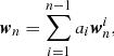
Methods. We explore three families of magnetic field configurations. First, a force-free helical magnetic field corresponding to a dynamically relaxed field in the rest frame of the jet. Second, a magnetic field with a co-axial cable structure arising from the Biermann-battery effect at the accretion disk. Third, a braided magnetic field that could be generated by turbulent motion at the accretion disk. We evaluate the intensity of synchrotron emission, the intrinsic polarization profile and the Faraday rotation measure arising from these fields. We assume that the jet consists of a relativistic spine where the radiation originates from and a sheath containing thermalised electrons responsible for the Faraday screening. We evaluate these values for a range of viewing angles and Lorentz factors. We account for Gaussian beaming that smooths the observed profile.
Results. Radio emission distributions from the jets with dominant large-scale helical fields show asymmetry across their width. The Faraday rotation asymmetry is the same for fields with opposing chirality (handedness). For jets which are tilted towards the observer the synchrotron emission and fractional polarization can distinguish the field’s chirality. When viewed either side-on or at a Blazar type angle only the fractional polarization can make this distinction. Further this distinction can only be made if the direction of the jet propagation velocity is known, along with the location of the jet’s origin. The complex structure of the braided field is found not to be observable due to a combination of line of sight integration and limited resolution of observation. This raises the possibility that, even if asymmetric radio emission signatures are present, the true structure of the field may still be obscure.
Key words: magnetic fields / relativistic processes / ISM: jets and outflows / methods: data analysis / radio continuum: general
© ESO 2019
1. Introduction
AGN are the most luminous long-lived sources in the Universe, outshining their host galaxies and persisting for millions of years (Fabian 1999). Their power can exceed 1046 erg s−1 and originates from a central engine consisting of a supermassive black hole and an accretion disc (Salpeter 1964; Zel’dovich 1964). While the gravitational energy released from the material accreted to the black hole is sufficient to match the energetics of the jet, the actual formation of the jet is a highly non-trivial process. Pure hydrodynamical models cannot explain jet launching. The role of a magnetic field in the vicinity of the black hole has been stressed from the very early works about these sources (Lynden-Bell 1969). The formation of the jet could be related to a dynamo action at the accretion disk which leads to the formation of two oppositely propagating magnetic beams (Lovelace 1976).
The magnetic field has also a central role in the Blandford-Znadjek mechanism that describes the extraction of energy from a Kerr black hole through a magnetic field that powers a jet (Blandford & Znajek 1977). Alternatively if the magnetic field is coupled to the accretion disc the energy can be extracted through the Blandford-Payne mechanism (Blandford & Payne 1982). These mechanisms do not depend on the polarity of the magnetic field with respect to the flow direction. If, on the other hand, the magnetic field originates from a cosmic battery phenomenon (Contopoulos & Kazanas 1998), then the polarity of the magnetic field will depend on the jet flow direction. In this model the electrons of the accretion disk experience a Poynting- Robertson drag, slowing them down with respect to the disk flow. This generates a net current and flux loops. Due to differential rotation, these loops open up, while accretion accumulates flux of one polarity at the inner part of the disk and the opposite polarity at the outer edge. This leads to the eventual formation of a toroidal magnetic field that corresponds to an electric current anti-parallel to the jet flow in the inner part of the jet, and parallel to the flow in the outer part (Contopoulos et al. 2006). The overall picture resembles that of a cosmic co-axial cable with electric current flowing towards the origin of the jet at the inner part of the cable and in the opposite direction in the outer part of the cable (Gabuzda et al. 2018).
A magnetic field anchored to an accretion disk that rotates rapidly might be twisted in similar manner, thus one might expect it to generate helical magnetic field (Spruit 2010). One assumption made in modelling this possibility is that the jet can be described by a close to ideal magnetohydrodynamical fluid with a magnetic field whose Lorentz force is the dominant driver of the field’s evolution (e.g., Königl & Choudhuri 1985). Following an argument of Taylor (1974), magnetic re-connection at sites where entanglement of the field lines is complex, and hence the local current is high, means that only large scale twisting induced by the rotation of the field will survive the field’s relaxation (the average magnetic helicity of the field is conserved). Under this assumption the system should relax to a force-free equilibrium, which, in the fluid frame where the electric field vanishes, takes the form
 (1)
(1)
with α a constant in space. This argument was applied to jets by Königl & Choudhuri (1985). Solutions of Eq. (1) in cylindrical geometry lead to configurations such as the reverse field pinch (Lundquist 1951) were used to interpret emission data in Clausen-Brown et al. (2011).
Since the possibility of turbulent motion in the accretion disc has long been considered viable (Stella & Rosner 1984; Subramanian et al. 1996; Balbus & Hawley 1998; Carballido et al. 2005; Lesur & Longaretti 2005) it seems sensible to consider the possibility that this motion could impart itself into the jet’s magnetic field, leading to more complex magnetic field configurations than a helical field. In such a system magnetic field lines anchored onto the accretion disk might experience extra local twist in addition to the global differential rotation. Even if the force free condition holds significantly complex structures can arise in Eq. (1) if α is allowed to vary in space (this has long been considered in Solar coronal modelling which relies on similar assumptions e.g., DeRosa et al. 2009; Su et al. 2009; Wiegelmann & Sakurai 2012). Moreover, the inclusion of the plasma thermal pressure leads to further modifications of the force-free equilibrium (Gourgouliatos et al. 2012). Attempting to simulate this possibility would be a complex task so we consider here a sensible first step to see if the possibility of significantly complex magnetic fields can be reconciled with observational data.
While the magnetic field is critical for the dynamics of the jet it is also the catalyst for the generation of the observed non-thermal emission. This comes through two main effects: synchrotron radio emission and Faraday rotation. Synchrotron radiation is produced when charged particles gyrate round magnetic field lines and experience acceleration. Because of this acceleration, these particles generate polarised radio waves (Rybicki & Lightman 1986). The intensity and polarisation of the synchrotron emission received by an observer depends on the population of relativistic electrons and the intensity of the magnetic field perpendicular to the line-of-sight vector, the vector originating from the observer to the source of radiation. Once polarised emission crosses a thermalised optically thin electron gas containing a magnetic field, the polarisation plane shifts due to Faraday rotation. The level of Faraday rotation is proportional to the integral of the magnetic field component along the line-of-sight, the thermal electron number density and the square of the wavelength of the radio emission. Thus, by taking observations at different wavelengths, one can measure the value of the rotation measure.
Therefore, the effects of the jet magnetic field can be indirectly probed through radio observations. This information depends on the line-of-sight integrated effect of the magnetic field and obviously information is lost due to the two dimensional projection of a three dimensional structure. In addition to the geometric effects, the highly relativistic nature of astrophysical jets, makes interpretation more complicated due to relativistic aberration and Doppler shifting. Because of these effects, the angle between the line-of-sight vector and the jet velocity changes and needs to be accounted for when observable properties are to be extracted. Finally there is the matter of the limited resolution due to the finite beam size of the radio telescope (Hovatta et al. 2012). This leads to the loss of the various emission features due to convolution of the actual signal with the radio beam (Clausen-Brown et al. 2011).
Extensive imaging surveys using very long base interferometry has permitted milliarcsecond resolution (Zensus 1997) radio-imaging of the central part of the AGN to sub-parsec scales (e.g., Walker et al. 2018). Such observations have revealed transverse asymmetries in the fractional polarisation and Faraday rotation measure implying that a large scale ordered magnetic field is present in the jet (Asada et al. 2002; Mahmud et al. 2013; Gabuzda et al. 2015; Motter & Gabuzda 2017). While the presence of the magnetic field in jets is indisputable, its exact structure is yet to be resolved (Hovatta et al. 2018).
In this paper we explore three main families of magnetic field configuration, extracting their observational properties. Two are based on fields that have previously been proposed to exist in relativistic jets, the reverse pinch field ascribed to the Taylor relaxation hypothesis (Königl & Choudhuri 1985; Clausen-Brown et al. 2011) and a representation of coaxial field of the type proposed in Contopoulos et al. (2009), Gabuzda et al. (2018). There is no analytical expression for the magnetic field for the battery/coaxial cable model, so we have proposed simple representation in order to compare its expected observations to those of the previously studied reverse-field pinch. The aim is to see if they could be distinguished. The third field is a braided field used in Pontin et al. (2011), Wilmot-Smith et al. (2010), Prior & Yeates (2016) as the initial configuration of a field which relaxes to a non-Taylor state (as discussed above). This last field is used in this note not as a realistic proposed model of the jet’s field, but as an indication of the variety structures which could explain radio observations. What is crucial here is that the size and strength of the braided field structure is such that it would significantly affect the evolution of a large scale magnetic field. This field, whilst complex is also significantly organised and large scale, thus differs from the class of disorganised fields used in Laing (1981).
In Sect. 2 we present a geometrical model of the observation of the jet and the specific models used for the jet’s magnetic field. We also discuss the appropriate relativistic transformations to produce synthetic images of the jets emission properties. In Sect. 3 we present the results of a survey of synthetic observational signals of the various magnetic field configurations, viewing angles and jet velocities. In Sect. 4 we consider some mathematical aspects of the loss of information due to the finite beam width which give some insight as to the type of emission structures which cannot be detected using this method. In Sect. 5 we compare our results to some observations and in Sect. 6 we conclude.
2. The toy jet radio emission model
2.1. Basic geometry
The model geometry is indicated in Fig. 1. We consider one arm of a jet whose origin coincides with the origin of a Cartesian coordinate system (x, y, z). An observer is placed at ( − do, 0, 0) and the axis of the jet, the direction of its bulk velocity (magnitude βc with c the speed of light) v lies in the y-z plane i.e. v = βc(−cosθj,0,sinθj), with θj = 0 meaning the jet is pointing towards the observer and θj = π pointing away. We assume the field is defined within a cylinder of radius 1 and height h.
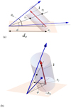 |
Fig. 1. Representations of the model geometry. In panel a we see the model as viewed along the y-axis. In panel b the same figure is seen from “over the shoulder” of the observer. The jet direction J is shown as a red arrow, the jet angle θj this makes with the x-axis is also shown. The distance do from the observer to the jet along the x axis is shown. The Blue arrow skimming the jet’s upper surface indicates the maximum angle subtended by the jet to the viewer θm. A black line, representing the direction of photon observation, pierces the cylinder surface at s1 and s2 subtends an angle θ < θm. The second blue arrow indicates the maximum (in magnitude) ϕ angle −ϕm subtended by the viewer and the jet’s side edge, as indicated in panel b. Also shown in panel b as a dotted line is the projection of the photon observation direction into the x-y plane and the angle ϕ which indicates its off-set from the jet’s central axis. |
2.2. Viewing angles
The direction of observation of the field is determined by the intersection with the jet of a set of lines l(s, θ, ϕ), with
 (2)
(2)
and consequently the direction of travel of the photons observed at the angle pair (θ, ϕ) is
 (3)
(3)
For each pair (θ, ϕ) the line l(s, θ, ϕ) will either intersect the jet cylinder twice or never, except where it skims the boundary. If the solution exists one obtains a pair s1(θ, ϕ) and s2(θ, ϕ) where the line enters and leaves the jet. Most of the emission quantities we calculate will be integrals over the line (l(s,θ,ϕ)|s∈[s1(θ,ϕ),s2(θ,ϕ)]). Thus we have a viewing domain 𝒟 = {(θ,ϕ)| θ∈[0,θm],ϕ∈[−ϕm,ϕm]}, with θm and ϕm the maximum viewing angles across the jet’s vertical extent and its width. When presenting the results we map this range of angles to the projected distances ϕd = sinϕ/sinϕmax and θd = sinθ/sinθmax with the normalisation for clarity i.e. θd = 0.5 is the viewing angle at half of the maximum vertical viewing extent.
For the calculations in this paper the ratio do/h will typically be large so the actual range of viewing angles arccos(n(θ, ϕ)⋅v) does not differ too much from those of the value of θj (allowing for the fact that they will be transformed due to relativistic aberration).
We now develop the models for the various radio emissions we simulate. The following largely follows the models described in Lyutikov et al. (2003, 2005); Clausen-Brown et al. (2011).
2.3. Stokes parameters and linear polarization
We calculate the following Stokes parameters
 (4)
(4)
where a prime indicates the quantity is expressed in the jet rest frame, here the integration is in the observer frame. The constant p is the electron index. The electron index depends on the process that has accelerated the electron population (Pacholczyk 1970; Drury 1983), we choose a value 1.5 in this text, changing this value within a reasonable range (1.5 < p < 3) does not significantly affect the results. All integrals are along the line of sight l(s, θ, ϕ). Since we are only interested in the qualitative comparison of distributions of these quantities the precise values of C1, C2 are not critical. The fields B will generally be specified in the jet frame (B′). The jet frame observation direction n′ is the aberration corrected (unit vector) direction along which the field is viewed, with
 (5)
(5)
(see e.g., Lyutikov et al. 2003). The function D = 1/γ(1 − v ⋅ n) is the Doppler boosting factor, where γ is the Lorentz factor (1 − β2)1/2. We introduce unit vector l normal to the plane containing the observation direction n and the reference direction in the plane of the sky, this will be the normalisation of  in our case (with
  a unit vector in the direction of v), then
 (6)
(6)
Assuming ideal MHD and following steps in Appendix C of Lyutikov et al. (2005) we find
![Mathematical equation: $$ \begin{aligned} \hat{\boldsymbol{e}}&= \frac{{\boldsymbol{n}}\times {\boldsymbol{q}}}{\sqrt{q^2-({\boldsymbol{n}}\cdot {\boldsymbol{q}})^2}}\quad {\boldsymbol{q}}=\hat{\boldsymbol{B}}+ {\boldsymbol{n}}\times ({\boldsymbol{v}}\times \hat{\boldsymbol{B}}),\\ \nonumber \hat{\boldsymbol{B}}&= \frac{1}{\sqrt{1-(\hat{\boldsymbol{B}}^\prime \cdot {\boldsymbol{v}})^2}}\left[\hat{\boldsymbol{B}}^\prime - \frac{\gamma }{1+\gamma }\hat{\boldsymbol{B}}^\prime \cdot {\boldsymbol{v}}\right], \end{aligned} $$](/articles/aa/full_html/2019/02/aa34469-18/aa34469-18-eq9.gif) (7)
(7)
where  is the unit vector field of B.
Using these Faraday variables we can calculate the fractional polarisation F as
 (8)
(8)
2.4. Faraday rotation
Following Clausen-Brown et al. (2011) the Faraday rotation R is
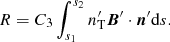 (9)
(9)
Where  is the (jet frame) thermal density of electrons. In this note we follow arguments given in Clausen-Brown et al. (2011) that the central core of the jet is responsible for synchrotron emission, but observational evidence indicates the Faraday screen responsible for the rotation is not co-spatial with this region. They propose a density for which the thermal electron density increases radially towards the edge of the jet, if ρ is the radial coordinate of the jet then the proposal is that
 (10)
(10)
where ρ is the radial distance form the jet’s central axis and k1 is chosen to fit the normalization of our tube (its radius is 1, which is not the case in Clausen-Brown et al. 2011). This is partly based on the choice of field in Clausen-Brown et al. (2011), a reverse pinch whose jet axis field reverses direction at ρ/k1 = 1.
2.5. The fields
In what follows we represent the field in cylindrical coordinates. In practice the field is then rotated to align with the axis of the jet.
2.5.1. The reverse field pinch Br
This is the field used in Clausen-Brown et al. (2011) and is used as a reference in this study. It can be written as
 (11)
(11)
with k2 = 3.8312, such that J1(k2)=0 and the field’s rotation vanishes on the boundary. To match the Faraday cage used in Clausen-Brown et al. (2011; i.e., Eq. (10)) we set k1 = 0.62761. This field has a uniformly right handed rotational component, but the sign of the field’s vertical component reverses at ρk1 = 1.
Calculations for the intensity I and Faraday rotation R for Eq. (11) for a slice of fixed θ values θd = 0.5 and ϕd ∈ [ − 1, 1] are shown in Fig. 2. These are calculated γ = 10 and jet angles θ which are similar to those used in Clausen-Brown et al. (2011). They have the same basic shape as those of, respectively, Figs. 2 and 4b of Clausen-Brown et al. (2011), except that the plots are antisymmetric about the y-axis (their ϕ observational behaviour is reversed). The reason for this is that the effect of viewing the jet from a significant distance in our model means we view it at an effective viewing angle in the form n = (−sin(ξ),0,cos(ξ)), where ξ is small. This contrasts to n = (sin(ξ),0,cos(ξ)) (as would have been used in Clausen-Brown et al. 2011) which would be more akin to an arm of a jet which is rotated from a negative direction rather than a positive. So in our choice of the orientation of the jet’s helical field, the line-of-sight component at ϕm is opposite to that of Clausen-Brown et al. (2011). The significant asymmetry results from the fact that for a helical geometry tilting the jet towards the observer will mean on one side of the field will appear close to normal to the observer, whilst the other side will appear close to parallel. This leads to a relative boosting of the signals either side of the central viewing direction. What is interesting here is the observation that, for a given field chirality (handedness), this asymmetry depends which arm of the jet is pointing toward the observer as well as the field chirality. We stress that the handedness would not necessarily be obvious unless the jet’s origin can be determined by observations, this is necessary to determine whether the photon propagation vector is n = (sin(ξ),0,cos(ξ)), or n = (−sin(ξ),0,cos(ξ)). Because of this, the choice of the slice along which the observational quantities are measured needs to be perpendicular to the jet direction and the location of jet’s origin needs to be taken into account. These can be easily determined for a radio galaxy jet seen side-on. However, in blazar observations appearing as circular intensity contours the jet’s direction needs to be determined by combining further high resolution and time evolution observations (Gabuzda et al. 2018; Lister et al. 2018).
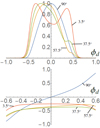 |
Fig. 2. Example I (panel a) and R (panel b) signatures for θd = 0.5 at jet angles θj = π/2, π/2 − π/16, π/2 − 2π/16 and π/16, which correspond to aberration corrected viewing angles of respectively 90°, 90 ° ,57.5 ° ,37.5 ° ,3.5°. |
2.5.2. The co-axial cable Bc
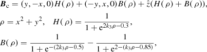
This is a representation of the coaxial-cable model (alternatively the battery model), proposed in Contopoulos et al. (2006), Gabuzda et al. (2018) as a field structure based on the observation of Faraday rotation profiles. In this note we represent it mathematically as
 (12)
(12)
If k3 is significant (we use k3 = 30 in this study) then the function H has roughly the shape of a smoothed Heaviside function (see Fig. 3a) whose value is 1 at zero, and the function B( ρ) creates a smooth bump whose peak value (between 0.6 and 0.8) is 1. The first two components of Bc are then twisted fields with opposing chirality (see Fig. 3b), they are chosen such that the current (approximately proportional to the curl of B) is negative at the field’s centre and positive near its edge. In this case it has a left-handed rotation on ρ ∈ [0, 0.4] and a right-handed rotation on ρ ∈ [0.4, 0.9]. The third component, which controls the z component of the field is negative on ρ ∈ [0, 0.4] and negative on ρ ∈ [0.4, 0.9]. The (helical) handedness of the field is opposite in the core and the sheath in comparison to the reverse-field pinch where the poloidal field changes sign but the toroidal does not.
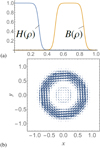 |
Fig. 3. Representations of the co-axial cable field Bc. Panel a: functions H( ρ) and B( ρ) used to define spatially distinct co-axial twists. Panel b: in plane representation of the vector fields showing the two sheaths of opposing twist. |
A specific mathematical form for this coaxial cable/battery model is not given. The form we chose here, with non-overlapping and largely uniform twisting domains contrasts with that of the reverse pinch whose two regions of current blend smoothly into one another. One consequence of this would be the existence of significant thin sheets of current between the two twists. This is by comparison the far more equally distributed current in the reverse pinch field, cf. a an b of Fig. 4. In principle we expect the coaxial cable field to obtain some dynamical state within the jet, which could give it a smoother profile, and we use the above mathematical expression as a framework to explore its effect on the observations.
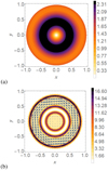 |
Fig. 4. Contour plots of the magnitude of the curl ∇ × B (a proxy for the current) in the field Br (panel a) and the coaxial cable Bc (panel b). The field Bc is overlayed on panel b. The maximum current in Bc is roughly an order of magnitude larger than in Br which occurs in think layers at the edges of the two twisting domains. |
2.5.3. A braided field B
This field has been used as an initial condition in numerous simulations in a non-relativistic MHD context Pontin et al. (2011), Wilmot-Smith et al. (2010), Prior & Yeates (2016). The field is composed of exponential twist units Bt(b0, k, a, l, xc, yc, zc) given by
 (13)
(13)
where the parameter b0 determines the strength of the field, a the horizontal width of the twist zones, l their vertical extent and k the handedness of the twist (k = 1 is right handed). The centre of rotation is (xc, yc, zc). The braided field is then defined as a superposition of n pairs of positive and negative twists and a uniform vertical background field
 (14)
(14)
where, d is the offset from the jet’s axis, and sd is the vertical spacing between consecutive twists (of the same sign). An example is shown in Fig. 5. In this study the values we use are  , l = 2/48, ds = 1/3, b0 = 1, d = 1/5, these values are those used in Pontin et al. (2011), Wilmot-Smith et al. (2010), Prior & Yeates (2016) scaled proportionally to a domain of unit width. This field has significantly complex field line entanglement (caused by the staggered opposing twist structure) and its evolution leads to a diffuse current structure of small but significant current sheets. It can be shown to relax to a force-free state which is not a Taylor state (e.g., Wilmot-Smith et al. 2010). In a solar context it might be imagined to be produced either by a series of convective cells or entanglement due to complex mixing motion at its foot points. Here we simply use it as a field whose structure is significantly different form the twisted distributions, but whose complex structure is on a similar order of magnitude to the resolution of the observation (a fact we demonstrate in what follows).
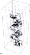 |
Fig. 5. A visualisation of the braided field used in this study. Units of (exponentially decaying) twist are arranged to overlap. The vertical background field is also shown. |
3. Results
Here, we explore the observational signatures varying the magnetic field structure, viewing angle and Lorentz factor. We have used two Lorentz factors γ = 10 for the highly relativistic case and γ = 2 for the mildly relativistic. We consider viewing angles between π/2 (edge on), π/3 (tilted) and π/30 (Blazar). In the highly relativistic case aberration effects mean the tilted field is viewed at an angle closer to 28°. We perform our calculations assuming the ratio of the observer distance do, to the jet height is 2 × 10⁵, which is equivalent roughly to a jet of 1 arc second extent if seen side-on. We did experiment with varying this ratio, but unless it is unrealistically small there is little qualitative effect in comparison to the results reported here. Thus, our results could be re-scaled for jets of arbitrary angular extent. We consider a jet of cylindrical shape and symmetry, where its height to radius ratio is 10.
We create synthetic images of both the Faraday rotation R and the fractional polarization F, in both cases these are over-layed on contours of the radio intensity I.
Using the procedure detailed in Sect. 2, we calculate the distributions on a grid of 50 × 50. To mimic the effect of beam convolution, we apply a Gaussian matrix of standard deviation 0.1 along the x-direction and 0.2 along the y direction (which represents twice the scaled distance). These standard deviations are the same as used in Clausen-Brown et al. (2011). We refer to these smoothed quantities as Fs, Is and Rs in what follows. Typically the beam size will be larger than this (e.g., Asada et al. 2002; Hovatta et al. 2012; Gabuzda et al. 2015), we ran calculations with larger beam sizes and found no difference from the results presented (save a rescaling of the pattern dimensions), so in some sense these results indicate the (current) best case scenario for radio observation.
For the sake of clarity we normalise the quantities R, Rs, I and Is between [ − 1, 1], the dimensionless fractional polarization results are not normalised.
3.1. Reverse pinch vs Coaxial cable
The Faraday rotation profiles of both Br and Bc in the highly relativistic case γ = 10 (the value used in Clausen-Brown et al. 2011) can be seen for viewing angle θj = π/3 in Fig. 6a. The “side-on” case θj = π/2 (no relativistic aberration) is shown in Fig. 7a. In both cases there is an asymmetry present in Rs, it is somewhat more pronounced in the side-on case. What is perhaps surprising is that the gradient of the curves is the same in both cases. Specific 1D slices are taken at θd = 0.5 in both the tilted and side-on cases which illustrate this, these plots are shown in Fig. 9. The coaxial gradients are more pronounced, as one might expect due to the fact that its rotation does not decay smoothly like the reverse pinch field, rather it is mostly constant as a function of radius (except over a small range). The Blazar case θj = π/30 is shown in Fig. 8. In all three cases there is a minimal asymmetry along the ϕd direction a fact made clear in the 1D slices are taken at θd = 0.5 (Fig. 9c). Of course if the slice were chosen for only part of this domain (say ϕd ∈ [0, 0.6]) then one would see a gradient. This would also be true if the slice were taken at an angle rather than for fixed θd.
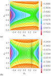 |
Fig. 6. Contour plots of the intensity in black and the Faraday rotation profiles shown in colour of the two large scale helical fields for highly relativistic jets γ = 10 with viewing angle θj = π/3. Panel a: Rs, for the field Br, panel b: Rs, for the field Bc. The horizontal and vertical axes are scaled so that they they cover the extend of ϕd and θd as described in Sect. 2.1. |
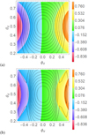 |
Fig. 7. Contour plots of the intensity in black and the Faraday rotation profiles shown in colour, of the two large scale helical fields for highly relativistic jets γ = 10 with viewing angle θj = π/2. Panel a: Rs, for the field Br, panel b: Rs, for the field Bc. |
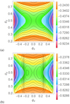 |
Fig. 8. Contour plots of the intensity in black and the Faraday rotation profiles shown in colour, of the two large scale helical fields for highly relativistic jets γ = 10 with viewing angle θj = π/30. Panel a: Rs, for the field Br, panel b: Rs, for the field Bc. |
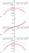 |
Fig. 9. Slices of the (smoothed) Faraday rotation Fs at θd = 0.5 for the fields Br (dashed) and Bc (solid). Panel a: tilted case. Panel b: side on case. Panel c: Blazar case. |
As expected the contours of Is do show opposing asymmetry for the two fields in the tilted case (see Clausen-Brown et al. 2011), see Fig. 10a as well as the less obvious the Blazar case (Fig. 10c). The Blazar case has two peaks close to the centre of the observer’s viewpoint, this is also clear in Fig. 8. It is interesting to observe a number of Blazar observations have this twin peak contour structure, whereas some don’t (see e.g., Gabuzda et al. 2018). The relatively sharp transition in twisting of the coaxial field leads to a slightly more interesting sub-structure in the contours of Is, as indicated in Figs. 10a and c. The side-on case, as expected shows no asymmetry for either field (Fig. 10b). So we can distinguish the two different field chiralities if the field is tilted, but we have to interrogate the Intensity profiles in that case. Further, as discussed in Sect. 2.5.1, we could only make this distinction if we know the position of the jet origin with respect to the observer and the jet’s tip. In the side on case it would appear from this information to be difficult to discriminate between globally twisted fields of two opposing chiralities.
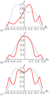 |
Fig. 10. Slices of the (smoothed) Synchrotron radiation Intensity Is at θd = 0.5 for the fields Br (dashed) and Bc (solid). Panel a: θj = π/3, panel b: θj = π/2 and panel c: θj = π/30. |
Slices of the fractional polarization Fs are shown in Fig. 11a for the tilted jet (θj = π/3) the side-on jet b and the Blazar jet c (we show the negative of these values for easy comparison to the results of Clausen-Brown et al. 2011). The side on and tilted case have clear asymmetry and the two chirality fields have opposing gradients, the Blazar case is symmetric for both fields (we also tried an angle π/16 which did show some asymmetry). Unlike for the intensity Is the Fs for side-on jets has the property of asymmetry. As with the intensity plots there is an additional structure in the coaxial cable where the exponential twisting transitions occur.
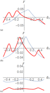 |
Fig. 11. Slices of the (smoothed) fractional polarization intensity −Fs at θd = 0.5 for the fields Br (dashed) and Bc (solid). Panel a: tilted field, panel b: side on field, panel c: Blazar. |
We now consider similar calculations in the weakly relativistic case γ = 2. We restrict to the tilted and Blazar cases as they affected by the value of γ. We see in Figs. 12 and 13 the story is largely similar with the Faraday rotation profiles still appearing as similar (although the gradients are more distinct) and the intensity distinguishing the field’s chirality. Finally the fractional polarisation Fs distribution is asymmetric with opposing gradients for the two fields (as in the highly relativistic case). The only difference from the highly relativistic case is that the fractional polarization slices do show asymmetry for the Blazar jet.
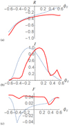 |
Fig. 12. A comparison of slices of Rs (panel a), Is (panel b) and Fs (panel c) for the helical fields Br (dashed) and Br in a tilted jet θj = π/3 with γ = 2. The slices are taken at θd = 0.5. |
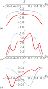 |
Fig. 13. A comparison of slices of Rs (panel a), Is (panel b) and Fs (panel c) for the helical fields Br (dashed) and Br in a Blazar jet θj = π/30 with γ = 2. The slices are taken at θd = 0.5. |
3.2. Braiding
The Faraday rotation profiles of Bb in the highly relativistic case γ = 10 can be seen for a viewing angle θ = π/3 in Fig. 14. We also plot the pre-Gaussian smoothed distributions I and R to highlight the loss of information which occurs due to the low resolution of observations. The Faraday rotation profiles are (almost) symmetric (see Fig. 16a). A similar story is true of the Blazar case, Fig. 15 where the pre-smoothed Faraday rotation profiles show no asymmetry along the ϕd direction (although there is some sense of asymmetry along the θd direction, this is lost upon applying the Gaussian filter. We note in this case the Faraday profiles are remarkably similar to those of the reverse pinch (Bessel) field shown in Fig. 8a.
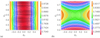 |
Fig. 14. Faraday rotation profiles for the braided field Bb at the tilted viewing angle θj = π/3. Panel a: R, panel b: Rs. |
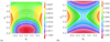 |
Fig. 15. Faraday rotation profiles for the braided field Bb at the tilted viewing angle θj = π/30. Panel a: R, panel b: Rs. |
In both the tilted and Blazar case the complexity of field is present in the pre-smoothed contours of I (Figs. 14a and 15a). Much of this information is lost upon applying the Gaussian filter and replaced with a set of slightly asymmetric contours in the tilted case Fig. 14b, as highlighted in Fig. 16b. In the Blazar case there is perfectly asymmetric bi-modal peaked distribution (see Figs. 17a and 17b). Similarly, as indicated in Figs. 16c and 17c the fractional polarization c is essentially symmetric for both viewing angles (actually symmetric in the blazar case). We emphasize that the Blazar Intensity distribution of this braided field is qualitatively the same as that of the reverse pinch field (cf. Figs. 17b and 10c), however, the fractional polarization distribution is symmetric where for the reverse pinch field is asymmetric (cf. Figs. 17c and 11c).
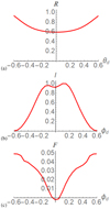 |
Fig. 16. Slices of the distributions Rs (panel a) and Is (panel b) and Fs (panel c) at θd = 0.5 for the braided field Bb at the tilted viewing angle. |
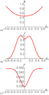 |
Fig. 17. Slices of the distributions Rs (panel a) and Is (panel b) and Fs (panel c) at θd = 0.5 for the braided field Bb at the Blazar viewing angle. |
The same distributions are shown for the side-on case θj = π/2 in Fig. 18. Pre-smoothing (Fig. 18a) the braided structure is clear in the Faraday rotation profiles (unlike in the tilted case shown in Fig. 16a), which actually show a series of alternating gradients with height. The intensity contours indicate the spatial variance of the field, but the varying offset twist structure is lost due to line of sight averaging. However, almost all of this information is lost in the smoothing process as shown in Fig. 18b, which shows gradients in neither Is or Rs. We do not show the fractional polarization profile as it is qualitatively similar to the tilted case (symmetric). Further we do not report on the results for γ = 2 as they tell a qualitatively similar story.
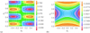 |
Fig. 18. Faraday rotation profiles for the braided field Bb at the side-on viewing angle θj = π/2. Panel a: R, panel b: Rs. |
The main conclusion we take here is that radio observations can hide significant complexity in magnetic field structure as a consequence of both line-of sight averaging and the limited spatial resolution of observations. It is interesting to note that in the side on case it is the Gaussian convolution which removes the Faraday rotation structure, whilst, for the tilted and Blazar jet case much of that structure is already lost due to the line of sight averaging. We will revisit this issue in Sect. 4.
3.3. Asymmetry and braiding
For non-Blazar type observations Faraday rotation data is sufficient to distinguish the braided field from the large scale helical fields which show asymmetry in their profiles (although as discussed above, the Faraday rotation struggles to make the distinction between braided and straight fields). For blazar fields we can still discriminate between the two fields types, but only with the fractional polarization data (and even then this depends on the value of γ). One might then ask what would happen if the jet field had a mixture of the two field types? In Fig. 19 we see the Faraday rotation profiles Rs for the composite field Bc + Bb (note the fields are of a same order of magnitude at their maximum). This covers both side-on and blazar jets. The Faraday rotation profiles consistently shows the asymmetry of the twisted field. In a (γ = 2, θj = π/3) we see the asymmetry of profile of I. As for the potential for Blazar distinction, the fractional polarization distribution is qualitatively similar to the coaxial cable case (an example is shown in Fig. 20), in the sense they both have a similar asymmetry.
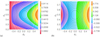 |
Fig. 19. Distributions of the (smoothed) Faraday rotation profiles Rs for the field Bc + Bb, in the case of a tilted jet with γ = 2 (panel a), a side-on jet with γ = 10 (panel b). |
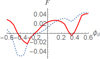 |
Fig. 20. Slices of the fractional polarisation at θd = 0.5 for the coaxial cable Bc (dashed) and the mixed field Bc + Bb, both for a weakly relativistic (γ = 2) blazar field θ = π/30. |
The crucial point here is that one could easily observe the kind of gradients expected of a large scale helical field but miss the signature of an additional component (of significant scale) which would lead to a far more complex jet magnetic field topology.
4. Types of structure loss
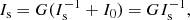
As discussed above there are several sources of information loss when synthetic observations are produced. One in particular takes simple form. The equation for converting a (discretely sampled) distribution I, F or R, i.e. a matrix (here we assume it is an n-by n matrix) into the observable (matrix) distributions Is, Ls and Rs, takes the form (e.g., for I)
 (15)
(15)
where G is a Gaussian matrix.
Mathematically the simplification of Is occurs due to the singular nature of the matrix G. Thus we could write this equation in the form
 (16)
(16)
where the matrix I0 is the part of he signal I which is in the kernel of G (GI0 = 0), the information which is lost, and  the part which is required to produce the observed signal (it can uniquely be determined by inversion (e.g., Horn & Johnson 1990). In short matricies I0 represent the distributions which are lost due to the finite beam width of the observational instrument. We have already seen in the previous section that braided patterns are, if not completely lost, significantly simplified by this transformation. Shortly we will show that the set of “lost” patterns which belong to I0 include striped and “spotted” such as shown in Fig. 21. But first we discuss the potential implications of this fact.
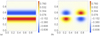 |
Fig. 21. Examples of the observationally lost distributions I0. Panel a: striped pattern, which could represent a gradient in the field. Panel b: pattern similar to that given in the Faraday rotation profiles of the braided field Bb. |
4.1. Balanced annulment and net zero-helicity fields
As indicated in Fig. 21 the distributions which are not observable tend to have an equal amount of positive and negative density. This occurs for the braided field Bb which has a balanced amount of both positive and negative twisting. It can be shown (e.g, Russell et al. 2015) that this means its magnetic helicity, a quantity which measures the average entanglement of the magnetic field lines (Prior & Yeates 2014), is zero, even though it has a complex entanglement. In ideal or close to ideal Magnetohydrodynamics the magnetic helicity is conserved, hence the braided field through its evolution maintains an equal balance of twisting (Russell et al. 2015). Thus in an evolution of a (close to) ideal plasma, if complex structure is created (this could be on top of a net helicity field like a helical field), we should expect it to be balanced (in terms of its twisting structure). The results of this paper indicate this would produce emissive signatures for which the net zero helicity field structure will either be annulled or at the least significantly masked.
4.2. Characterising the lost information I0 mathematically
We can get a useful idea of some of the potential structures of the observationally lost matrices I0. The vector space of the matrix I0 is very large as the Gaussian matrix only has one degree of freedom, along the diagonal (i.e. the radial direction). A productive approach to describing this space is to use the singular decomposition form of the matrix G (Horn & Johnson 1990), which takes the form
 (17)
(17)
where M is a diagonal matrix (the singular equivalent of the eigenvalue matrix) and both V and U are unitary matrices. In this case all the matrices are real and M has only one non-zero entry (the first), which represents the above mentioned radial degree of freedom. Thus the matrix MV* has non zero entries only in the first row. Let us call this row (vector) w and assume it is n-dimensional. A plot of the coefficients of w is shown in Fig. 22, (we have scaled the x-axis between [0, 1] since this vector acts on columns of I0, which represent the θd direction). Note it takes the shape of a slice across a Gaussian, thus represents the above discussed radial degree of freedom. So we can construct a matrix I0 whose columns are n-dimensional and which are normal to w, we label such vectors wn; they are drawn from an n − 1 dimensional subspace. One way to make a simple basis for such vectors is to define vectors in the form
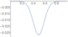 |
Fig. 22. Depiction of the “geometry” vector w. |
 (18)
(18)
i.e. for a given i we swap the ith and (i + 1)th entry of w and make the ith entry of the new vector the negative of what is was, then make all other entries 0. Thus we can write
 (19)
(19)
for some set of real coefficients  . For example if we chose all coefficients to be equal (ai = C) then the annulling vector wn has the geometry of the derivative of w (see Fig. 23a). Assuming this is the same for each column of I0 gives an ignored distribution in the form of a vertically asymmetric gradient (as shown in Fig. 21b). The symmetry of the Gaussian matrix means the same would be true of vertical stripes. But vertical stripes in this context would mean a gradient similar to that observed for the Faraday rotation (the decay outside the centre of the curve would result from decaying synchrotron emission outside of some jet core. The fact that in practice we don’t see the loss of such gradients is because the helical structure is of a scale larger than the size of the observation beam.
If we instead formed a matrix whose columns took the form shown in Fig. 23a, but whose coefficient values C varied across the columns (the θd direction) like a pair of Gaussian’s
 (20)
(20)
then we obtain a lost distribution very similar to the type expected for both I and R of the braided field, as shown in Fig. 21b. Of course in practice we saw the braided field has some measurable effect on the smooth distributions, this is because they were not always quite on the scale required to be fully annuled. The point here is that distributions which are asymmetric with respect to either the central θd or ϕd axes of the jet can be either lost or severely diluted as long as they are of a similar order of magnitude to the beam size. This might, for example make it hard to expect to detect a reverse gradient of the coaxial cable, as proposed by Gabuzda et al. (2018).
5. Discussion
Following the analysis in Sects. 3 and 4 we compare the conclusions of our exploration of magnetic field profiles with relativistic jet observations. As we have studied generic and simplified models our comparison will be qualitative rather than quantitative.
5.1. 3C 273
First, we consider 3C 273, a relativistic jet whose viewing angle is small < 16° (Abraham et al. 1996; Jorstad et al. 2017; Liodakis et al. 2018) and is believed to belong to the Blazar class. Milliarcsecond radio observations demonstrate a clear variation of the Faraday rotation measure across the jet (Asada et al. 2002), see Fig. 24. In this system the jet propagation direction is easily identifiable, (shown with a red arrow), and the section along which the rotation measured is perpendicular to this direction. Based on the various models we have explored, one can see this type of profile showing a gradient on a slice across the jet axis as in the helical or coaxial cable models (i.e. Fig. 7). Furthermore, this profile shows a counter-clockwise increase, thus if it is due to a coaxial cable configuration, one would see the outer part of the jet. We also note that this is consistent with a helical field with positive-handeness.
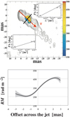 |
Fig. 24. Top panel: contours of radio emission of 3C 273 (black solid lines), with Faraday Rotation measure shown in colour. The jet propagation direction is shown with a red arrow. Bottom panel: Faraday Rotation measure along the black line, showing its transverse variation. Both figures reproduced by Asada et al. (2002). |
5.2. Blazar 0552+398
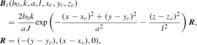
Next, let us consider the blazar source 0552+398 where the line of sight vector is almost parallel to the jet propagation direction (Gabuzda et al. 2018). In this case the sky-projected jet propagation velocity is not as clearly identifiable as in 3C 273, however in combination with data from Lister et al. (2018), a propagation direction as shown in the red arrow of Fig. 25 is favoured. In this case, one can attribute the rotation measure of this observation either to the inner part of a coaxial cable configuration, as its Faraday Rotation measure increases in the clockwise direction, or to a helical field with negative-handeness.
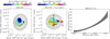 |
Fig. 25. Radio emission contours (shown in black) and Faraday rotation measure of 0552+398, shown in colour. The left panel is with an elliptical beam (shown at bottom left), the middle panel with a circular beam and the Faraday Rotation measure is shown in the right panel. The projected velocity on the plane of the sky is shown with a red arrow at the middle panel and the slice along which the Faraday Rotation is measures is plotted as a black line in the middle panel. Figure reproduced by Gabuzda et al. (2018). |
We note here, that as pointed in Clausen-Brown et al. (2011), the opening angle of blazar jets is comparable with the viewing angle, thus the simplified approximation of cylindrical jets reaches its limitations.
5.3. What could be missing?
These conclusions should be tempered by the fact we have seen in the previous two sections that additional complex field structure would not necessarily be present in these observations. In particular we have seen that the addition of the braided field to a large scale helical field still yields the kind of gradients which are observed in these two cases. Although it is beyond the scope of this study, one would expect significantly different reconnective activity if this more complex field were present, this could be manifested in high energy emission a possibility considered in Blandford et al. (2017).
6. Conclusion
From our exploration of jet magnetic field structure, Lorentz factor and viewing angle we can extract the following conclusions:
-
It is possible that magnetic field structure whose spatial variation is at least of the order of magnitude to be hidden from the various optical observations of the jet, including the Synchrotron intensity, Faraday rotation and Linear polarization distributions. This is a consequence of the combination of the line of sight averaging and limited optical resolution.
-
If the position of the centre of the jet is not known as discussed in Sect. 2.5.1, then it will not be possible to discriminate between large scale left and right handed helical fields.
-
Even if this relative orientation is known the Faraday rotation profiles do not discriminate the opposing chirality coaxial cable and reverse pinch large scale helical field structures.
-
If the field is almost side-on only the fractional polarization profiles (of the measures we consider here) can discriminate the opposing chirality coaxial cable and reverse pinch large scale helical field structures.
-
Small islands of Synchrotron emission intensity contours could potentially indicate sharp changes in the magnetic field toroidal orientation.
Recent analysis of radio observations (Gabuzda et al. 2015, 2018) have provided an ensemble of 52 sources where Faraday rotation measure can measured. Except for 5, the other 47 do not have any short time-scale variability and as of this, they can be used to identify a large scale magnetic field. According to that work 33 out of 47 have a rotation measure implying an electric current moving in the opposite direction of the jet propagation implying a coaxial cable. In our exploration of jet geometry we found that the side-on case shows clear gradient in the Faraday rotation. On the other hand, the signatures of titled jets are rather sensitive to contribution from the edges of the jet. As this part of the jet also corresponds to lower intensity, there could be observational biases with the central part of the jet being clearly observable, but the edge, where the contribution of a toroidal field could be higher to be practically invisible.
Finally, we remark that the gradient of the observable quantities could also depend on the choice of the slice. For instance a slice which is not normal to the jet’s velocity could lead to a drastically different Faraday rotation jet profile. While the direction of the jet axis can be clearly identified in jets seen edge-on, a small deviation could have drastic implications in jets that are seen head-on and practically appear as concentric circles in observations.
Acknowledgments
The authors would like to thank Daniele Dorigoni for a productive discussion regarding the singular value decomposition. We also thank Denise Gabuzda for permission to use Fig. 3 from Gabuzda et al. (2018) and discussion on the choice of the slice along which the RM is measured, and Maxim Lyutikov for insightful comments.
References
- Abraham, Z., Carrara, E. A., Zensus, J. A., & Unwin, S. C. 1996, A&AS, 115, 543 [NASA ADS] [Google Scholar]
- Asada, K., Inoue, M., Uchida, Y., et al. 2002, PASJ, 54, L39 [NASA ADS] [Google Scholar]
- Balbus, S. A., & Hawley, J. F. 1998, Rev. Mod. Phys., 70, 1 [Google Scholar]
- Blandford, R. D., & Payne, D. G. 1982, MNRAS, 199, 883 [NASA ADS] [CrossRef] [Google Scholar]
- Blandford, R. D., & Znajek, R. L. 1977, MNRAS, 179, 433 [NASA ADS] [CrossRef] [Google Scholar]
- Blandford, R., Yuan, Y., Hoshino, M., & Sironi, L. 2017, Space Sci. Rev., 207, 291 [NASA ADS] [CrossRef] [Google Scholar]
- Carballido, A., Stone, J. M., & Pringle, J. E. 2005, MNRAS, 358, 1055 [NASA ADS] [CrossRef] [Google Scholar]
- Clausen-Brown, E., Lyutikov, M., & Kharb, P. 2011, MNRAS, 415, 2081 [NASA ADS] [CrossRef] [Google Scholar]
- Contopoulos, I., & Kazanas, D. 1998, ApJ, 508, 859 [NASA ADS] [CrossRef] [Google Scholar]
- Contopoulos, I., Kazanas, D., & Christodoulou, D. M. 2006, ApJ, 652, 1451 [NASA ADS] [CrossRef] [Google Scholar]
- Contopoulos, I., Christodoulou, D. M., Kazanas, D., & Gabuzda, D. C. 2009, ApJ, 702, L148 [NASA ADS] [CrossRef] [Google Scholar]
- DeRosa, M. L., Schrijver, C. J., Barnes, G., et al. 2009, AJ, 696, 1780 [Google Scholar]
- Drury, L. O. 1983, Rep. Prog. Phys., 46, 973 [NASA ADS] [CrossRef] [Google Scholar]
- Fabian, A. C. 1999, Proc. Nat. Acad. Sci., 96, 4749 [NASA ADS] [CrossRef] [Google Scholar]
- Gabuzda, D. C., Knuettel, S., & Reardon, B. 2015, MNRAS, 450, 2441 [NASA ADS] [CrossRef] [Google Scholar]
- Gabuzda, D. C., Nagle, M., & Roche, N. 2018, A&A, 612, A67 [NASA ADS] [CrossRef] [EDP Sciences] [Google Scholar]
- Gourgouliatos, K. N., Fendt, C., Clausen-Brown, E., & Lyutikov, M. 2012, MNRAS, 419, 3048 [NASA ADS] [CrossRef] [Google Scholar]
- Horn, R. A., & Johnson, C. R. 1990, Matrix Analysis (Chapter 3) (Cambridge University Press) [Google Scholar]
- Hovatta, T., Lister, M. L., Aller, M. F., et al. 2012, AJ, 144, 105 [NASA ADS] [CrossRef] [Google Scholar]
- Hovatta, T., O’Sullivan, S., Martí-Vidal, I., Savolainen, T., & Tchekhovskoy, A. 2018, ArXiv e-prints [arXiv:1803.09982] [Google Scholar]
- Jorstad, S. G., Marscher, A. P., Morozova, D. A., et al. 2017, AJ, 846, 98 [Google Scholar]
- Königl, A., & Choudhuri, A. R. 1985, AJ, 289, 173 [NASA ADS] [CrossRef] [Google Scholar]
- Laing, R. 1981, AJ, 248, 87 [Google Scholar]
- Lesur, G., & Longaretti, P.-Y. 2005, A&A, 444, 25 [NASA ADS] [CrossRef] [EDP Sciences] [Google Scholar]
- Liodakis, I., Hovatta, T., Huppenkothen, D., et al. 2018, AJ, 866, 137 [Google Scholar]
- Lister, M. L., Aller, M. F., Aller, H. D., et al. 2018, ApJS, 234, 12 [NASA ADS] [CrossRef] [Google Scholar]
- Lovelace, R. V. E. 1976, Nature, 262, 649 [NASA ADS] [CrossRef] [Google Scholar]
- Lundquist, S. 1951, Phys. Rev., 83, 307 [NASA ADS] [CrossRef] [Google Scholar]
- Lynden-Bell, D. 1969, Nature, 223, 690 [NASA ADS] [CrossRef] [Google Scholar]
- Lyutikov, M., Pariev, V., & Blandford, R. D. 2003, AJ, 597, 998 [Google Scholar]
- Lyutikov, M., Pariev, V. I., & Gabuzda, D. C. 2005, MNRAS, 360, 869 [NASA ADS] [CrossRef] [Google Scholar]
- Mahmud, M., Coughlan, C. P., Murphy, E., Gabuzda, D. C., & Hallahan, D. R. 2013, MNRAS, 431, 695 [NASA ADS] [CrossRef] [Google Scholar]
- Motter, J. C., & Gabuzda, D. C. 2017, MNRAS, 467, 2648 [NASA ADS] [CrossRef] [Google Scholar]
- Pacholczyk, A. G. 1970, Radio Astrophysics. Nonthermal Processes in Galactic and Extragalactic Sources (San Francisco: W. H. Freeman) [Google Scholar]
- Pontin, D., Wilmot-Smith, A., Hornig, G., & Galsgaard, K. 2011, A&A, 525, A57 [NASA ADS] [CrossRef] [EDP Sciences] [Google Scholar]
- Prior, C., & Yeates, A. 2014, AJ, 787, 100 [CrossRef] [Google Scholar]
- Prior, C., & Yeates, A. 2016, A&A, 591, A16 [NASA ADS] [CrossRef] [EDP Sciences] [Google Scholar]
- Russell, A. J., Yeates, A. R., Hornig, G., & Wilmot-Smith, A. L. 2015, Phys. Plasmas, 22, 032106 [NASA ADS] [CrossRef] [Google Scholar]
- Rybicki, G. B., & Lightman, A. P. 1986, Radiative Processes in Astrophysics (New Jersey: Wiley), 400 [Google Scholar]
- Salpeter, E. E. 1964, ApJ, 140, 796 [CrossRef] [Google Scholar]
- Spruit, H. C. 2010, in Lect. Notes Phys., ed. T. Belloni (Berlin: Springer Verlag), 794, 233 [Google Scholar]
- Stella, L., & Rosner, R. 1984, ApJ, 277, 312 [NASA ADS] [CrossRef] [Google Scholar]
- Su, Y., van Ballegooijen, A., Lites, B. W., et al. 2009, AJ, 691, 105 [NASA ADS] [CrossRef] [Google Scholar]
- Subramanian, P., Becker, P. A., & Kafatos, M. 1996, ApJ, 469, 784 [NASA ADS] [CrossRef] [Google Scholar]
- Taylor, J. B. 1974, Phys. Rev. Lett., 33, 1139 [NASA ADS] [CrossRef] [Google Scholar]
- Walker, R. C., Hardee, P. E., Davies, F. B., Ly, C., & Junor, W. 2018, ApJ, 855, 128 [NASA ADS] [CrossRef] [Google Scholar]
- Wiegelmann, T., & Sakurai, T. 2012, Sol. Phys., 9, 5 [Google Scholar]
- Wilmot-Smith, A., Pontin, D., & Hornig, G. 2010, A&A, 516, A5 [NASA ADS] [CrossRef] [EDP Sciences] [Google Scholar]
- Zel’dovich, Y. B. 1964, Sov. Phys. Dokl., 9, 195 [NASA ADS] [Google Scholar]
- Zensus, J. A. 1997, ARA&A, 35, 607 [NASA ADS] [CrossRef] [Google Scholar]
All Figures
|
Fig. 1. Representations of the model geometry. In panel a we see the model as viewed along the y-axis. In panel b the same figure is seen from “over the shoulder” of the observer. The jet direction J is shown as a red arrow, the jet angle θj this makes with the x-axis is also shown. The distance do from the observer to the jet along the x axis is shown. The Blue arrow skimming the jet’s upper surface indicates the maximum angle subtended by the jet to the viewer θm. A black line, representing the direction of photon observation, pierces the cylinder surface at s1 and s2 subtends an angle θ < θm. The second blue arrow indicates the maximum (in magnitude) ϕ angle −ϕm subtended by the viewer and the jet’s side edge, as indicated in panel b. Also shown in panel b as a dotted line is the projection of the photon observation direction into the x-y plane and the angle ϕ which indicates its off-set from the jet’s central axis. |
| In the text | |
|
Fig. 2. Example I (panel a) and R (panel b) signatures for θd = 0.5 at jet angles θj = π/2, π/2 − π/16, π/2 − 2π/16 and π/16, which correspond to aberration corrected viewing angles of respectively 90°, 90 ° ,57.5 ° ,37.5 ° ,3.5°. |
| In the text | |
|
Fig. 3. Representations of the co-axial cable field Bc. Panel a: functions H( ρ) and B( ρ) used to define spatially distinct co-axial twists. Panel b: in plane representation of the vector fields showing the two sheaths of opposing twist. |
| In the text | |
|
Fig. 4. Contour plots of the magnitude of the curl ∇ × B (a proxy for the current) in the field Br (panel a) and the coaxial cable Bc (panel b). The field Bc is overlayed on panel b. The maximum current in Bc is roughly an order of magnitude larger than in Br which occurs in think layers at the edges of the two twisting domains. |
| In the text | |
|
Fig. 5. A visualisation of the braided field used in this study. Units of (exponentially decaying) twist are arranged to overlap. The vertical background field is also shown. |
| In the text | |
|
Fig. 6. Contour plots of the intensity in black and the Faraday rotation profiles shown in colour of the two large scale helical fields for highly relativistic jets γ = 10 with viewing angle θj = π/3. Panel a: Rs, for the field Br, panel b: Rs, for the field Bc. The horizontal and vertical axes are scaled so that they they cover the extend of ϕd and θd as described in Sect. 2.1. |
| In the text | |
|
Fig. 7. Contour plots of the intensity in black and the Faraday rotation profiles shown in colour, of the two large scale helical fields for highly relativistic jets γ = 10 with viewing angle θj = π/2. Panel a: Rs, for the field Br, panel b: Rs, for the field Bc. |
| In the text | |
|
Fig. 8. Contour plots of the intensity in black and the Faraday rotation profiles shown in colour, of the two large scale helical fields for highly relativistic jets γ = 10 with viewing angle θj = π/30. Panel a: Rs, for the field Br, panel b: Rs, for the field Bc. |
| In the text | |
|
Fig. 9. Slices of the (smoothed) Faraday rotation Fs at θd = 0.5 for the fields Br (dashed) and Bc (solid). Panel a: tilted case. Panel b: side on case. Panel c: Blazar case. |
| In the text | |
|
Fig. 10. Slices of the (smoothed) Synchrotron radiation Intensity Is at θd = 0.5 for the fields Br (dashed) and Bc (solid). Panel a: θj = π/3, panel b: θj = π/2 and panel c: θj = π/30. |
| In the text | |
|
Fig. 11. Slices of the (smoothed) fractional polarization intensity −Fs at θd = 0.5 for the fields Br (dashed) and Bc (solid). Panel a: tilted field, panel b: side on field, panel c: Blazar. |
| In the text | |
|
Fig. 12. A comparison of slices of Rs (panel a), Is (panel b) and Fs (panel c) for the helical fields Br (dashed) and Br in a tilted jet θj = π/3 with γ = 2. The slices are taken at θd = 0.5. |
| In the text | |
|
Fig. 13. A comparison of slices of Rs (panel a), Is (panel b) and Fs (panel c) for the helical fields Br (dashed) and Br in a Blazar jet θj = π/30 with γ = 2. The slices are taken at θd = 0.5. |
| In the text | |
|
Fig. 14. Faraday rotation profiles for the braided field Bb at the tilted viewing angle θj = π/3. Panel a: R, panel b: Rs. |
| In the text | |
|
Fig. 15. Faraday rotation profiles for the braided field Bb at the tilted viewing angle θj = π/30. Panel a: R, panel b: Rs. |
| In the text | |
|
Fig. 16. Slices of the distributions Rs (panel a) and Is (panel b) and Fs (panel c) at θd = 0.5 for the braided field Bb at the tilted viewing angle. |
| In the text | |
|
Fig. 17. Slices of the distributions Rs (panel a) and Is (panel b) and Fs (panel c) at θd = 0.5 for the braided field Bb at the Blazar viewing angle. |
| In the text | |
|
Fig. 18. Faraday rotation profiles for the braided field Bb at the side-on viewing angle θj = π/2. Panel a: R, panel b: Rs. |
| In the text | |
|
Fig. 19. Distributions of the (smoothed) Faraday rotation profiles Rs for the field Bc + Bb, in the case of a tilted jet with γ = 2 (panel a), a side-on jet with γ = 10 (panel b). |
| In the text | |
|
Fig. 20. Slices of the fractional polarisation at θd = 0.5 for the coaxial cable Bc (dashed) and the mixed field Bc + Bb, both for a weakly relativistic (γ = 2) blazar field θ = π/30. |
| In the text | |
|
Fig. 21. Examples of the observationally lost distributions I0. Panel a: striped pattern, which could represent a gradient in the field. Panel b: pattern similar to that given in the Faraday rotation profiles of the braided field Bb. |
| In the text | |
|
Fig. 22. Depiction of the “geometry” vector w. |
| In the text | |
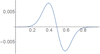 |
Fig. 23. Vector wn which is normal to the vector w depicted in Fig. 22. |
| In the text | |
|
Fig. 24. Top panel: contours of radio emission of 3C 273 (black solid lines), with Faraday Rotation measure shown in colour. The jet propagation direction is shown with a red arrow. Bottom panel: Faraday Rotation measure along the black line, showing its transverse variation. Both figures reproduced by Asada et al. (2002). |
| In the text | |
|
Fig. 25. Radio emission contours (shown in black) and Faraday rotation measure of 0552+398, shown in colour. The left panel is with an elliptical beam (shown at bottom left), the middle panel with a circular beam and the Faraday Rotation measure is shown in the right panel. The projected velocity on the plane of the sky is shown with a red arrow at the middle panel and the slice along which the Faraday Rotation is measures is plotted as a black line in the middle panel. Figure reproduced by Gabuzda et al. (2018). |
| In the text | |
Current usage metrics show cumulative count of Article Views (full-text article views including HTML views, PDF and ePub downloads, according to the available data) and Abstracts Views on Vision4Press platform.
Data correspond to usage on the plateform after 2015. The current usage metrics is available 48-96 hours after online publication and is updated daily on week days.
Initial download of the metrics may take a while.