| Issue |
A&A
Volume 691, November 2024
|
|
|---|---|---|
| Article Number | A14 | |
| Number of page(s) | 12 | |
| Section | Astrophysical processes | |
| DOI | https://doi.org/10.1051/0004-6361/202450978 | |
| Published online | 25 October 2024 | |
3D hybrid fluid-particle jet simulations and the importance of synchrotron radiative losses
1
Max-Planck-Institut für Radioastronomie, Auf dem Hügel 69, D-53121 Bonn, Germany
2
Theoretical Division, Los Alamos National Laboratory, Los Alamos, NM 87545, USA
3
Department of Physics and Astronomy, 108 Lewis Hall, University of Mississippi, Oxford MS 38677-1848, USA,
4
Julius-Maximilians-Universität Würzburg, Institut für Theoretische Physik und Astrophysik, Lehrstuhl für Astronomie, Emil-Fischer-Str. 31, D-97074 Würzburg, Germany
⋆ Corresponding author; This email address is being protected from spambots. You need JavaScript enabled to view it.
Received:
3
June
2024
Accepted:
1
September
2024
Abstract
Context. Relativistic jets in active galactic nuclei are known for their exceptional energy output, and imaging the synthetic synchrotron emission of numerical jet simulations is essential for a comparison with observed jet polarization emission.
Aims. Through the use of 3D hybrid fluid-particle jet simulations (with the PLUTO code), we overcome some of the commonly made assumptions in relativistic magnetohydrodynamic (RMHD) simulations by using non-thermal particle attributes to account for the resulting synchrotron radiation. Polarized radiative transfer and ray-tracing (via the RADMC-3D code) highlight the differences in total intensity maps when (i) the jet is simulated purely with the RMHD approach, (ii) a jet tracer is considered in the RMHD approach, and (iii) a hybrid fluid-particle approach is used. The resulting emission maps were compared to the example of the radio galaxy Centaurus A.
Methods. We applied the Lagrangian particle module implemented in the latest version of the PLUTO code. This new module contains a state-of-the-art algorithm for modeling diffusive shock acceleration and for accounting for radiative losses in RMHD jet simulations. The module implements the physical postulates missing in RMHD jet simulations by accounting for a cooled ambient medium and strengthening the central jet emission.
Results. We find a distinction between the innermost structure of the jet and the back-flowing material by mimicking the radio emission of the Seyfert II radio galaxy Centaurus A when considering an edge-brightened jet with an underlying purely toroidal magnetic field. We demonstrate the necessity of synchrotron cooling as well as the improvements gained when directly accounting for non-thermal synchrotron radiation via non-thermal particles.
Key words: magnetohydrodynamics (MHD) / radiation mechanisms: non-thermal / radiative transfer / relativistic processes / methods: numerical / galaxies: jets
© The Authors 2024
 Open Access article, published by EDP Sciences, under the terms of the Creative Commons Attribution License (https://creativecommons.org/licenses/by/4.0), which permits unrestricted use, distribution, and reproduction in any medium, provided the original work is properly cited.
This article is published in open access under the Subscribe to Open model.
Open Access funding provided by Max Planck Society.
1. Introduction
Active galactic nuclei (AGN) are supermassive black holes (SMBHs) that actively accrete matter, forming highly energetic, bright, compact objects in the centers of galaxies (Rees 1966). Approximately 10% of AGN are classified as radio-loud and are characterized by the presence of large-scale jets that remain collimated on up to kiloparsec scales (Homan et al. 2018). Radio-loud AGN encompass various classes, including radio galaxies and blazars, which differ in orientation with respect to our line of sight. While radio galaxies and blazars are believed to be the same intrinsic object, blazars show jets that are increasingly aligned to our line of sight (Urry & Padovani 1995).
The strength and orientation of magnetic fields in AGN can be determined through observations of power-law spectra and polarization signals in the radio regime. The strength of the intrinsic magnetic field is measured by assessing the apparent core shifts in optically thick synchrotron self-absorbed emission across various frequencies (see, e.g., Pushkarev et al. 2012). Lobanov (1998) calculated the magnetic field strengths of various radio sources by analyzing the core shift. The direction of the magnetic field is inferred from polarization measurements, particularly from the detection of both linearly and circularly polarized non-thermal synchrotron emission (Meisenheimer & Roeser 1986; Carilli et al. 1999; Heavens & Meisenheimer 1987; Brunetti et al. 2003).
Astrophysical jets associated with AGN are thought to carry helical magnetic field configurations near the central engine. However, the role of these helical fields on larger scales remains unclear (e.g., Gabuzda et al. 2008; Gabuzda 2018; Paraschos et al. 2021; Perucho et al. 2023; Kim et al. 2023). The synchrotron emission from these jets exhibits high degrees of linear polarization (LP; up to 60−70%; see, e.g., Rybicki & Lightman 1979; Todorov et al. 2023; Lister & Homan 2005; Park & Algaba 2022) and weaker circular polarization (CP; ∼1%). This polarized emission provides valuable insights into the intrinsic magnetic field structure (see, e.g., Tsunetoe et al. 2021). Numerical studies have shown that CP can be used to distinguish between poloidal and toroidal magnetic field morphologies within relativistic jets (Kramer & MacDonald 2021).
Multiwavelength observations, ranging from radio to high-energy gamma rays, offer valuable insights into the micro-physical processes occurring within AGN jets (EHT MWL Science Working Group 2021). These micro-physical processes (Pontin & Priest 2022) occur on physical scales several orders of magnitude smaller than the overall jet scale. Bridging the gap between these scales is a significant challenge for theoretical models of AGN jet emission.
Due to the inability to reproduce relativistic jets in laboratories, numerical simulations are the primary means of exploring the underlying physics (Bellan 2018). AGN jets can be effectively modeled as plasma since the Larmor radius of the jet particles is much smaller than the spatial scales of the system (Blandford & Rees 1974). Recently, a numerical algorithm has been developed within the PLUTO code to simulate multidimensional flow patterns, incorporating small-scale processes in a sub-grid manner (Mignone et al. 2007, 2019, 2023; Vaidya et al. 2018; Mandal et al. 2023; Melon Fuksman & Mignone 2019).
In general, synchrotron emission signatures from large-scale jets are obtained through time-dependent simulations and post-process radiative transfer. In relativistic hydrodynamic contexts, transfer functions between thermal and non-thermal plasma are implemented. In the case of relativistic magnetohydrodynamic (RMHD) calculations, the internal magnetic structure of the jet and the parameters of the energy distribution are used to compute synchrotron emission maps (Porth et al. 2011; Mizuno et al. 2015; Fromm et al. 2016; Kramer & MacDonald 2021).
To study the micro-physics of particle acceleration at shocks, hybrid implementations that combine particle and grid-based fluid descriptions have been developed, targeting different scales of interest. The particle-in-cell approach is often employed to understand particle acceleration at relativistic shocks, particularly at the scales of the electron gyro-radius. Hybrid MHD-particle-in-cell approaches enable the study of shock acceleration at slightly larger length scales, typically of the order of a few thousand proton gyro-radii. These approaches describe the interaction between collisionless cosmic ray particles and thermal plasma, capturing small-scale kinetic effects in magnetosphere simulations (e.g., Bai et al. 2015; van Marle et al. 2018; Mignone et al. 2018; Daldorff et al. 2014). Recently, Dubey et al. (2023), Sow Mondal et al. (2023), Nurisso et al. (2023), and Giri et al. (2022) explored the behavior of the observable emission from particles encountering various shock acceleration mechanisms within the jet stream in hybrid (R)MHD-particle simulations.
For relativistic hydrodynamic flows, the “painting” of non-thermal particle (NTP) populations onto thermal flows of plasma allows the study of non-thermal synchrotron emission from internal shocks in blazars (Mimica et al. 2009, 2012; Porth et al. 2011; Fromm et al. 2016). In these models, a simplifying assumption was made by setting a constant value for the power-law index that governs particle injection at shocks (N(E)∝E−s), with values such as s = 2.0 (de la Cita et al. 2016), s = 2.23 (Fromm et al. 2016), and s = 2.3 (Kramer & MacDonald 2021).
Fully Eulerian approaches to NTP transport have been successfully applied to numerical simulations over several decades (such as Kang et al. 1992). Additional methods have been developed by Vaidya et al. (2018) to overcome the aforementioned limitations and establish a state-of-the-art hybrid framework for particle transport. This framework aims to model high-energy non-thermal emission by including Lagrangian particles in large-scale 3D RMHD simulations. This is achieved by utilizing the magnetic field from the underlying RMHD simulation to calculate radiative losses, such as synchrotron cooling. The hybrid framework can be compared with observations by incorporating micro-physical aspects of spectral evolution based on local fluid conditions.
The emission from the accelerated charged particles within jets in various types of AGN, for example blazars and Seyfert II radio galaxies such as Centaurus A, is relativistically Doppler-beamed. Relativistic plasma and magnetic fields in AGN jets give rise to incoherent synchrotron emission components ranging in wavelength from the radio to the optical, the UV, or even X-rays, and can exhibit LP. The polarization parameters carry information about the jet’s physical conditions, including the magnetic field strength, topology, and particle density (Wardle et al. 1998).
This paper explores the effect that synchrotron cooling has on ray-traced images of a 3D RMHD jet with an orientation similar to Centaurus A. In particular, synchrotron cooling helps highlight the jetted structure relative to emission from the back-flowing cocoon of the jet (which has undergone synchrotron cooling). Previous models utilizing the PLUTO code have relied on numerical tracer values within the jet to artificially exclude the bow shock from emission calculations (as demonstrated in Kramer & MacDonald 2021). This paper demonstrates that incorporating particle physics is crucial for accurately modeling extragalactic sources (in the radio domain). We aim to mimic the characteristics of the nearby radio galaxy Centaurus A, and we discuss a qualitative comparison between our synthetic polarized emission maps and observations obtained from both the TANAMI program (Müller et al. 2014) and the Event Horizon Telescope Collaboration (EHTC), under the leadership of Janssen et al. (2021). A similar approach to mimic the radio galaxy 3C 84, using the methods described in this paper, is also successfully implemented in an accompanying paper (Paraschos et al. 2024).
This paper is organized as follows: In Sect. 2 we provide an introduction to the principles of the hybrid fluid-particle simulations used in the PLUTO code, with a focus on Lagrangian particles (i.e., macro-particles that represent numerous non-thermal micro-particles). We introduce the principles of particle physics within numerical jet simulations, namely the inclusion of radiative losses. We further focus on the numerical implementation of our relativistic jet simulations, along with the explanation of the post-process generation of a 3D grid, which is extrapolated from the NTP attributes. Section 3 outlines our applied method for calculating synthetic polarized synchrotron emission maps from particle simulations of jets via the ray-tracing code RADMC-3D. Section 4 compares our simulations to the nearby radio galaxy Centaurus A. Section 5 discusses the comparison between our numerical hybrid fluid-particle RMHD approach and observations of Centaurus A (Müller et al. 2014; Janssen et al. 2021). Finally, Sect. 6 provides our conclusions.
2. Lagrangian module
In recent years, researchers have recognized the importance of incorporating Lagrangian particles into (R)MHD simulations to gain deeper insights into the behavior of the jet plasma (Vaidya et al. 2018). Lagrangian particles are individual tracer elements that move with the thermal jet flow, providing valuable information about the fluid’s characteristics, such as its velocity, density, and magnetic field strength. By following the trajectories of these particles, we can track the transport and mixing of different plasma components. In particular, we examined the impact of magnetic fields on particle dynamics and studied various physical processes occurring within the jet. The use of Lagrangian particles in RMHD jet simulations allows us to perform a more detailed analysis of the complex phenomena taking place in these astrophysical systems. Hence, this approach enables the study of important processes, including particle acceleration mechanisms, the formation and propagation of shocks, and the effect of radiative losses within the relativistic jet.
2.1. Cosmic ray transport equation
The reduced cosmic ray transport equation for the relativistic case (Webb 1989) considers particle transport by both convection and diffusion, along with their evolution of momentum space. This includes energy changes due to adiabatic expansion or contraction, as well as caused by radiation processes. In particular, the time evolution of a NTP is governed by the following expression (Vaidya et al. 2018):
![Mathematical equation: $$ \begin{aligned} \frac{\mathrm{d}n_{\rm e}(E)}{\mathrm{d}\tau } + \frac{\partial }{\partial E}\left[\left(-\frac{E}{3}\nabla _\mu u^\mu + \dot{E}_l\right)n_{\rm e}(E)\right] = -n_{\rm e}(E) \nabla _\mu u^\mu , \end{aligned} $$](/articles/aa/full_html/2024/11/aa50978-24/aa50978-24-eq1.gif) (1)
(1)
where uμ is the bulk four-velocity, dτ is a time differential (related to the laboratory time), and γ is the electron Lorentz factor of the NTP. The ne(E) represents an electron (subscript e) energy distribution normalized to the particle number density. The particle energy distribution is initialized as a single power-law, with index s, in the form of ne(E)∝NeE−s. The terms within Eq. (1) in square brackets account for energy changes due to adiabatic expansion and radiative losses. This paper focuses on the second term (Ė1), which accounts explicitly for synchrotron cooling (Vaidya et al. 2018).
Equation (1) is solved in two steps. In the first step, the particle positions xp are evolved in time according to
 (2)
(2)
where vp is the particle velocity. The solution is performed using a second-order Runge-Kutta scheme that computes a predictor step followed by a corrector step (see, e.g., Mignone et al. 2007, 2019; Vaidya et al. 2016, 2018). In the second step, the energy change is accounted for by updating the energy distribution of the particle. Consequently, the energy term within Eq. (1) is solved. Section 2.2 provides a more detailed description of this solution considering radiative synchrotron losses in particular (Vaidya et al. 2018).
2.2. Synchrotron losses
To trace the synchrotron losses, the energy distribution of each macro-particle is continuously updated over time. Precisely, the code keeps track of the particle’s parameters at a given position on the Cartesian grid (by tracking the particle position according to Eq. (2)). The particle attributes are transferred in each numerical step and solved for the particle’s energy changes. The attributes are computed in the following fashion:
 (3)
(3)
In Eq. (3), the first term represents the energy loss resulting from adiabatic expansion, while the second term represents the combined energy loss from synchrotron radiation and inverse Comp- ton scattering off the cosmic microwave background1. The physical constants c1 and c2 are given as follows (Vaidya et al. 2018):
![Mathematical equation: $$ \begin{aligned} c_1 = \frac{\nabla _\mu u^\mu }{3}, \qquad c_2 = \frac{4\sigma _{\rm T}c\beta ^2}{3 m_e^2 c^4}\left[U_{B} + U_{\rm rad}\left(E_{\rm ph}\right)\right]. \end{aligned} $$](/articles/aa/full_html/2024/11/aa50978-24/aa50978-24-eq4.gif) (4)
(4)
The Thomson cross-section, denoted as σT, represents the scattering efficiency. The quantities UB and Urad correspond to the energy densities of the magnetic field and the radiation field, respectively. Eph represents the energy of the incident photon field from the cosmic microwave background (Vaidya et al. 2018).
2.3. Numerical implementation
The Lagrangian macro-particles represent ensembles of NTPs with finite energy distributions that are advected along fluid streamlines. The underlying flow is calculated by the RMHD module within PLUTO. Details on the principles of the RMHD module and physical scaling are provided in Kramer & MacDonald (2021), based on Mignone et al. (2007). The implementation of the magnetic field remains the same as in Kramer & MacDonald (2021). This paper focuses on a purely toroidal magnetic field prescription within a defined magnetization radius within to relativistic jet (i.e., σϕ = 1).
PLUTO stores the normalized energy distribution ne(E) of NTPs in logarithmically separated energy bins Emin ≤ E ≤ Emax (with E = Ebin in units of electron rest mass). We assumed an initial energy distribution at time step 0 (ne0(E)), of the NTPs that follows a global power-law distribution in energy, similar to Vaidya et al. (2018):
 (5)
(5)
We initialized the spectrum with a power-law index of s = 2. The spectral index, α, which is needed to calculate the resulting synchrotron emission, relates to the power-law index s via: α = (s − 1)/2. The power-law index and the spectral index are computed for each cell and, hence, are changing constantly throughout the computational domain (both spatially and temporally)2. nmicro denotes the initial number density of physical particles across energy bins:
 (6)
(6)
This formulation calculates the total energy in dimensionless units, that is, the area under the distribution per macro-particle in the energy spectra illustrated in Fig. 1. To account for physical values, nmicro is expressed in terms of density per atomic mass unit. We would like to emphasize that the expression in Eq. (6) changes for every Lagrangian particle, which is affected by the synchrotron cooling term in Eq. (1).
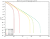 |
Fig. 1. Normalized spectral distribution in dimensionless grid units of a representative macro-particle. The corresponding Lagrangian particle is located in the jet’s spine just before entering the back-flow. The initial energy bins are chosen to be within 10 ≤ γ ≤ 107. The particle is injected onto the grid through the jet orifice at epoch 20 (each color represents a different simulation epoch). The radiative losses experienced by this NTP are visible as the particle’s energy distribution evolves (in time) from right to left. |
To calculate the synthetic non-thermal synchrotron emission from the Lagrangian particle attributes, we rewrote the power-law in terms of the electron Lorentz factor3, γ (E = γmec2). Similar to the study conducted in Kramer & MacDonald (2021), we set an initial bound between the lower energy cutoff γmin = 10 and the upper limit γmax = γmin ⋅ 106. Similar to Kramer & MacDonald (2021), we generated 3D grids of magnetic field strength B [Gauss], electron number densities nmicro [cm−3], low-energy power-law cutoffs γmin, and spectral indices α, from interpolation of our Lagrangian particle properties. These interpolated grids are then input into RADMC-3D. In order to compute the normalization constant, we further expressed the electron power-law distribution in terms of the electron Lorentz factor, γ:  for γmin ≤ γ ≤ γmax. Together with the continuous equivalent of Eq. (5), we arrive at the normalization constant
 (7)
(7)
The particle attributes, such as ne(γ), were evolved during the simulation. In a post-process step, we estimated the normalization constant, Ne, from the lower energy cutoff,γmin(≡Emin), and the power-law index, s, between two neighboring energy bins at a specific electron energy, γ, that corresponds to a critical synchrotron frequency that we specify. This energy corresponds to our desired frequency, νobs, in the radio regime. The values for Ne, γmin, and s (i.e., α) for each particle at a specific epoch within the simulation were estimated and interpolated onto a 3D Cartesian grid (details are described in Sect. 2.4).
At this point, we applied a physical scaling to the dimensionless grid values:
 (8)
(8)
where ρ, p, and B denote the dimensionless PLUTO values. For all our simulations we specified the following unit values: ρ0 ≃ 1.0 ⋅ 10−21 g cm−3, L0 ≃ 3.0857 ⋅ 1016 cm, and v0 ≃ 2.998 ⋅ 1010 cm s−1. With this choice of values, the magnetic field strength along the jet will be on Gauss to milli-Gauss scales. nmicro scales as [ρ0/mu], with the atomic mass unit mu, cgs ≃ 1.661 ⋅ 10−24 g. The jet radius,  , denotes the radius of the particle injection zone. For the initialization of the injection of the particles, we applied an initial power-law index of s = 2 (i.e., a spectral index of α = 0.65) and nmicro = 0.001 (in nondimensional code units) before these parameters evolved with the simulation. The choice of power-law index was motivated by observations of AGN jets (see, e.g., Paraschos et al. 2021).
2.4. Post-processing
The generation of (polarized) synthetic synchrotron emission maps using the software RADMC-3D requires the normalization constants, Ne, the lower-energy cutoffs, γmin, and the spectral indices, α (i.e., related to the power-law index, s) from the NTPs energy distribution, ne(γ). However, radiative losses such as synchrotron cooling influence the high-energy tail of the initial power-law distribution.
Figure 1 shows the spectrum (in energy) of a Lagrangian macro-particle for different simulation epochs. The spectrum mainly mimics the energy changes due to adiabatic losses and synchrotron cooling4. The particle starts to appear on the grid at epoch 20 (mint-colored, on the far right) and loses energy while moving along the jet stream and eventually into the back flow. The energy loss is more pronounced when leaving the jet flow in epoch 35 (red, second from left), after which the particle continues to “cool” into epoch 40 (brown, most left). The particle in Fig. 1 represents a Lagrangian particle that has just left the jet stream, located in the jet lobe.
Across time steps, the particle undergoes the effect of synchrotron cooling, also referred to as synchrotron aging. The left part of the energy distribution can be described by the power-law distribution in Eq. (5). However, the right tail steepens due to radiative losses (Fig. 1). We focused our attention on the energetic particles within the spine of the jet. To compute synchrotron emission from our jet simulations, we computed the synchrotron spectral index (on a cell-by-cell basis) based on interpolations of local NTP power-law indices, the slope of which can be calculated between energy bins. This was done in adjacent energy ranges that result in the desired frequency of emission (accounting for Doppler beaming). For the sake of clarity, we plot the geometric mean of the energy of each bin on the x-axis and the corresponding value on the y-axis. This approach makes sense because the 100 bins would otherwise be very narrow. Additionally, we tested and confirmed that increasing the number of bins does not alter the results.
Our procedure ignores macro-particles that cooled “away” due to synchrotron aging at the specific observational frequency, namely the energy that we chose for our post-process calculations.
To determine the energy bin in terms of γ that corresponds to an observational frequency, νobs, in our synthetic polarized maps in the radio band, we computed the critical frequency (in the emitted frame of the plasma, νem) at which most of the synchrotron power is emitted, as a function of each plasma cell’s magnetic field strength, B, which is given by (Condon & Ransom 2016)
 (9)
(9)
where e is the electron charge. We accounted for Doppler beaming when moving from the emitter’s frame:
 (10)
(10)
where νobs is the observed frequency, and νem the emitted frequency. This is a function of the relativistic velocity β = v/c, and the observed viewing angle θobs. We chose a bulk Lorentz factor of Γ = 7.088.
Equation (9) depends on the intrinsic magnetic field within the PLUTO simulation at each macro-particle’s positions. Hence, E at νobs differs slightly for each macro-particle, as shown in Fig. 2. The histogram represents the number of particles that have energy distributions resulting in synchrotron emission peaked at a frequency of νobs = 86 GHz. For simplicity, we used the mean value of these bins, namely, γ = 1071.55, for the estimation of the spectral index α. This step removes from our emission calculations the 48% of NTPs that have cooled beyond our desired synchrotron frequencies.
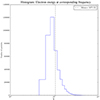 |
Fig. 2. Number of particles per energy in dimensionless units5 corresponding to an observational frequency of νobs = 86 GHz. The mean energy bin, denoted by the dashed vertical line, excludes a large number of particles (that have cooled out of the range of interest) from our emission calculations. |
[5]The energy bin represents the electron Lorentz factor when applying electron rest mass energy units.
Finally, our post-processing analysis results in values for Ne, γmin, and α at irregular macro-particle positions within the jet flow of our hybrid fluid-particle simulation. We then interpolated these values to create a continuous 3D Cartesian grid. This grid is used by RADMC-3D to generate synthetic synchrotron emission maps. Our post-processing enhances our synthetic polarized maps, making them more comparable to observational data. The variable spectral index accounts for cooling effects visible when comparing different observational frequencies (illustrated in Appendix C). In particular, we computed a variable spectral index cube that represents different spectral indices in different regions within the jet.
We considered a specific epoch of the jet simulation that is illustrated in Figure 3, in which the jet’s hot spot or terminal shock has not yet propagated off the grid. The figure shows a 2D slice through the 3D jet simulation and (overlaid) particle population. The particle distribution is color-coded by energy on top of the thermal fluid density, both in dimensionless grid units. The particle distribution, injected into the simulation through the jet nozzle, follows the motion and speed of the underlying fluid, including the backflow motion of the jet. The particles follow the jet stream, for instance, passing through recollimation shocks.
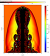 |
Fig. 3. 2D slice of a 3D hybrid fluid-particle simulation. The underlying fluid is color-coded by density in dimensionless grid units. The overplotted particle population is color-coded by averaged particle energy in dimensionless grid units, following the underlying jet stream. The figure shows simulation epoch 38, which represents the last epoch before the jet stream moves off-grid. |
In particular, our post-process calculations are summarized (sequentially) in Fig. 4:
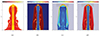 |
Fig. 4. From left to right: Demonstration of our synthetic imaging pipeline. All panels show a 2D slice through our 3D jet simulations. The pipeline starts to extract the particle population from the underlying fluid (see Fig. 3). The particle population in panel (a) is color-coded by dimensionless averaged particle energy. Brighter colors (white and yellow) represent higher energies, i.e., the case for the inner jet spine. The recollimation shock, associated with a centralized region of higher energy, is visible in the jet’s spine. The particles are “cooled” by radiative losses (orange and red) and cool even more rapidly when leaving the jet flow. Panels (b)–(d) illustrate the interpolated particle values that form a grid of particle attributes (highest values in red): Panel (b) shows a 3D grid of the spectral index, α, calculated from the spectrum’s slope, s, of the energetic changes due to radiative losses at a given frequency. Panel (c) highlights the lower energy cutoff, γmin, of the particle’s energy distribution. Panel (d) shows the calculated normalization constant, Ne, of the energy distribution interpolated onto a 3D grid. |
-
Panel (a): The particle distribution is separated from the underlying fluid and the position of the macro-particle is stored. The distinct particles are illustrated without hard edges. This step highlights the energetic changes of the particles when leaving the jet stream. Additionally, the effect of the recollimation shock, which is the increase in the particle’s energy, can be seen in this panel.
-
Panel (b): We interpolated the spectral index, α (power-law slope, s) from the resultant slope of the energy distribution in Fig. 1 at the electron energy, γ, that corresponds to a set observational frequency, νobs. Our radiative transfer scheme relies on the calculated values for the transfer coefficients presented in Jones & Odell (1977), which implies that we set a limit for the spectral index for strongly cooled particles arbitrarily to α = 1.5. With this, we subsequently defined which particles are removed from all interpolations.
-
Panel (c): Similar to step 2, we interpolated the lower energy cutoff, γmin, that is, the lowest energy bin per particle of the simulated power-law distribution in dimensionless units.
-
Panel (d): In a similar manner, we computed the normalization constant, Ne, from γmin and the power-law index, s (see Eq. 7) of the energy distribution in Eq. (5) at a desired frequency, and therefore at a specific energy.
Finally, we output all three components of the magnetic field Bx, y, z (as well as the strength), the lower energy cutoff, γmin, the normalization constant, Ne, and the spectral index, α, on a 3D Cartesian grid into files adjusted for RADMC-3D. In all our RMHD jet simulations, each computational box consists of 320 × 320 × 400 zones, and we set the viewing distance of the source at a redshift of z = 0.002 (the redshift of Centaurus A, Rothschild et al. 2011). The individual scaled cell size is 0.01 parsec (pc). For all the images presented in Sect. 4, we used an observing frequency of νobs = 86 GHz.
3. Synthetic polarized emission calculations
RADMC-3D is a thoroughly tested and well-documented ray-tracing code for solving astrophysical radiative transfer problems (Dullemond et al. 2012). RADMC-3D computes the Stokes parameters I, Q, U, and V (total intensity, LP, and CP, respectively) along individual rays. A modified version of the code accounts for synchrotron absorption, emissivity, Faraday conversion, as well as Faraday rotation (MacDonald & Marscher 2018). The solution of the emitted polarized synchrotron radiation is a function of optical depth, the normalization constant, Ne, the low-energy cutoff, γmin, of the power-law distribution in Eq. (5), the strength of the magnetic field, and its orientation to our line of sight. In contrast to Kramer & MacDonald (2021), we made use of the updated implementation of the full Stokes module in RADMC-3D by MacDonald & Nishikawa (2021). This allows for an additional degree of freedom, namely, a full rotational view of our 3D solution. Finally, we adapted the above described implementation to solve for a variable spectral index. In particular, our solution will apply the radiative transfer calculations to interpolated particle attributes that connect the emitter with the observer. This involves two main steps: (i) a relativistic aberration correction, which is applied cell-by-cell to determine the angle between the local magnetic field vector of each cell and the observer’s orientation relative to the jet axis, and (ii) a rotation correction, which is applied in the same way to convert the LP ellipse from the local comoving frame onto the plane of the sky. Further details on these corrections are published in MacDonald & Nishikawa (2021)5.
Once the Stokes parameters are computed for each line of sight (corresponding to each pixel/ray in our synthetic maps), a Doppler factor is introduced (see Eq. (10)). This factor accounts for the bulk Lorentz factor and orientation of the large-scale jet structure and is used to transform the flux levels into the observer’s frame.
4. Hybrid fluid-particle jet simulation results
4.1. Centaurus A as a laboratory
Centaurus A (Cen A) is one of the earliest known radio galaxies (Clarke et al. 1992), and is located at a distance of approximately 3.8 million parsecs (z = 0.002 Harris et al. 2010; Rothschild et al. 2011). It hosts a SMBH at its core with an estimated mass of about 55 million solar masses (Neumayer 2010). Cen A offers a rich field for multiwavelength observations, though this paper primarily explores its radio characteristics. Cen A features strong jets visible in both the radio and X-ray spectra, spanning from sub-parsecs to hundreds of parsecs in scale (Clarke et al. 1992; Hardcastle et al. 2003; Feain et al. 2011; Müller et al. 2011, 2014; Ehlert et al. 2022). The jet’s observed inclination ranges from i ∈ [12 − 45]° (Müller et al. 2014), with edge-brightening supporting a spine-sheath jet structure (Janssen et al. 2021; Laing et al. 1999). We set our simulated jet’s inclination to i = 35.5°. Cen A is an exemplary case study for AGN research in numerical simulations, particularly for assessing the impact of synchrotron losses in relativistic jet models.
4.2. The effect of synchrotron cooling
The PLUTO code can keep track of an optional jet tracer value for each cell in the simulated Eulerian grid, ranging from zero (in the ambient medium) to one (in the jet). A value close to one indicates that the cell belongs to the jet, while a value close to zero indicates a high presence of ambient medium. By selecting a cutoff value near unity, we can exclude the ambient medium from the input grid that RADMC-3D uses for ray-tracing when creating full Stokes emission maps. This exclusion was necessary for the non-hybrid jet simulations presented in Kramer & MacDonald (2021), where we did not account for the effect of synchrotron cooling (specifically, a cutoff value of 0.75 was used; see the middle panel in Fig. 5)6. Consequently, in these initial calculations, the ambient medium does not cool over time and emits a large amount of synchrotron emission, which obscures our view of the inner jet spine (i.e., with no tracer; see the top panel of Fig. 5). An alternative view of this is illustrated in Fig. A.1. As a result, the jet is entirely obscured by the ambient medium in the absence of synchrotron cooling.
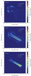 |
Fig. 5. Synthetic total intensity map of the 3D RMHD jet simulation. Top: Map of the 3D RMHD jet simulation generated without the use of a jet tracer, mainly illustrating the emission of the ambient medium. Middle: Map of the jet simulation generated by applying an arbitrarily chosen jet tracer to exclude the ambient medium, highlighting an edge-brightened jet. Bottom: Final 3D hybrid fluid-particle jet simulation, showing an edge-brightened jet emission with the ambient medium excluded by including radiative losses. All maps are ray-traced at 86 GHz and viewed at an observational angle of 35.5°. |
In contrast, when we incorporate synchrotron cooling (via our hybrid fluid-particle simulation), we can clearly observe the jet distinctly from the ambient medium (e.g., bottom panel of Fig. 5). This was achieved without using any jet tracer to arbitrarily exclude the emission of the ambient medium. The emission calculated solely from particle attributes confirms our findings in Kramer & MacDonald (2021), that the toroidal magnetic field configuration consistently results in emission concentrated along the edges of the jet. The simulations in this work produce an edge-brightened appearance in all presented synthetic synchrotron emission maps. Furthermore, the presence of both positive and negative CP, visible in the jet emission, indicates the changing orientation of the jet’s magnetic field relative to our line of sight (see Fig. 6).
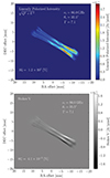 |
Fig. 6. Ray-traced images of our hybrid fluid-particle jet propagating from the bottom right to the top left in linearly polarized intensity (top) and CP (bottom). The pictures illustrate the jet viewed at an observational viewing angle of 35.5° at 86 GHz. The fractional linear (ml) and circular (mc) polarization level is given in the bottom-left corner of each map. |
4.3. Synthetic synchrotron emission maps
In our hybrid fluid-particle simulation, we once again investigated a toroidal magnetic field morphology within the jet. We selected the toroidal magnetic field configuration to replicate the edge-brightening effect observed in the radio galaxy Centaurus A (Janssen et al. 2021; Kramer & MacDonald 2021). In Fig. 5, we compare the results of the non-particle approach, depicted in the top and middle panels (with and without a jet tracer, respectively), to the corresponding images obtained from the hybrid fluid-particle simulations, illustrated in the bottom panel. The figures display the total intensity of the jet’s emission at an inclination of i = 35.5°, observed at 86 GHz (alternative frequencies are presented in Fig. C.1 and discussed in Appendix C). The image clearly demonstrates that the use of a tracer is unnecessary if the simulation accounts for radiative losses. This is stressed as we observe a distinct and well-defined jet structure in the hybrid fluid-particle simulation. We can further compare the resultant brightness (in Jansky per pixel) of the jet between the different approaches, namely, the hybrid fluid-particle approach and the pure fluid jet. The difference between the bow shock’s luminosity and the rest of the relativistic jet makes a noticeable impact on the resultant brightness. When the bow shock is not excluded from the simulation, it outshines the jet structure completely. The bow shock seems to be two orders of magnitude brighter (i.e., ∼2.4 × 10⁻² Jy/pixel) than the jet structure (∼2.8 × 10⁻⁴ Jy/pixel). The brightness and structure of the hybrid-fluid particle simulation and the RMHD jet simulation (using a jet tracer to exclude the lobe) seem to be in agreement. The relativistic jet is carrying an underlying toroidal magnetic field in all panels depicted in Fig. 5. The resultant structure resembles the results published in Kramer & MacDonald (2021). When the jet is visible, an edge brightened jet structure is observed. Both the hybrid fluid-particle jet and the pure fluid jet show the behavior of maximum luminosity in both edges close to the jet launching in the lower right part of the figures. The hybrid fluid-particle jet excludes more of the upstream-structure of the jet due to opacity effects incorporated into our calculations.
In Fig. 6, we present images of the associated synchrotron polarization. The top panel displays the linearly polarized intensity, which is calculated as the square root of the sum of the squares of the Stokes parameters Q and U. It also includes the electric vector position angles (EVPAs) computed as χ = 0.5arctan(U/Q). The EVPA convey the orientation of the magnetic field. As the viewing angle is i = 35.5°, the jet is partially boosted to or de-boosted away from our line of sight. The lower/left edge of the jet carries EVPAs oriented alongside the jet’s direction, highlighting a magnetic field that takes a turn around that edge. The upper, right edge of the jet shows EVPAs perpendicular to the jet’s direction in the innermost part and a small rotation toward the edges. This is indicative of a magnetic field orientation along the jet before taking another turn around the edges. The bottom panel shows the CP, namely, Stokes V. Similar to Kramer & MacDonald (2021), we observe a flip in sign of CP with one sign on each of the highlighted edges. The lower edge carries a strong negative Stokes V, aligning with EVPAs oriented in the jet direction, whereas the upper edge is positive in Stokes V. This again conveys the underlying toroidal magnetic field configuration.
We computed the integrated levels of fractional polarization, which are flux-weighted averages of the Stokes parameters across the entire jet emission region in each set of images (we followed the formalism presented in Kim et al. 2019). These values are listed to the lower left in the linearly polarized and circularly polarized images of Fig. 6. The values are denoted as  for LP and
  for CP. The fractional LP is ml = 1.2 × 101%, while the fractional CP is mc = 4.1 × 10⁻⁵%. In circularly polarized synchrotron emission, we observe both positive and negative CP, which emphasizes the dynamic changes in the orientation of the jet’s magnetic field relative to our line of sight. This finding in our hybrid fluid-particle jet simulation agrees with the RMHD jet simulation presented in Kramer & MacDonald (2021).
5. Discussion
Our spectral analysis of the particles’ energy over time confirms that the particles in the relativistic jet experience synchrotron losses (see Fig. 1). Notably, higher-energy electrons within the macro-particle exhibit a more rapid cooling rate compared to their lower-energy counterparts. Consequently, the initial spectrum’s high-energy tail experiences decay, leading to a subsequent reduction in the parameter γmax (This finding is confirmed in Dubey et al. 2023).
Furthermore, particles that are impacted by the jet’s recollimation shock are gaining energy (see Fig. 4 second image from left). A comprehensive study on the particle shock acceleration is presented in, for example, Mukherjee et al. (2021), Borse et al. (2021), Giri et al. (2022), and Dubey et al. (2023).
We compared our synthetic polarized emission maps with observational data, focusing on the TANAMI (Ojha et al. 2010) observations by Müller et al. (2014) and the Event Horizon Telescope (EHT) observations by Janssen et al. (2021). The interpretation of the brightest jet features as the radio core is favored by Janssen et al. (2021), implying the presence of a stationary shock feature. They consider this a likely explanation for their EHT observations, given the small scales captured in the image presented in Janssen et al. (2021), the high observation frequency, and the closeness of the source. However, they do not eliminate the prospect of insufficient particle acceleration being the main driver for the brightest jet features.
Müller et al. (2014) discovered a prominently bright jet feature, Jstat, situated approximately 3.5 milliarcseconds (mas) downstream from the core, observed to remain stationary relative to the core. This feature’s position could possibly be identified with our simulation’s brightest feature, potentially aligning it with either the radio core observed by Müller et al. (2014) or their Jstat component. If our simulated jet nozzle corresponds to the radio core, the 3.5 mas distance would accurately represent Jstat. Tingay & Murphy (2001) also observed this component, referred to as C3. Jstat could be interpreted as a “cross-shock”7 in the jet flow, similar to phenomena observed in simulations of over-pressured jets (Mimica et al. 2009), where a spectral inversion occurs at recollimation shocks, leading to the acceleration of components in subsequent expansions. Although our simulations do show a recollimation shock in the underlying RMHD simulation, our interpretation diverges. We attribute this phenomenon mainly to the accumulation and amplification of synchrotron emission around the jet edges, driven by the presence of a toroidal magnetic field component. Notably, our numerical model reproduces the observed emission without requiring the introduction of any strong shock acceleration. We stress that a purely toroidal magnetic field configuration would yield symmetric edge-brightened emission spanning the jet, as discussed in Gabuzda (2018). Conversely, a helical magnetic field configuration would lead to more asymmetric emission along the jet edges. This is confirmed in numerical simulations by Kramer & MacDonald (2021), and in the work presented in this paper. We validated the edge-brightened structure of an underlying toroidal magnetic field configuration when calculating the synthetic polarized synchrotron emission from NTP attributes directly. We, moreover, infer that the intrinsic magnetic field morphology is toroidal in nature due to the edge-brightened profile observed by Müller et al. (2014) and Janssen et al. (2021).
Our perspective aligns with the interpretation on the total intensity outlined in Janssen et al. (2021), as we also observe a “core” shift in the peak of Stokes I and linearly polarized intensity as we transition from lower to higher frequencies (from 15 GHz to 230 GHz; see Fig. C.1). We observe that the jet appears optically thick upstream, while downstream, it becomes optically thin. Janssen et al. (2021) identifies the most prominent features within the jet as radio cores, signifying the boundary between regions of upstream synchrotron self-absorption and downstream optically thin regions. They managed to resolve the self-absorbed section between the proposed radio core and the jet apex, a location that coincides with the presence of the SMBH and its accretion disk8. The interpretation of the brightest jet feature as a radio core, given their data, indeed appears to be the most plausible explanation. According to jet theory, a luminous radio core should be observable in very long baseline interferometry images. This phenomenon is a common occurrence in sources resembling Centaurus A, and the core shift usually adheres to the standard ν−1 relation, consistent with most sources (Sokolovsky et al. 2011).
Furthermore, our spectral index cube in Fig. 4b, which interpolates particle attributes across a 3D domain, alongside the jet’s edge-brightening, suggests a transition in opacity from the inner relativistic jet flow to the surrounding backflow material. This phenomenon aligns with the concept of a spine-sheath jet structure (e.g., Laing et al. 1999; Ghisellini 2013; Müller et al. 2014), where a faster-moving spine becomes visible due to its smaller optical depth. Worrall et al. (2008) also noted a steeper spectrum in the jet’s outer layers, reinforcing the idea of a spine-sheath configuration for jets at the 100 pc scale.
Overall, Müller et al. (2014) observed jet emission extending up to approximately 70 mas, or about 1.3 pc, displaying a straight and well-collimated shape without significant bends. This is confirmed by our simulations, revealing a stable, collimated outflow up to several parsec away from the jet launching (nozzle) region.
Our simulations indicate that Cen A presents the potential to reveal a polarized signal up to  (Fig. 6) in fractional linear polarization and
  in fractional CP within its compact jet region, information that is currently unavailable in observations. Acquiring these data is crucial for investigating the behavior of the magnetic field on the inferred scales and assessing the validity of the strong toroidal component generating a bi-modal EVPA pattern and a switch in sign of circularly polarized synchrotron emission. Furthermore, if beam depolarization is responsible for the non-detection of polarization observed by the Atacama Large Millimeter Array (ALMA), conducting observations at 43 GHz wavelength might offer one of the most promising opportunities for polarization detection. This is due to the anticipated detection of the bright jet sheath with a relatively small beam size. 86 GHz observations could serve as calibrator and to validate a possible outcome of nonzero polarization in Centaurus A.
6. Conclusion
We used the PLUTO code (Mignone et al. 2007) to compute 3D RMHD simulations with a Lagrangian particle module (Vaidya et al. 2018). An analysis of the energy distribution of particles over time reveals the impact of synchrotron losses on both the particles within the ambient medium and those within the relativistic jet. To generate ray-traced full Stokes images from these fluid-particle hybrid jet simulations, we performed an interpolation of discrete particle energy and particle number density values across particle positions. Subsequently, these interpolated values were mapped onto continuous Cartesian grids, which were further employed as inputs for the ray-tracing code RADMC-3D. This process allowed us to construct a variable spectral index cube. Importantly, the hybrid fluid-particle jet methodology enables the generation of synthetic emission maps that emphasize the jet’s (polarized) synchrotron emission, obviating the need for the arbitrary “jet tracer” commonly employed in conventional approaches to exclude the ambient medium. This is particularly significant as, in the context of 3D relativistic MHD simulations, the presence of the ambient medium, in the absence of synchrotron losses, can obscure the jet.
The conclusions drawn from our study can be summarized as follows:
-
We calculated the synthetic polarized synchrotron emission directly from NTP attributes and verify the presence of the edge-brightened structure, which corresponds to an underlying toroidal magnetic field configuration (Kramer & MacDonald 2021).
-
Our calculations suggest that the edge-brightened jet structure apparent in EHT observations of Centaurus A (Janssen et al. 2021) can be attributed to the presence of a large-scale helical magnetic field within the jet. A dominant toroidal field component is favored. This is achieved without the need to introduce any substantial shock acceleration (see, e.g., Fig. C.1).
-
From the nearly symmetric brightness profile observed in the data by Janssen et al. (2021), we infer that the intrinsic magnetic field morphology in Centaurus A is most likely toroidal in nature.
-
Our observations reveal a variation in the total intensity peak as we move from lower to higher frequencies, indicating a “core” shift. Meanwhile, we also note that the jet is optically thick upstream but becomes optically thin downstream (see Fig. C.1).
Future refinements will involve: adjusting the Lorentz factor to better match the characteristics of Centaurus A; incorporating shock acceleration to improve the accuracy of the spectral index map across the grid (although the difference is not major, the toroidal magnetic field configuration lacks a recollimation shock); making dimensional adjustments to align our polarized maps with the field of view in the EHT observations; and proposing new observations at 86 GHz of Centaurus A to complement and enhance our study.
It is assumed that scattering in the rest frame of relativistic particles follows the Thompson scattering model and the cosmic background radiation is isotropic.
We computed spectral index “cubes” that are input into RADMC-3D for the post-process ray-tracing.
The Lorentz factor equals the energy bins in the numerical framework.
We would like to emphasize that we numerically excluded shock acceleration and that, hence, the spectrum displays energetic losses only.
Please note that we do not apply a slow-light approach in this work.
It is noteworthy that an additional cut of the grid is applied to the data in order to exclude the jet’s bulk in Kramer & MacDonald (2021).
Cross-shock features are expected to exhibit a spectral inversion linked to recollimation shocks, where components passing through are accelerated in subsequent expansions (Müller et al. 2014).
It is important to acknowledge that with existing telescopes, the radio core and upstream region typically remain unresolved for the majority of AGN.
Acknowledgments
J.A.K.’s research was supported through a PhD grant from the International Max Planck Research School (IMPRS) for Astronomy and Astrophysics at the Universities of Bonn and Cologne, Germany. She is supported for her research by a NASA/ATP project. The LA-UR number is LA-UR-24-22728. The 3D jet simulations presented in this paper have been performed using the PLUTO Code. The calculations were performed on the Raven high performance cluster at the Max Planck Computing and Data Facility. The ray-tracing software RADMC-3D was used to generate the polarized images of the synchrotron emission. The authors thank B. Vaidya and D. Mukherjee for important and thoughtful discussions on the results presented in this work. The authors are grateful to E. Ros for comments and M. Janssen for insights on Centaurus A. G.F.P. acknowledges support by the European Research Council advanced grant “M2FINDERS – Mapping Magnetic Fields with INterferometry Down to Event hoRizon Scales” (Grant No. 101018682). L.R. is funded by the Deutsche Forschungsgemeinschaft (DFG, German Research Foundation)–project number 443220636.
References
- Bai, X.-N., Caprioli, D., Sironi, L., & Spitkovsky, A. 2015, ApJ, 809, 55 [NASA ADS] [CrossRef] [Google Scholar]
- Bellan, P. M. 2018, Phys. Plasmas, 25, 055601 [NASA ADS] [CrossRef] [Google Scholar]
- Blandford, R. D., & Rees, M. J. 1974, MNRAS, 169, 395 [NASA ADS] [CrossRef] [Google Scholar]
- Borse, N., Acharya, S., Vaidya, B., et al. 2021, A&A, 649, A150 [NASA ADS] [CrossRef] [EDP Sciences] [Google Scholar]
- Brunetti, G., Mack, K. H., Prieto, M. A., & Varano, S. 2003, MNRAS, 345, L40 [CrossRef] [Google Scholar]
- Carilli, C. L., Kurk, J. D., van der Werf, P. P., Perley, R. A., & Miley, G. K. 1999, AJ, 118, 2581 [NASA ADS] [CrossRef] [Google Scholar]
- Clarke, D. A., Burns, J. O., & Norman, M. L. 1992, ApJ, 395, 444 [NASA ADS] [CrossRef] [Google Scholar]
- Condon, J. J., & Ransom, S. M. 2016, Essential Radio Astronomy (Princeton: Princeton University Press) [Google Scholar]
- Crew, G. B., Goddi, C., Matthews, L. D., et al. 2023, PASP, 135, 025002 [NASA ADS] [CrossRef] [Google Scholar]
- Daldorff, L. K. S., Tóth, G., Gombosi, T. I., et al. 2014, J. Comput. Phys., 268, 236 [NASA ADS] [CrossRef] [Google Scholar]
- de la Cita, V. M., Bosch-Ramon, V., Paredes-Fortuny, X., Khangulyan, D., & Perucho, M. 2016, A&A, 591, A15 [NASA ADS] [CrossRef] [EDP Sciences] [Google Scholar]
- Dubey, R. P., Fendt, C., & Vaidya, B. 2023, ApJ, 952, 1 [NASA ADS] [CrossRef] [Google Scholar]
- Dullemond, C. P., Juhasz, A., Pohl, A., et al. 2012, Astrophysics Source Code Library [record ascl:1202.015] [Google Scholar]
- Ehlert, S. R., Ferrazzoli, R., Marinucci, A., et al. 2022, ApJ, 935, 116 [NASA ADS] [CrossRef] [Google Scholar]
- EHT MWL Science Working Group (Algaba, J. C., et al.) 2021, ApJ, 911, L11 [NASA ADS] [CrossRef] [Google Scholar]
- Feain, I. J., Cornwell, T. J., Ekers, R. D., et al. 2011, ApJ, 740, 17 [NASA ADS] [CrossRef] [Google Scholar]
- Fromm, C. M., Perucho, M., Mimica, P., & Ros, E. 2016, A&A, 588, A101 [NASA ADS] [CrossRef] [EDP Sciences] [Google Scholar]
- Gabuzda, D. 2018, Galaxies, 6, 9 [NASA ADS] [CrossRef] [Google Scholar]
- Gabuzda, D. C., Vitrishchak, V. M., Mahmud, M., & O’Sullivan, S. 2008, ASP Conf. Ser., 386, 444 [NASA ADS] [Google Scholar]
- Ghisellini, G. 2013, EPJ Web Conf., 61, 05001 [NASA ADS] [CrossRef] [EDP Sciences] [Google Scholar]
- Giri, G., Dubey, R. P., Rubinur, K., Vaidya, B., & Kharb, P. 2022, MNRAS, 514, 5625 [NASA ADS] [CrossRef] [Google Scholar]
- Hada, K., Doi, A., Kino, M., et al. 2011, Nature, 477, 185 [NASA ADS] [CrossRef] [Google Scholar]
- Hardcastle, M. J., Worrall, D. M., Kraft, R. P., et al. 2003, ApJ, 593, 169 [NASA ADS] [CrossRef] [Google Scholar]
- Harris, G. L. H., Rejkuba, M., & Harris, W. E. 2010, PASA, 27, 457 [NASA ADS] [CrossRef] [Google Scholar]
- Heavens, A. F., & Meisenheimer, K. 1987, MNRAS, 225, 335 [NASA ADS] [Google Scholar]
- Hirotani, K., Takahashi, M., Nitta, S.-Y., & Tomimatsu, A. 1992, ApJ, 386, 455 [NASA ADS] [CrossRef] [Google Scholar]
- Homan, D., Hovatta, T., Kovalev, Y., et al. 2018, Galaxies, 6, 17 [NASA ADS] [CrossRef] [Google Scholar]
- Janssen, M., Falcke, H., Kadler, M., et al. 2021, Nat. Astron., 5, 1017 [NASA ADS] [CrossRef] [Google Scholar]
- Jones, T. W., & Odell, S. L. 1977, A&A, 61, 291 [NASA ADS] [Google Scholar]
- Kang, H., Jones, T. W., & Ryu, D. 1992, ApJ, 385, 193 [NASA ADS] [CrossRef] [Google Scholar]
- Kim, J.-Y., Krichbaum, T. P., Marscher, A. P., et al. 2019, A&A, 622, A196 [NASA ADS] [CrossRef] [EDP Sciences] [Google Scholar]
- Kim, D.-W., Janssen, M., Krichbaum, T. P., et al. 2023, A&A, 680, L3 [NASA ADS] [CrossRef] [EDP Sciences] [Google Scholar]
- Kramer, J. A., & MacDonald, N. R. 2021, A&A, 656, A143 [NASA ADS] [CrossRef] [EDP Sciences] [Google Scholar]
- Laing, R. A., Parma, P., Ruiter, H. R. D., & Fanti, R. 1999, MNRAS, 306, 513 [NASA ADS] [CrossRef] [Google Scholar]
- Lister, M. L., & Homan, D. C. 2005, AJ, 130, 1389 [NASA ADS] [CrossRef] [Google Scholar]
- Lobanov, A. P. 1998, A&AS, 132, 261 [NASA ADS] [CrossRef] [EDP Sciences] [Google Scholar]
- MacDonald, N. R., & Marscher, A. P. 2018, ApJ, 862, 58 [CrossRef] [Google Scholar]
- MacDonald, N. R., & Nishikawa, K. I. 2021, A&A, 653, A10 [Google Scholar]
- Mandal, A., Mukherjee, D., & Mignone, A. 2023, ApJS, 268, 40 [NASA ADS] [CrossRef] [Google Scholar]
- Mattia, G., Del Zanna, L., Bugli, M., et al. 2023, A&A, 679, A49 [NASA ADS] [CrossRef] [EDP Sciences] [Google Scholar]
- Meisenheimer, K., & Roeser, H. J. 1986, Nature, 319, 459 [NASA ADS] [CrossRef] [Google Scholar]
- Melon Fuksman, J. D., & Mignone, A. 2019, ApJS, 242, 20 [NASA ADS] [CrossRef] [Google Scholar]
- Mignone, A., Bodo, G., Massaglia, S., et al. 2007, ApJS, 170, 228 [Google Scholar]
- Mignone, A., Bodo, G., Vaidya, B., & Mattia, G. 2018, ApJ, 859, 13 [CrossRef] [Google Scholar]
- Mignone, A., Flock, M., & Vaidya, B. 2019, ApJS, 244, 38 [Google Scholar]
- Mignone, A., Haudemand, H., & Puzzoni, E. 2023, Comput. Phys. Commun., 285, 108625 [NASA ADS] [CrossRef] [Google Scholar]
- Mimica, P., Aloy, M.-A., Agudo, I., et al. 2009, ApJ, 696, 1142 [NASA ADS] [CrossRef] [Google Scholar]
- Mimica, P., Giannios, D., Metzger, B., & Aloy, M. A. 2012, EPJ Web Conf., 39, 04003 [NASA ADS] [CrossRef] [EDP Sciences] [Google Scholar]
- Mizuno, Y., Gómez, J. L., Nishikawa, K.-I., et al. 2015, ApJ, 809, 38 [Google Scholar]
- Mukherjee, D., Bodo, G., Rossi, P., Mignone, A., & Vaidya, B. 2021, MNRAS, 505, 2267 [NASA ADS] [CrossRef] [Google Scholar]
- Müller, C., Kadler, M., Ojha, R., et al. 2011, A&A, 530, L11 [NASA ADS] [CrossRef] [EDP Sciences] [Google Scholar]
- Müller, C., Kadler, M., Ojha, R., et al. 2014, A&A, 569, A115 [NASA ADS] [CrossRef] [EDP Sciences] [Google Scholar]
- Neumayer, N. 2010, PASA, 27, 449 [NASA ADS] [CrossRef] [Google Scholar]
- Nurisso, M., Celotti, A., Mignone, A., & Bodo, G. 2023, MNRAS, 522, 5517 [NASA ADS] [CrossRef] [Google Scholar]
- Ojha, R., Kadler, M., Böck, M., et al. 2010, A&A, 519, A45 [NASA ADS] [CrossRef] [EDP Sciences] [Google Scholar]
- Paraschos, G. F., Kim, J. Y., Krichbaum, T. P., & Zensus, J. A. 2021, A&A, 650, L18 [NASA ADS] [CrossRef] [EDP Sciences] [Google Scholar]
- Paraschos, G. F., Mpisketzis, V., Kim, J. Y., et al. 2023, A&A, 669, A32 [NASA ADS] [CrossRef] [EDP Sciences] [Google Scholar]
- Paraschos, G. F., Debbrecht, L. C., Kramer, J. A., et al. 2024, A&A, 686, L5 [NASA ADS] [CrossRef] [EDP Sciences] [Google Scholar]
- Park, J., & Algaba, J. C. 2022, Galaxies, 10, 102 [NASA ADS] [CrossRef] [Google Scholar]
- Perucho, M., López-Miralles, J., Gizani, N. A. B., Martí, J. M., & Boccardi, B. 2023, MNRAS, 523, 3583 [NASA ADS] [CrossRef] [Google Scholar]
- Pontin, D. I., & Priest, E. R. 2022, Liv. Rev. Sol. Phys., 19, 1 [NASA ADS] [CrossRef] [Google Scholar]
- Porth, O., Fendt, C., Meliani, Z., & Vaidya, B. 2011, ApJ, 737, 42 [Google Scholar]
- Pushkarev, A. B., Gabuzda, D. C., Vetukhnovskaya, Y. N., & Yakimov, V. E. 2005, MNRAS, 356, 859 [Google Scholar]
- Pushkarev, A. B., Hovatta, T., Kovalev, Y. Y., et al. 2012, A&A, 545, A113 [NASA ADS] [CrossRef] [EDP Sciences] [Google Scholar]
- Pushkarev, A., Kovalev, Y., Lister, M., et al. 2017, Galaxies, 5, 93 [NASA ADS] [CrossRef] [Google Scholar]
- Rees, A. I. 1966, J. Geol., 74, 856 [NASA ADS] [CrossRef] [Google Scholar]
- Rothschild, R. E., Markowitz, A., Rivers, E., et al. 2011, ApJ, 733, 23 [NASA ADS] [CrossRef] [Google Scholar]
- Rybicki, G. B., & Lightman, A. P. 1979, Radiative Processes in Astrophysics, 1st edn. (New York: Wiley) [Google Scholar]
- Sokolovsky, K. V., Kovalev, Y. Y., Pushkarev, A. B., & Lobanov, A. P. 2011, A&A, 532, A38 [CrossRef] [EDP Sciences] [Google Scholar]
- Sow Mondal, S., Sarkar, A., Vaidya, B., & Mignone, A. 2023, AAS/Solar Physics Division Meeting, 55, 106.30 [NASA ADS] [Google Scholar]
- Tingay, S. J., & Murphy, D. W. 2001, ApJ, 546, 210 [NASA ADS] [CrossRef] [Google Scholar]
- Todorov, R. V., Kravchenko, E. V., Pashchenko, I. N., & Pushkarev, A. B. 2023, Astron. Rep., 67, 1275 [NASA ADS] [CrossRef] [Google Scholar]
- Tsunetoe, Y., Mineshige, S., Ohsuga, K., Kawashima, T., & Akiyama, K. 2021, PASJ, 73, 912 [NASA ADS] [CrossRef] [Google Scholar]
- Urry, C. M., & Padovani, P. 1995, PASP, 107, 803 [NASA ADS] [CrossRef] [Google Scholar]
- Vaidya, B., Mignone, A., Bodo, G., & Massaglia, S. 2016, J. Phys. Conf. Ser., 719, 012023 [NASA ADS] [CrossRef] [Google Scholar]
- Vaidya, B., Mignone, A., Bodo, G., Rossi, P., & Massaglia, S. 2018, ApJ, 865, 144 [Google Scholar]
- van Marle, A. J., Casse, F., & Marcowith, A. 2018, MNRAS, 473, 3394 [NASA ADS] [CrossRef] [Google Scholar]
- Wardle, J. F. C., Homan, D. C., Ojha, R., & Roberts, D. H. 1998, Nature, 395, 457 [NASA ADS] [CrossRef] [Google Scholar]
- Webb, G. M. 1989, ApJ, 340, 1112 [Google Scholar]
- Worrall, D. M., Birkinshaw, M., Kraft, R. P., et al. 2008, ApJ, 673, L135 [NASA ADS] [CrossRef] [Google Scholar]
Appendix A: Structure
An underlying structure comes to light when employing a logarithmic scale in our analysis: the edge-brightened jet structure is distinct and can be indeed observed through the dense cocoon, as illustrated in Fig. A.1. This figure shows a comprehensive view of a total intensity map derived from a preceding 3D RMHD jet simulation (Kramer & MacDonald 2021). It is noteworthy that this outcome is achieved without the use of any specialized jet tracer or intricate particle physics mechanisms. One prominent feature highlighted in the figure is the bow shock, which, under these circumstances, completely overshadows the jet structure. However, by considering radiative losses, a physical effect takes place. The bow shock, which comprises particles flowing in reverse, undergoes a cooling process, leading to a reduction in its intensity and overall prominence. This insight stresses the complex interplay between various physical factors that ultimately shape the observable characteristics of the jet and its surrounding environment. Figure A.1 proves that we are indeed using the very same numerical setup, and that we can obtain the result of an unobscured edge-brightened jet when we choose the hybrid fluid-particle approach.
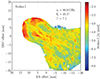 |
Fig. A.1. Resolved 86 GHz total intensity maps of the 3D RMHD jet simulation presented in Kramer & MacDonald (2021) in logarithmic color-coding. The jet emission is viewed at an observational viewing angle of 35.5°. The logarithmic plot reveals an edge-brightening jet hidden behind the bow shock. |
Appendix B: Particle shock acceleration
Although our paper focuses on the importance of radiative losses through the inclusion of particle physics, the impact of particle shock acceleration is also significant. This form of acceleration is crucial in the presence of phenomena like a recollimation shock, a plasmoid moving through the jet, magnetic reconnection events, or instabilities (Borse et al. 2021; Mukherjee et al. 2021). It is noteworthy that our initialization of the spectral index value, namely α = 2, mimics a flat spectrum and does not enhance particle acceleration (flattening of the spectrum) too strongly. We chose this value based on radio observations (see, e.g., Paraschos et al. 2021). Furthermore, our simulations, which utilize a purely toroidal magnetic field, do not exhibit any features that would significantly influence particle acceleration, as discussed in Kramer & MacDonald (2021). The synthetic polarized emission strengthens toward the jet edges, suggesting that particles cluster around the toroidal magnetic field lines. Figure B.1 displays structures similar to those in Fig. 5, notably an edge-brightened jet structure. Including particle acceleration mechanisms such as diffusive shock acceleration would further highlight the jet emission, especially emphasizing the strong bow shock moving through the ambient medium (Giri et al. 2022). We also confirm higher values of total intensity due to the presence of the strong bow shock, visible in Fig. 5 as well. For a more detailed discussion on shock acceleration, we refer the reader to studies like those by, for example, Dubey et al. (2023), Mattia et al. (2023), and Giri et al. (2022).
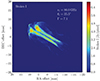 |
Fig. B.1. Resolved 86 GHz total intensity maps of the 3D hybrid fluid-particle jet simulation with the inclusion of particle shock acceleration. The jet emission is viewed at an observational viewing angle of 35.5°. The inclusion of acceleration mechanisms reveals the highlighted bow shock in addition to the edge-brightened jet. |
Appendix C: Frequency
Our observations of the polarized total intensity maps of synthetic synchrotron emission shown in Fig. C.1 reveal several key characteristics of the jet’s emission. Specifically, the emission pattern displays edge-brightening, an effect that can be attributed to the presence of a toroidal magnetic field configuration (Laing et al. 1999). Notably, this distinctive feature highlights the physical insights into jet collimation that can be gained from RMHD simulations (Gabuzda 2018; Pushkarev et al. 2005).
Our analysis also reveals an opacity effect within the compact region. This effect is commonly referred to as "core shift" and is a phenomenon manifested as the apparent shift of the unresolved compact region toward the central engine, with increasing observing frequency (Lobanov 1998; Hirotani et al. 1992; Hada et al. 2011; Pushkarev et al. 2005, 2017; Paraschos et al. 2021; Park & Algaba 2022; Paraschos et al. 2023). Such higher frequency observations can peer deeper into synchrotron self-absorbed sources, as they then appear less opaque. Below we distinguish between two cases (case I and II) for the nature of the “radio core”.
In case I we defined the unresolved region as the radio core at the peak brightness point of the emission. We detect a discernible shift of the radio core position toward the central engine when moving to higher frequencies (from 1 GHz to 15 GHz and 86 GHz to 230 GHz).
Alternatively, in case II, the radio core is considered to be the boundary between regions of upstream synchrotron self-absorption and downstream optically thin segments; then a compelling argument emerges. In this context, identifying the radio core with the location of the recollimation shock becomes a plausible proposition, as can be seen in the most left panel in Fig. 4. If that scenario is correct, studying radio cores with very long baseline interferometry can reveal new insights into jet launching.
Finally, a noteworthy trend comes to light in our simulations: the jet’s observed brightness progressively diminishes, as we ascend toward higher frequencies. This suggests that our analysis of the jet is in the optically thin regime, beyond the turnover frequency. As the observing capabilities of state-of-the-art arrays like the EHT expand into ever higher frequencies (see, e.g., Crew et al. 2023), insights into the jet physics in the optically thin regime will be crucial. Simulations like the ones presented here are primed to advance our understanding of the nature of jets.
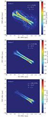 |
Fig. C.1. Resolved total intensity maps of the final 3D hybrid fluid-particle jet simulation revealing an edge-brightened jet emission in 1 GHz (top), 15 GHz (middle), and 230 GHz (bottom). All three maps are viewed at an observational viewing angle of 35.5°. The figure highlights the influence opacity effects have on resultant synthetic synchrotron emission. |
All Figures
|
Fig. 1. Normalized spectral distribution in dimensionless grid units of a representative macro-particle. The corresponding Lagrangian particle is located in the jet’s spine just before entering the back-flow. The initial energy bins are chosen to be within 10 ≤ γ ≤ 107. The particle is injected onto the grid through the jet orifice at epoch 20 (each color represents a different simulation epoch). The radiative losses experienced by this NTP are visible as the particle’s energy distribution evolves (in time) from right to left. |
| In the text | |
|
Fig. 2. Number of particles per energy in dimensionless units5 corresponding to an observational frequency of νobs = 86 GHz. The mean energy bin, denoted by the dashed vertical line, excludes a large number of particles (that have cooled out of the range of interest) from our emission calculations. |
| In the text | |
|
Fig. 3. 2D slice of a 3D hybrid fluid-particle simulation. The underlying fluid is color-coded by density in dimensionless grid units. The overplotted particle population is color-coded by averaged particle energy in dimensionless grid units, following the underlying jet stream. The figure shows simulation epoch 38, which represents the last epoch before the jet stream moves off-grid. |
| In the text | |
|
Fig. 4. From left to right: Demonstration of our synthetic imaging pipeline. All panels show a 2D slice through our 3D jet simulations. The pipeline starts to extract the particle population from the underlying fluid (see Fig. 3). The particle population in panel (a) is color-coded by dimensionless averaged particle energy. Brighter colors (white and yellow) represent higher energies, i.e., the case for the inner jet spine. The recollimation shock, associated with a centralized region of higher energy, is visible in the jet’s spine. The particles are “cooled” by radiative losses (orange and red) and cool even more rapidly when leaving the jet flow. Panels (b)–(d) illustrate the interpolated particle values that form a grid of particle attributes (highest values in red): Panel (b) shows a 3D grid of the spectral index, α, calculated from the spectrum’s slope, s, of the energetic changes due to radiative losses at a given frequency. Panel (c) highlights the lower energy cutoff, γmin, of the particle’s energy distribution. Panel (d) shows the calculated normalization constant, Ne, of the energy distribution interpolated onto a 3D grid. |
| In the text | |
|
Fig. 5. Synthetic total intensity map of the 3D RMHD jet simulation. Top: Map of the 3D RMHD jet simulation generated without the use of a jet tracer, mainly illustrating the emission of the ambient medium. Middle: Map of the jet simulation generated by applying an arbitrarily chosen jet tracer to exclude the ambient medium, highlighting an edge-brightened jet. Bottom: Final 3D hybrid fluid-particle jet simulation, showing an edge-brightened jet emission with the ambient medium excluded by including radiative losses. All maps are ray-traced at 86 GHz and viewed at an observational angle of 35.5°. |
| In the text | |
|
Fig. 6. Ray-traced images of our hybrid fluid-particle jet propagating from the bottom right to the top left in linearly polarized intensity (top) and CP (bottom). The pictures illustrate the jet viewed at an observational viewing angle of 35.5° at 86 GHz. The fractional linear (ml) and circular (mc) polarization level is given in the bottom-left corner of each map. |
| In the text | |
|
Fig. A.1. Resolved 86 GHz total intensity maps of the 3D RMHD jet simulation presented in Kramer & MacDonald (2021) in logarithmic color-coding. The jet emission is viewed at an observational viewing angle of 35.5°. The logarithmic plot reveals an edge-brightening jet hidden behind the bow shock. |
| In the text | |
|
Fig. B.1. Resolved 86 GHz total intensity maps of the 3D hybrid fluid-particle jet simulation with the inclusion of particle shock acceleration. The jet emission is viewed at an observational viewing angle of 35.5°. The inclusion of acceleration mechanisms reveals the highlighted bow shock in addition to the edge-brightened jet. |
| In the text | |
|
Fig. C.1. Resolved total intensity maps of the final 3D hybrid fluid-particle jet simulation revealing an edge-brightened jet emission in 1 GHz (top), 15 GHz (middle), and 230 GHz (bottom). All three maps are viewed at an observational viewing angle of 35.5°. The figure highlights the influence opacity effects have on resultant synthetic synchrotron emission. |
| In the text | |
Current usage metrics show cumulative count of Article Views (full-text article views including HTML views, PDF and ePub downloads, according to the available data) and Abstracts Views on Vision4Press platform.
Data correspond to usage on the plateform after 2015. The current usage metrics is available 48-96 hours after online publication and is updated daily on week days.
Initial download of the metrics may take a while.