| Issue |
A&A
Volume 622, February 2019
|
|
|---|---|---|
| Article Number | A30 | |
| Number of page(s) | 18 | |
| Section | Extragalactic astronomy | |
| DOI | https://doi.org/10.1051/0004-6361/201834260 | |
| Published online | 24 January 2019 | |
Hyper Suprime-Cam view of the CMASS galaxy sample
Halo mass as a function of stellar mass, size, and Sérsic index
1
Leiden Observatory, Leiden University, Niels Bohrweg 2, 2333 CA Leiden, The Netherlands
e-mail: This email address is being protected from spambots. You need JavaScript enabled to view it.
2
Kavli IPMU (WPI), UTIAS, The University of Tokyo, Kashiwa, Chiba 277-8583, Japan
3
Department of Astrophysical Sciences, Princeton University, 4 Ivy Lane, Princeton, NJ 08544, USA
Received:
17
September
2018
Accepted:
9
November
2018
Abstract
Aims. We wish to determine the distribution of dark matter halo masses as a function of the stellar mass and the stellar mass profile for massive galaxies in the Baryon Oscillation Spectroscopic Survey (BOSS) constant-mass (CMASS) sample.
Methods. We used grizy photometry from the Hyper Suprime-Cam (HSC) to obtain Sérsic fits and stellar masses of CMASS galaxies for which HSC weak-lensing data are available. This sample was visually selected to have spheroidal morphology. We applied a cut in stellar mass, log M*/M⊙ > 11.0, and selected ∼10 000 objects thus. Using a Bayesian hierarchical inference method, we first investigated the distribution of Sérsic index and size as a function of stellar mass. Then, making use of shear measurements from HSC, we measured the distribution of halo mass as a function of stellar mass, size, and Sérsic index.
Results. Our data reveal a steep stellar mass-size relation Re ∝ M*βR, with βR larger than unity, and a positive correlation between Sérsic index and stellar mass: n ∝ M*0.46. The halo mass scales approximately with the 1.7 power of the stellar mass. We do not find evidence for an additional dependence of halo mass on size or Sérsic index at fixed stellar mass.
Conclusions. Our results disfavour galaxy evolution models that predict significant differences in the size growth efficiency of galaxies living in low- and high-mass halos.
Key words: galaxies: elliptical and lenticular / cD / gravitational lensing: weak / galaxies: fundamental parameters
Marie Skłodowska-Curie Fellow.
© ESO 2019
1. Introduction
The size evolution of massive quiescent galaxies is one of the open questions in cosmology. On the one hand, observations show that at fixed stellar mass, the average size of quiescent galaxies has increased by a factor of a few between z ≈ 2 and the present (e.g. Daddi et al. 2005; Trujillo et al. 2006; van Dokkum et al. 2008). On the other hand, theoretical models have struggled to reproduce this trend (see e.g. Hopkins et al. 2010a). Qualitatively, the size evolution of massive quiescent galaxies is understood to be the result of mergers. Minor mergers, in particular, are known to be an efficient mechanism to increase the size of a galaxy (Naab et al. 2009). However, it is not clear whether the observed merger rates are sufficient to explain the size evolution signal, especially in the redshift range 1 < z < 2 (Newman et al. 2012). Moreover, it is very difficult to preserve the tightness of the stellar mass-size relation observed at z ∼ 0 with evolutionary models that are based exclusively on dissipationless (dry) mergers (Nipoti et al. 2012).
Clues on the physical mechanisms that are relevant for the size evolution of massive galaxies can be obtained by studying the dependence of size on environment (see Shankar et al. 2014a). Although the correlation between environment and galaxy size at fixed stellar mass has been investigated by a relatively large number of studies, no clear consensus has been reached, with some works showing evidence for a positive correlation Cooper et al. (2012), Papovich et al. (2012), Lani et al. (2013), Yoon et al. (2017), Huang et al. (2018a), and others finding results consistent with no dependence Huertas-Company et al. (2013a), Newman et al. (2014), Allen et al. (2015), Damjanov et al. (2015), and Saracco et al. (2017). The signal, if present, is in any case small: reported differences between the average size of galaxies found in clusters and in less massive associations are of the order of 20%.
A possible way forward is looking at correlations between the observed properties of galaxies and those of their host dark matter halos. The evolution of the mass of a dark matter halo directly traces its accretion and merger history. This, in turn, should relate directly to the size evolution of its central galaxy, since mergers are thought to be the main driver of the growth in size, at least at the massive end of the galaxy distribution.
Halo masses can be measured using weak gravitational lensing. However, the low strength of the weak-lensing signal around typical massive galaxies requires the statistical combination of measurements over hundreds or thousands of lenses, making it challenging to obtain an accurate description of the distribution of halo mass as a function of galaxy properties other than stellar mass.
Recently, Charlton et al. (2017) reported the detection of a positive correlation between halo mass and size at fixed stellar mass, using stacked weak-lensing measurements from the Canada-France-Hawaii Telescope Lensing Survey (CFHTLenS; Heymans et al. 2012). Here we use a Bayesian hierarchical inference method to fit for the distribution of halo mass as a function of stellar mass, size, and Sérsic index, using photometric and weak-lensing data from the Hyper Suprime-Cam (HSC) survey (Aihara et al. 2018a).
We draw the lens galaxies used in our study from the constant-mass (CMASS) sample of the Baryon Oscillation Spectroscopic Survey (BOSS, Schlegel et al. 2009; Dawson et al. 2013). The CMASS sample has been used for a variety of studies in galaxy evolution and cosmology (e.g. Anderson et al. 2014; Beutler et al. 2014; More et al. 2015; Montero-Dorta et al. 2016; Leauthaud et al. 2017; Tinker et al. 2017; Favole et al. 2018; Guo et al. 2018). Thanks to the image quality (0.6″ typical i−band seeing) and depth of HSC data, our work will allow us to obtain a more accurate description of the light distribution in CMASS galaxies compared to previous studies. A by-product of our analysis is then a measurement of the stellar mass-size relation of CMASS galaxies, which we generalise to a stellar mass-size-Sérsic index relation based on unprecedented deep and sharp data.
The structure of this work is the following. In Sect. 2 we describe the data used for our study. In Sect. 3 we carry out an investigation on the distribution of Sérsic index and half-light radius as a function of stellar mass. In Sect. 4 we perform a weak-lensing analysis to infer the distribution of dark matter halo mass as a function of various galaxy properties. We discuss our results in Sect. 5 and conclude in Sect. 6. We assume a flat Λ cold dark matter cosmology with ΩM = 0.3 and H0 = 70 km s−1 Mpc−1.
2. Data
2.1. CMASS sample
The set of galaxies that is subject of our study is drawn from the CMASS sample of BOSS, which is part of the Sloan Digital Sky Survey III (SDSS-III, Eisenstein et al. 2011). The CMASS sample has been constructed with the primary goal of selecting luminous red galaxies in the redshift range 0.43 < z < 0.7 for the measurement of the baryon acoustic oscillation signal. CMASS galaxies are selected by applying a series of cuts on colours and magnitudes, as measured from SDSS photometry. We refer to Reid et al. (2016) for details on the selection criteria of the CMASS sample. For each galaxy in the CMASS sample, we have a spectroscopic redshift measured with the BOSS spectrograph.
2.2. HSC photometry
We selected CMASS galaxies that lie in the region covered by the first-year shear catalogue of the HSC survey (Mandelbaum et al. 2018). This corresponds to 136.9 deg2 imaged in grizy bands at the full survey depth (i ∼ 26.4 mag 5σ limit for a point source, Aihara et al. 2018b), resulting in a sample size of approximately 18 000 CMASS galaxies. For each galaxy in the sample, we obtained small cutouts of coadded images in each band from the S17a internal data release. Data reduction, including the generation of coadded images, model point spread function (PSF) kernels, and sky subtraction were performed using HSCPIPE (Bosch et al. 2018), a version of the Large Synoptic Survey Telescope software stack (Ivezic et al. 2008; Axelrod et al. 2010; Jurić et al. 2017). We refer to Bosch et al. (2018) for details on the data reduction process. In Fig. 1 we show colour-composite images of a set of 20 galaxies drawn randomly from the final sample used for our study (the criteria used to define the final sample are listed in the rest of this section).
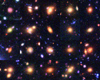 |
Fig. 1. Colour-composite images in HSC-irg bands of a set of 20 galaxies drawn randomly from the sample used for our study. We used the algorithm of Marshall et al. (2016) to create the images. |
2.3. Sérsic profile fits
We fitted an elliptical Sérsic surface brightness profile (Sersic 1968) to the photometric data in each band:
 (1)
(1)
where x and y are Cartesian coordinates aligned with the major and minor axis of the elliptical isophotes and origin in the centre, R is the circularised radius,
 (2)
(2)
n is the Sérsic index, and b(n) is a numerical constant that ensures that the light enclosed within the isophote with R = Re is half of the total light (see Ciotti & Bertin 1999).
For each galaxy, we fixed the parameters of the Sérsic profile to be the same in all five bands, with the exception of the amplitude I0. In other words, we assumed galaxies to have spatially uniform colours. We ran a Markov chain Monte Carlo (MCMC) method to sample the parameter space defined by the galaxy centroid, half-light radius, axis ratio, position angle, Sérsic index, and g − i, r − i, i − z, y − i colours. For each set of values of these structural parameters, we found the i−band amplitude that minimises the following χ2:
 (3)
(3)
where  is the PSF-convolved Sérsic model in band λ evaluated at pixel j, Iλ, j is the observed surface brightness at the corresponding pixel, and σλ, j is the observational uncertainty. Since the model surface brightness is linear in the i−band amplitude, the above χ2 can be minimised analytically.
A circular region of 50 pixel (8.4″) radius centred on each galaxy was used for the fit. This corresponds to a physical radius of 54 kpc at z = 0.55, the median redshift of our sample. The choice of this aperture is a compromise between the need for capturing as much light as possible from each galaxy and at the same time avoiding to select too large a region, in order to avoid being affected by systematics in the sky subtraction. We verified that our results did not change when we used a fitting region larger or smaller by a factor of two.
The model parameters were initialised to the values of the CMODEL_DEV fit produced by HSCPIPE, with n = 4. We ran SEXTRACTOR (Bertin & Arnouts 1996), with a 2σ detection threshold, on the i− and g− band image to mask objects that were not associated with the main galaxy. We ran a preliminary MCMC on the centroid and colour parameters while keeping the Sérsic index, position angle, axis ratio, and half-light radius fixed, ran SEXTRACTOR once again on the model-subtracted image, then ran another MCMC over the full set of parameters. We used the package EMCEE (Foreman-Mackey et al. 2013) to perform the MCMC. Typical statistical uncertainties are 2% on Re and n, 1% on the axis ratio q, ∼1 deg on the position angle and 0.01 mag on the magnitudes.
We wish to carry out our measurements on passive galaxies alone since star-forming galaxies have been shown to lie on a different stellar-to-halo mass relation (Mandelbaum et al. 2016) and could therefore bias our inference. We then visually inspected each CMASS galaxy and removed from the sample any object that showed clear signs of star formation activity or disc-like morphology. We also discarded systems on which it was difficult to carry out photometric measurements in an automated way, such as blended objects, images with significant contamination from a nearby bright star, or strong gravitational lenses. After this visual inspection step, we were left with ∼13 000 elliptical galaxies with clean photometry.
2.4. Stellar masses
We estimated stellar masses by fitting synthetic stellar population models to the observed grizy magnitudes, following the procedure described by Auger et al. (2009), with minor modifications. We took simple stellar population (SSPs, or instantaneous-burst) models, produced by Bruzual & Charlot (2003) using semi-empirical stellar spectra from the BaSeL 3.1 library (Westera et al. 2002) and the Padova 1994 evolutionary tracks, assuming a Chabrier initial mass function (IMF, Chabrier 2003). We then used the BC03 code (Bruzual & Charlot 2003) to create composite stellar population (CSP) model spectra, assuming an exponentially decaying star formation history, over a four-dimensional grid of age (i.e. time since the initial burst), star formation rate decay time τ, metallicity Z, and dust attenuation τV. We used these synthetic spectra to evaluate the model broadband flux in each HSC filter at each point of the grid, adding redshift as a fifth dimension. Finally, we fitted for stellar mass, age, τ, metallicity, and dust attenuation by running an MCMC: for each set of values of the model parameters, we obtained the predicted grizy magnitudes by interpolating over the grid, and compared them to the observed values.
Thanks to the depth of HSC data, the typical observational uncertainties on the fluxes are ∼0.01 mag. This is a much lower value than the systematic uncertainties in the stellar population synthesis models: in most cases, it is not possible to fit the observed magnitudes down to the noise. Ignoring this source of error can lead to underestimating the uncertainty on the stellar mass: a bad fit can return artificially small uncertainties, as is the case when combining measurements that are inconsistent with each other. We then added in quadrature a 0.05 mag uncertainty to the measurement in each band, as this is the typical scatter between the best-fit model spectral energy distribution (SED) and the data. We assumed flat priors for all stellar population parameters over the range covered by the Bruzual & Charlot (2003) models, with the exception of metallicity, for which we adopted a truncated Gaussian prior with a mean and width that scaled with stellar mass, as indicated by the observational study of Gallazzi et al. (2005). In Fig. 2 we show the posterior probability distribution of the stellar population parameters for an example galaxy.
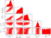 |
Fig. 2. Posterior probability distribution of the stellar population parameters of an example galaxy. The three different contour levels mark the 68%, 95%, and 99.7% enclosed probability regions. |
2.5. Weak-lensing data and cuts
We took weak lensing measurements from the first-year shape catalogue of the HSC survey (Mandelbaum et al. 2018). The source number density of this catalogue is 24.6 arcmin−2 (unweighted). Shapes are measured on coadded i−band images using the re-Gaussianization PSF correction method of Hirata & Seljak (2003). We refer to Mandelbaum et al. (2018) for details about the shape measurement process and the properties of the shape catalogue. We used photometric redshifts (photo-zs) obtained with the photo-z code MIZUKI (Tanaka 2015) on the data release 1 of the HSC survey (Tanaka et al. 2018).
The main weak-lensing analysis was carried out using the Bayesian hierarchical inference method of Sonnenfeld & Leauthaud (2018, SL18 from now on). This method is based on the isolated lens assumption: each lens galaxy in the sample is assumed to be at the centre of its dark matter halo, with no other mass component affecting the shape of the background sources around it. This assumption breaks down for satellite galaxies. It is therefore important to select a sample of lenses with the lowest possible satellite fraction. For this purpose, we first applied a cut in stellar mass, selecting only galaxies with observed stellar mass  , defined as the median of the posterior probability distribution in M*, larger than 1011 M⊙. Ninety percent of the CMASS galaxies left in our sample after the visual inspection step satisfied this requirement. We then matched our sample with the HSC cluster catalogue of Oguri et al. (2018), and removed objects with a cluster membership probability higher than 50% that were not identified as the brightest cluster galaxy. This step removed ∼5% of the objects in the sample.
Following the SL18 method, we modelled the weak-lensing signal produced by each lens on a set of background sources within a cone of a given radius, which we took to be 300 physical kpc at the redshift of the lens, where the isolated lens assumption is more realistic (i.e. where the so-called one−halo term dominates). One of the foundations of the SL18 method is the ability of treating the likelihood of the weak-lensing data around the lenses as independent of each other, which simplifies the problem greatly. However, when lenses lie in close proximity along the line of sight, the lensing cones of different lenses can overlap. In principle, we should simultaneously model the contribution of each lens on all the sources within the overlapping cones. In practice, this is computationally difficult. We avoided this problem by eliminating overlapping pairs using the same procedure adopted by SL18, which is as follows. We ranked the lenses in decreasing order of observed stellar mass, looped through them, and removed from the sample any lens whose cone overlapped with that of a more massive galaxy. The idea is that in case of lenses in close line-of-sight proximity, the main lensing signal should come from the most massive galaxy. Although in reality the problem is more complex (e.g. the strength of the lensing signal depends not only on the lens mass, but also on its redshift), the fraction of objects removed with this procedure is only 10%, and we do not expect this step to introduce any significant bias to our weak-lensing analysis (as has been shown by SL18 on mock observations). We then reached our final sample size of 10 403 CMASS galaxies.
To get a sense of the quality of the weak-lensing data available for our study, we carried out a stacked analysis. We made four bins in stellar mass and measured the stacked excess surface mass density ΔΣ in different radial bins using the HSC weak-lensing pipeline. We plot the ΔΣ profiles in Fig. 3. Differences in the lensing signal in different bins are detected with high confidence: this suggests that the data should allow us to determine not only an average halo mass of the sample, but also how halo mass scales with stellar mass, and possibly, with size. Figure 3 is only shown for illustration purposes: all our weak-lensing analysis was carried out by forward-modelling the weak-lensing signal of individual halos.
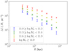 |
Fig. 3. Excess surface mass density profile in different bins of observed stellar mass, obtained by stacking the weak-lensing signal in circular annuli. |
2.6. Final sample
In Fig. 4 we plot the distribution in observed stellar mass, half-light radius, Sérsic index, and redshift of the final sample. The correlation between mass and size is very clear, as is a trend of increasing Sérsic index with stellar mass. In the next section we quantify the strength of these correlations.
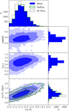 |
Fig. 4. Distribution in half-light radius, Sérsic index, and redshift as a function of stellar mass of the sample of 10 403 CMASS galaxies. Contour levels mark the 68%, 95%, and 99.7% enclosed probability regions. Blue contours and histograms refer to the fiducial model, consisting of a single Sérsic surface brightness profile for each galaxy. The distribution in stellar mass and size obtained with the SerExp model, described in Sect. 2.7, is plotted in green, while that obtained with the de Vaucouleurs model is marked by solid lines. |
Figure 5 shows the distribution of half-light radii in angular units. For most objects, the half-light radius is well within the 8.4″ region used for the fit, with only 1% of the galaxies in the sample exceeding this limit.
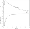 |
Fig. 5. Top panel: distribution in half-light radius, in angular units, of the galaxiese. Bottom panel: cumulative distribution in half-light radius. |
It is also interesting to check how far out from the centre of each galaxy the HSC data allow us to probe. For this purpose, we computed for each object the radius at which the best-fit i−band Sérsic surface brightness falls below the level of the root mean square fluctuation from the sky background, Rsky. We plot the distribution of Rsky/Re in Fig. 6. The median of this distribution is 3.6, with only 4% of the objects having a value of Rsky/Re lower than unity. For the typical galaxy in our sample, HSC i−band data then allow us to detect flux out to 3.6 times the half-light radius. For a de Vaucouleurs profile (n = 4, de Vaucouleurs 1948), the fraction of the total mass enclosed within this aperture is about 80%. This means that ∼20% (or 0.08 dex) of the total flux estimated for a typical galaxy is not directly observed, but rather the result of an extrapolation.
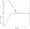 |
Fig. 6. Top panel: distribution in the ratio between the radius at which the i−band surface brightness of a galaxy falls below the sky fluctuation level, Rsky, and the half-light radius Re. Bottom panel: cumulative distribution. |
About 5% of the lenses are identified as brightest central galaxies (BCGs) in the HSC cluster catalogue of Oguri et al. (2018). For these objects, we expect intra-cluster light to contribute with a non-negligible fraction to the observed surface brightness. We did not attempt to separate the light of the central galaxy from the intra-cluster light, as the distinction between these two components is not very well defined. For cluster BCGs, our measurements of the surface brightness profile and the stellar mass and size derived from it must therefore be interpreted as that of the sum of the central galaxy and the intra-cluster light.
2.7. Alternative models
Our fiducial model for the surface brightness distribution of our galaxies consists of a single Sérsic component, as described in Sect. 2.3. In order to test for possible systematic effects related to this particular choice, we also considered two alternative models. The first of these models consists of a single de Vaucouleurs profile: it is a particular case of the more general Sérsic profile, and is known to provide a good description of the average surface brightness profile of local early-type galaxies. The second model is a two-component surface brightness profile, consisting of the sum of a Sérsic and an exponential profile (i.e. a Sérsic profile with n = 1). We imposed that the two components have the same centroid and colours, but allowed for different half-light radius, axis ratio, and position angle between the two. We refer to this as the “SerExp” model throughout this paper. The SerExp is a generalisation of the Sérsic model, and is expected to provide better fits because of the higher number of degrees of freedom. Bernardi et al. (2014) showed that a SerExp model provides a better description of the surface brightness profile of SDSS galaxies than models with a single Sérsic component.
In Fig. 7 we show the circularised i−band surface brightness profiles as well as the enclosed flux as a function of aperture for 20 example galaxies (the same objects as plotted in Fig. 1), obtained for the Sérsic, the de Vaucouleurs, and the SerExp model. In the region probed by HSC data, roughly where the galaxy is brighter than the sky fluctuation level (marked by the horizontal dashed line in each subplot), the differences between the Sérsic (blue curves) and the SerExp model (green curves) are very small. This is reassuring, as it means that the Sérsic model is sufficiently flexible to capture the complexity in the surface brightness profiles of our sample.
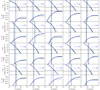 |
Fig. 7. i−band surface brightness profile (top sub-panel) and enclosed flux as a function of aperture (bottom sub-panel) for the best-fit Sérsic (blue), SerExp (green), and de Vaucouleurs (dotted black) profile for the 20 example objects shown in Fig. 1. The dashed horizontal line marks the surface brightness corresponding to the rms sky fluctuation. The dashed vertical lines mark the half-light radius. |
A similar case can be made for many objects for the de Vaucouleurs model, although for some systems the data clearly prefer Sérsic indices different from n = 4. These are the objects for which the best-fit de Vaucouleurs profile, shown as a dotted black curve, starts to deviate from the best-fit Sérsic profile well within the region above the background noise level. Typically, the residuals between the best-fit de Vaucouleurs profile and the data show under-subtraction at large radii for the systems with n > 4 and over-subtraction for the systems with n < 4.
The difference between the large R behaviour of the three models results in different total fluxes and, consequently, different half-light radii. For most of the objects in our sample, our data do not allow us to decide which of the three models is more accurate, especially between the Sérsic and the SerExp: the differences arise at large radii, where the surface brightness is too faint to be detected by HSC data. We therefore carried out the analysis with all models, and checked whether the results are stable with respect to the particular assumption on the large R behaviour of the surface brightness profile of our galaxies. Although the de Vaucouleurs model produces poor fits for a non-negligible fraction of the CMASS galaxies in our sample, we still show the results obtained with this particular surface brightness profile choice, since many studies in the literature are based on the same model.
3. Generalised mass-size relation
3.1. Basic model
We fitted for the mass-size relation of our sample of massive ( ) elliptical galaxies using a Bayesian hierarchical approach. We modelled the distribution of true stellar mass and size of the sample with a functional form, described by a set of hyper-parameters η, which we then inferred from the data. We chose the following form for this distribution:
 (4)
(4)
Here  is a skew Gaussian in log M*:
 (5)
(5)
with
 (6)
(6)
and  is a Gaussian in log Re
 (7)
(7)
with a mean that scales with stellar mass as follows:
 (8)
(8)
The hyper-parameters describing this 2D distribution are
 (9)
(9)
μ*, σ*, and s* describe the stellar mass distribution. If the skewness parameter s* is set to 0, this reduces to a Gaussian with mean μ* and dispersion σ*. Positive values of s* correspond to a distribution with a long tail above μ* and a sharper cutoff at low masses. The parameter μR, 0 is the average value of log Re at the pivot stellar mass log M* = 11.4, σ* is the scatter in log Re at fixed stellar mass, and finally, βR is a power-law dependence of Re on M*.
Our goal is to infer the posterior probability distribution of the set of hyper-parameters η given the data d. According to the Bayes’ theorem,
 (10)
(10)
where P(η) is the prior on the hyper-parameters and P(d|η) is the likelihood of observing the data given the value of the hyper-parameters. If measurements on separate galaxies are independent from each other, the latter is the following product over individual objects:
 (11)
(11)
In the above equation we have introduced a set of latent variables, the true values of the stellar mass and half-light radius of each galaxy. These are necessary to calculate the likelihood. We are not interested in constraining the stellar mass and size of individual galaxies, so we marginalised over all possible values, modulated by P(M*, i, Re, i|η), which is the distribution introduced in Eq. (4).
The data consist of the observed values of the stellar mass and the half-light radius,  and
and  , and related uncertainties. For simplicity, we neglected the uncertainty on size, since it is of the order of 2%. As a result, the covariance between the measurement of the half-light radius and the stellar mass was also set to zero. This is a fair approximation, since the uncertainty on the stellar mass is dominated by systematic uncertainties in the stellar population synthesis model. The first term in the integrand of Eq. (11) then becomes
 (12)
(12)
and Eq. (11) reduces to
 (13)
(13)
We approximated the likelihood of obtaining a value of the observed stellar mass  given the true value M*, i as a Gaussian in log M*, i:
 (14)
(14)
In the equation above, ϵ*, i is the standard deviation in log M*, i, as obtained from the MCMC chain of the stellar population fit, and Ai is a normalisation constant that ensures that the integral of the likelihood over all possible values of  is one. Since we applied the cut
  to define our sample, this is equivalent to
 (15)
(15)
We sampled the posterior probability distribution of the hyper-parameters η given the data d, Eq. (10), by running an MCMC. We calculated the integrals in Eq. (13) with the importance sampling and Monte Carlo integration method described in SL18. We assumed flat priors on all hyper-parameters except s*, for which we assumed a flat prior on its 10-base logarithm. In Fig. 8 we plot the posterior probability distribution relative to the parameters describing the distribution of sizes: μR, 0, σR and βR. The median and 68% credible interval of all hyper-parameters is reported in Table 1. We show results based on the Sérsic, SerExp, and de Vaucouleurs models.
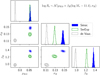 |
Fig. 8. Posterior probability distribution of the parameters describing the distribution of galaxy sizes as a function of stellar mass, introduced in Sect. 3.1. Results based on the Sérsic, SerExp, and de Vaucouleurs model are shown. |
We find a remarkably steep mass-size relation, although the exact value of the dependence of Re on M* depends on the choice of the photometric model: we obtain βR = 1.37 ± 0.01 when the Sérsic photometric model is used and βR = 1.22 ± 0.01 in the SerExp case. The difference between the models appears to be driven by differences in size at the high-mass end of the distribution: at fixed stellar mass, the values of Re obtained with the SerExp model are slightly lower than the Sérsic values, as can be seen from the bottom-left panel of Fig. 4. A similar behaviour was found by Bernardi et al. (2014) on SDSS galaxies. As a result, the uncertainty on our inference on the slope of the mass-size relation is dominated by systematics related to the particular choice of the surface brightness profile used to describe CMASS galaxies.
The difference between the Sérsic and the de Vaucouleurs sizes is much more evident, hence the much lower value of the mass-size relation slope inferred for this particular model: βR = 0.98 ± 0.01. However, we believe this to be a biased inference, since a de Vaucouleurs model provides a poor description of the surface brightness profile of a non-negligible fraction of the objects in our sample.
3.2. Distribution of size and Sérsic index
We added complexity to our model by considering the distribution in Sérsic index of our galaxies, in addition to stellar mass and size. We modelled the distribution in M*, n and Re as follows:
 (16)
(16)
The term  is the same as introduced in Eqs. (5) and (6).
  is a Gaussian distribution in the base-10 logarithm of the Sérsic index,
 (17)
(17)
with a mean that scales with stellar mass as
 (18)
(18)
and dispersion σn. Finally, we kept the same form as Eq. (7) for the term describing the distribution in half-light radius,  , but updated Eq. (8) by adding a dependence on the Sérsic index to the average size:
 (19)
(19)
At fixed stellar mass, Eq. (16) is a bi-variate Gaussian in log n and log Re.
As we have done for the sizes, we assumed that the Sérsic indices are measured exactly, since the uncertainties on n are very small. In Fig. 9 we plot the posterior probability distribution of the hyper-parameters describing the distribution in Sérsic index, μn, 0, σn, and βn, as well as the hyper-parameters describing the distribution in size, including the new hyper-parameter νR, which describes the dependence of size on n. The median and 68% credible values of all hyper-parameters are listed in Table 2. We show only the result based on the Sérsic model, as n is not well defined in the case of a SerExp profile and is fixed in the case of a de Vaucouleurs model.
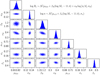 |
Fig. 9. Posterior probability distribution of the parameters describing the distribution of Sérsic index and galaxy size. |
The inferred average value of log n at the pivot stellar mass log M* = 11.4 is μn, 0 = 0.704 ± 0.002, corresponding to a Sérsic index n ≈ 5.1. We find a positive correlation between Sérsic index and stellar mass, quantified by the parameter βn = 0.464 ± 0.009. This is closely related to the well-known Sérsic index - luminosity correlation (Caon et al. 1993), and tells us that, for instance, the average Sérsic index of galaxies with stellar mass log M* = 11.8 is as high as n ≈ 7.8. We also find a correlation between size and Sérsic index at fixed stellar mass: νR = 0.38 ± 0.01.
The value of parameter βR, the correlation between mass and size, is lower than the value obtained in the analysis of Sect. 3.1, based on the simpler model (1.18 vs 1.37). This is because in the context of this more complex model, βR quantifies how size scales with stellar mass at fixed Sérsic index. The combination of this scaling with 1) the dependence of size on n (positive value of parameter νR) and 2) the positive correlation between Sérsic index and stellar mass produces the steep mass-size relation observed.
At the same time, the inferred value for the average size at the pivot point, μR, 0, is lower than the value obtained previously. This is because μR, 0 now refers to the average log Re at a stellar mass log M* = 11.4, and Sérsic index n = 4, corresponding to a de Vaucouleurs profile, which is a lower value of n than the average for galaxies of that mass.
The high Sérsic indices measured in this study provide a good description of the surface brightness profile of CMASS galaxies in the region probed by the data, which roughly corresponds to the radial range 2 kpc ≲ R ≲ 30 kpc. The lower limit is set by the finite resolution of HSC data. An extrapolation of the best-fit Sérsic profile to the very inner regions produces very steep inner surface brightness profiles. Such cuspy profiles are typically not observed in the centres of nearby massive galaxies, but cannot be ruled out in our observations because of the atmospheric blurring of the images. The impact of a potentially inaccurate description of the inner surface brightness profile on the stellar mass and size measurement used for our study is nevertheless very low: the mass enclosed in the region that is significantly affected by the atmospheric seeing is only a small fraction of the total. However, we urge caution when using our derived Sérsic fits to predict quantities that are more sensitive to the inner stellar distribution, such as the dynamical mass.
The outer limit to the region where the Sérsic profile is most accurate is set by the radius at which the surface brightness of CMASS galaxies falls below the noise level of HSC data. The median value of this radius for our sample is 28 kpc.
4. Generalised stellar-to-halo mass relation
We now use weak-lensing measurements from HSC to obtain the dark matter halo mass distribution of our sample as a function of galaxy properties. We explore two different models with increasing degrees of complexity. In the first model, presented in the next subsection, we let the halo mass scale with stellar mass and half-light radius. In Sect. 4.2, we generalise this model to allow for a possible additional dependence of halo mass on Sérsic index.
Mirroring the approach adopted in Sect. 3, we fit the simpler of the two models to data obtained with the three different parameterisations of the surface brightness profiles in order to explore the impact of potential systematics associated with the photometry fitting on the derived stellar-to-halo mass relation. We then fit the full model to our fiducial Sérsic profile-based measurements.
4.1. Halo mass as a function of stellar mass and size
We start by considering the joint distribution in stellar mass M*, half-light radius Re and halo mass Mh. Similarly to the approach adopted in the previous Section, we modelled this distribution as follows:
 (20)
(20)
The terms  and
and  are the same as introduced in Sect. 3.1: a skew Gaussian in log M* and a Gaussian in log Re with a mean that scales with stellar mass. The term relative to the halo mass,
  , is modelled as a Gaussian in log Mh,
 (21)
(21)
with a mean that scales with stellar mass and size as
 (22)
(22)
and dispersion σh. The term μR(M*) in Eq. (22) is the average log Re for galaxies of mass M*, introduced in Eq. (8). The parameter ξh is then a power-law dependence of halo mass on “excess size”, defined as the ratio between the half-light radius of a galaxy and the average size for galaxies of the same stellar mass. This excess size is conceptually similar to the “mass-normalised radius” used by Newman et al. (2012) and Huertas-Company et al. (2013b).
The full list of hyper-parameters of the model is then
 (23)
(23)
In order to infer the posterior probability distribution of the hyper-parameters given the data, we need to be able to evaluate the likelihood P(d|η) for any value of η. Under the isolated lens assumption on which the S18 weak-lensing method is based, the likelihood of the data relative to each lens is independent of each other. We can then write, analogously to Eq. (11),
 (24)
(24)
For each galaxy, the data consist of the measured stellar mass, effective radius, and shape measurements of background sources within a cone of 300 physical kpc radius at the redshift of the lens (as previously discussed in Sect. 2.5). In order to evaluate the likelihood of the shape measurements, it is necessary to assume a model for the mass distribution of the lens. We first defined the halo mass as the dark matter mass enclosed in a shell with average density equal to 200 times the critical density of the Universe, commonly referred to as M200. We then assumed a spherical Navarro-Frenk-White (NFW, Navarro et al. 1997) shape for the dark matter halo density profile:
 (25)
(25)
Finally, we assumed the mass-concentration relation from Macciò et al. (2008): given r200 (the radius enclosing a mass equal to M200), we assumed that the concentration ch = r200/rs is drawn from the following Gaussian in its base-10 logarithm:
 (26)
(26)
with a mean μc that scales with halo mass as
 (27)
(27)
and dispersion σc. We fix μc, 0 = 0.830, βc = −0.098 and σc = 0.10.
For each galaxy, the likelihood of observing the data given the value of the hyper-parameters is obtained by marginalising over all possible values of the concentration, as well as stellar and halo mass and half-light radius:
 (28)
(28)
Here P(ch, i|Mh, i) is the mass-concentration relation introduced in Eq. (26), which acts as a prior on the concentration parameter. As done throughout Sect. 3, we set the uncertainty on the half-light radius to zero so that the integral over Re reduces to that over a delta function. The likelihood of the weak-lensing data is obtained by evaluating the shear produced by the lens, given the values of M*, Mh, and ch, corrected for by an additive and multiplicative bias on the measurements, obtained through simulations by Mandelbaum et al. (2018). We refer to SL18 and Sonnenfeld et al. (2018, Sect. 3.4) for more details on the calculation of the likelihood term for weak-lensing data in the SL18 formalism.
In Fig. 10 we plot the posterior probability distribution of the hyper-parameters belonging to the halo mass term  in Eq. (20). The median and 68% credible interval on the full set of hyper-parameters is given in Table 3. We show results based on the Sérsic, SerExp, and de Vaucouleurs model.
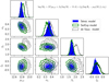 |
Fig. 10. Posterior probability distribution of the parameters describing the distribution of halo mass for the model introduced in Sect. 4.1. In particular, μh, 0 is the average log Mh at a stellar mass log M* = 11.4 and average size for that mass, σh is the dispersion in log Mh around the average, βh is a power-law scaling of halo mass with stellar mass, and ξh is a power-law scaling of halo mass with excess size (defined as the ratio between the size of a galaxy and the average size of galaxies of the same stellar mass). |
The average log Mh for galaxies of log M* = 11.4 and average size for their mass is μh, 0 = 12.79 ± 0.03. We then infer a positive correlation between halo mass and stellar mass at fixed size, βh = 1.70 ± 0.10. However, we fail to find any strong evidence for an additional correlation between halo mass and size at fixed stellar mass. The median and 1σ limit of the parameter describing the dependence on size is ξh = −0.14 ± 0.17, consistent with zero.
These values were obtained using sizes and stellar masses based on the Sérsic photometric model, but the SerExp model produced consistent results, as we show in Fig. 10. The main differences are that the SerExp model produces a steeper halo mass-stellar mass relation (higher value of parameter βh), and that the inference on the halo mass-size correlation is broader and closer to zero (ξh = −0.03 ± 0.21). The broadening of the posterior probability distribution on parameter ξh is related to the smaller intrinsic scatter around the stellar mass-size relation measured for the SerExp model (σR = 0.13 vs. σR = 0.15 obtained using Sérsic): a smaller intrinsic scatter means a shorter lever arm in the measurement of the secondary correlation between Mh and Re at fixed M*, which in turn results in lower precision.
Using the photometric measurements obtained by imposing a de Vaucouleurs profile, we obtain an even steeper stellar-to-halo mass relation, βh = 2.04 ± 0.15, and an average halo mass at the pivot stellar mass (parameter μh, 0) ∼0.1 dex higher than the Sérsic case. This difference is related to the different stellar mass distributions obtained with the two models: a de Vaucouleurs profile tends to under-estimate the stellar mass of the most massive CMASS galaxies, for which the data favour values of the Sérsic index n > 4. This flattening in the slope of the stellar-to-halo mass relation β when going from a de Vaucouleurs to a Sérsic model is a well-known effect (see e.g. Shankar et al. 2014b, 2018; Kravtsov et al. 2018).
In our model of the generalised stellar-to-halo mass relation, stellar mass and size are treated as the independent variables, while halo mass is the dependent variable. For the purpose of comparing our results with other studies, it can be useful to invert this relation and obtain the distribution of size as a function of halo mass. This can be done with a posterior predictive procedure: we fixed the value of the stellar mass to log M* = 11.4, drew samples of the hyper-parameters from the posterior probability distribution, and for each value of the hyper-parameters, then drew samples of halo mass and half-light radius for the corresponding model. In Fig. 11 we plot the resulting distribution of Re as a function of Mh. This can be interpreted as our inference of the size-halo mass distribution of log M* = 11.4 galaxies, assuming our sample is complete in size at this value of the stellar mass.
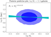 |
Fig. 11. Posterior predictive distribution in half-light radius as a function of halo mass for galaxies with log M* = 11.4. This is obtained by first drawing values of the hyper-parameters from the posterior probability distribution of our Sérsic model-based inference, then drawing values of Re and Mh for 1000 galaxies, given the model specified by the hyper-parameters. Blue contours correspond to 68% and 95% enclosed probability. The cyan band shows the 68% credible region of the size-halo mass relation, obtained by fitting a power-law relation to the mock distribution of Re and Mh at each draw of the hyper-parameters. |
We can then summarise this distribution by fitting a power-law halo mass-size relation to it. We performed this for each draw of the values of the hyper-parameters, obtaining  , corresponding to the cyan band in Fig. 11. This is an alternative visualisation of our main result, consisting of a lack of a strong correlation between halo mass and size at fixed stellar mass.
4.2. Halo mass as a function of stellar mass, Sérsic index, and size
We now add a dimension to our model: the Sérsic index. We modified the galaxy probability distribution Eq. (20) by adding a term describing the distribution in n as follows:
 (29)
(29)
The term  is the same introduced in Eq. (17): a Gaussian in the base-10 logarithm of the Sérsic index, with a mean that scales with stellar mass, as parameterised in Eq. (18). Then, as done in Sect. 3.2, we let the mean of the size distribution scale with Sérsic index, according to Eq. (19). Finally, we modified the mean of the Gaussian distribution in log Mh to allow for a power-law dependence of halo mass on Sérsic index as follows:
 (30)
(30)
In the above equation, μn(M*) is the average base-10 logarithm of the Sérsic index for galaxies of mass M*, defined in Eq. (18). The new parameter νh describes how halo mass scales with “excess Sérsic index”: the ratio between the value of n of a galaxy and the typical value of n for galaxies of the same stellar mass.
The motivation for allowing the halo mass to vary with Sérsic index is the following: different values of n for galaxies of the same stellar mass point to different evolutionary histories, possibly related to the number and type of mergers experienced. If differences in evolutionary paths are reflected in the halo mass, we should be able to detect a correlation between n and Mh.
We ran an MCMC to sample the posterior probability distribution of the Sérsic profile-based model, given the data. The inference on the hyper-parameters describing the halo mass distribution is shown in Fig. 12, while the median values and 68% credible regions of the inference on all the model hyper-parameters are listed in Table 4.
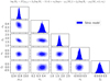 |
Fig. 12. Posterior probability distribution of the parameters describing the distribution of halo mass for the model including a dependence of Mh on the Sérsic index introduced in Sect. 4.2. In particular, μh, 0 is the average log Mh at a stellar mass log M* = 11.4, average n for that mass and average size given M* and n. σh is the dispersion in log Mh around the average, βh is a power-law scaling of halo mass with stellar mass, νh is a power-law scaling of halo mass with excess Sérsic index (defined as the ratio between the Sérsic index of a galaxy and the average n of galaxies of the same stellar mass), and ξh is a power-law scaling of halo mass with excess size. |
Median values and 68% credible interval of the posterior probability distribution of the hyper-parameters describing the distribution in stellar mass, half-light radius, Sérsic index, and halo mass of the galaxies in our sample, as inferred by fitting the model introduced in Sect. 4.2 to the Sérsic profile-based measurements.
The results change little with respect to the inference based on the simpler model used in the previous subsection. Most notably, the inference on the new parameter νh, describing the correlation between halo mass and Sérsic index, is consistent with zero: νh = −0.11 ± 0.14. Our data therefore allow us to rule out any strong dependence of halo mass on Sérsic index.
5. Discussion
5.1. Role of observational scatter
The main result of our study is the measurement of the correlation, or lack thereof, between halo mass and galaxy size at fixed stellar mass. This is a non-trivial measurement to make: galaxies are distributed along a relatively narrow mass-size relation, with a 0.15 dex intrinsic scatter in Re at fixed M*, meaning that any such signal is to be searched for across a small dynamic range in size. Additionally, observational errors cause data points to move in the M* − Re plane from their true position. If not modelled, these errors can introduce biases: for instance, at fixed observed stellar mass, larger size galaxies are on average more massive than their smaller size counterparts, making the interpretation of correlations measured directly on point estimates of observed quantities problematic (see Sect. 2.2 of SL18 for a more detailed explanation).
The Bayesian hierarchical formalism on which this study is based allows us to forward-model the effects of observational scatter and thus obtain an unbiased measurement of the true distribution of the model parameters, provided that the estimates of the observational uncertainties are accurate.
We obtained uncertainties on the values of M* by fitting stellar population synthesis models to HSC photometric data, adding a 0.05 mag systematic uncertainty to the magnitudes to account for the typical mismatch between the best-fit model and the data to avoid unrealistically small errors (see Sect. 2.4). As a result, the derived uncertainty on M* is to some extent arbitrary, as it reflects our choice on the amplitude of the systematic error added to the data. Moreover, the error on M* is also set by the priors on the stellar population parameters entering the fit, such as age or dust attenuation.
The median value of the uncertainty on M* of the sample is 0.10 dex. In order to test the impact of making a more conservative choice on the estimate of the stellar mass uncertainty, we repeated the analysis of Sect. 4.1 after adding in quadrature a further 0.10 dex systematic error on M*. The inference on the hyper-parameters describing the distribution in halo mass is plotted in red in Fig. 13 on top of the original inference (in blue). For the sake of simplicity, we only show results based on the Sérsic model. The inference on the halo mass-size correlation parameter ξh changes: with the larger observational uncertainties on M*, high negative values of ξh are allowed by the data. However, strong positive correlations between Mh and Re are still ruled out even with inflated error bars on M*.
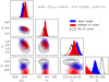 |
Fig. 13. Posterior probability distribution of the parameters describing the distribution of halo mass based on the model of Sect. 4.1. The blue contours show the inference obtained using the Sérsic model, as obtained in Sect. 4 and plotted in Fig. 10. The distribution shown in red has been obtained by repeating the analysis of the Sérsic model and adding 0.1 dex in quadrature to the uncertainties on the observed stellar masses. The solid lines mark the distribution obtained by setting all uncertainties on the stellar masses to zero. |
For the sake of completeness, we also show the results obtained by setting the uncertainties on M* to zero (solid lines in Fig. 13). In this case, the data seem to favour a positive correlation between halo mass and size. However, as discussed by SL18, this is a biased inference.
5.2. Comparison with other observational studies
5.2.1. Mass-size relation
A striking result of our study is the steep stellar mass-size relation: as shown in Sect. 3.1, we find  when a single Sérsic model is used to describe the surface brightness profile of CMASS galaxies (
 for the SerExp model). By comparison, most studies of the mass-size relation in quiescent galaxies find much shallower slopes, with βR ≈ 0.5 − 0.6 (see e.g. van der Wel et al. 2008; Damjanov et al. 2011; Newman et al. 2012; Huertas-Company et al. 2013b). The main reason for this discrepancy probably lies in the stellar mass distribution of our sample. The median stellar mass is log M* = 11.45, higher than that of the samples used in the aforementioned studies. As shown by Bernardi et al. (2011), the mass-size relation is not a strict power-law at all masses, but becomes steeper above M* ∼ 2 × 10¹¹, where most of the galaxies in our sample lie. We are then probing a region of parameter space where the slope of the M* − Re relation is steeper than the value that characterises quiescent galaxies at lower masses.
It is more difficult to reconcile our results with the study of Favole et al. (2018): in their analysis of the mass-size relation of CMASS galaxies, they find a slope βR ≈ 0.2, much shallower than our result, and also shallower than other studies on different samples of quiescent galaxies, such as those mentioned above. Favole et al. (2018) used de Vaucouleurs profiles to describe early-type galaxies in the CMASS sample: their measurement should therefore be compared with the value of the mass-size slope we inferred for the same surface brightness profile assumption: βR = 0.98.
A key difference in the Favole et al. (2018) study is in the stellar mass measurements: while we fitted stellar population synthesis models to HSC photometry, they used stellar masses from the Portsmouth stellar mass catalogue (Maraston et al. 2013). The Portsmouth stellar masses are obtained from SDSS photometry, which are much noisier than HSC data. This could lead to a higher observational scatter that would flatten the observed M* − Re relation if it is not accounted for.
5.2.2. Stellar-to-halo mass relation
The stellar-to-halo mass relation of CMASS galaxies was studied by Tinker et al. (2017) using galaxy clustering and abundance matching and taking advantage of the stellar mass completeness study of Leauthaud et al. (2016). In Fig. 14 we plot the average value of log Mh as a function of log M* as measured by Tinker et al. (2017) on top of the same quantity obtained from our inference, calculated using Eq. (22). The stellar masses used by Tinker et al. (2017) were obtained under the assumption of a Kroupa initial mass function (IMF), which we converted into Chabrier IMF-based stellar masses by applying a −0.05 dex shift.
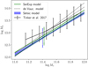 |
Fig. 14. Average value of log Mh as a function of M*. The blue band and the green and dotted black pairs of lines show the 1σ confidence limit obtained from our analysis based on the Sérsic, SerExp, and de Vaucouleurs model, respectively. The solid black line is a measurement from Tinker et al. (2017), obtained from galaxy clustering and abundance matching. Error bars indicate the intrinsic scatter in log Mh. The inner (outer) ticks on the error bars relative to our measurements refer to the 84 (16) percentile of our inference on the scatter parameter σh. The inference on the intrinsic scatter obtained with the de Vaucouleurs model is omitted to avoid confusion. |
The clustering-based measurement of Tinker et al. (2017) is systematically above our Sérsic profile-based results by ∼0.2 − 0.3 dex. This discrepancy is similar to the one observed by Leauthaud et al. (2017) in their comparison between the clustering and stacked weak-lensing signal of the CMASS sample. Leauthaud et al. (2017) discussed various possible ways to solve this tension, including varying the value of the cosmological parameter  , allowing for baryonic physics effects or assembly bias in the models used to map the clustering to the weak-lensing signal, allowing for the presence of massive neutrinos or deviations from general relativity. Part of the difference could also be due to the different photometric data and surface brightness profile used for the stellar mass measurements on which the Tinker et al. (2017) study is based: they used cmodel magnitudes obtained from SDSS, while we are showing results based on Sérsic and SerExp fits on much deeper HSC data. As Fig. 14 shows, using a more restrictive de Vaucouleurs profile, which is typically the dominant component in cmodel fits of massive quiescent galaxies, leads to a much better agreement in the average halo mass.
Given all these potential systematics affecting the comparison between clustering and lensing, the discrepancy between our measurement and the Tinker et al. (2017) study is not particularly worrisome. We point out the very good agreement on the inference on both the slope of the stellar-to-halo mass relation and the intrinsic scatter between the two measurements.
5.2.3. Correlation between galaxy size and halo mass
Many studies have examined the correlation between galaxy sizes and the environment they live in at fixed stellar mass, with somewhat conflicting results (see Sect. 1). Among these studies, the work by Huang et al. (2018a) is particularly relevant for our analysis, since it is based on a sample of massive galaxies with photometric data from the HSC survey, selected for having a stellar mass enclosed within a radius of 100 kpc higher than 1011.6 M⊙ and a spectroscopic redshift in the range 0.3 < z < 0.5. A good fraction of the galaxies in the Huang et al. (2018a) sample also belong to our sample of CMASS galaxies.
Huang et al. (2018a) showed that at fixed value of the stellar mass within 100 kpc in projection, M*, 100 kpc, galaxies that are identified as the central of a massive cluster (log Mh ≳ 14) have preferentially lower values of the stellar mass enclosed within 10 kpc, M*, 10 kpc. Using M*, 100 kpc as the fiducial value of the stellar mass of a galaxy, this result can be interpreted as the evidence for more extended galaxies (lower value of M*, 10 kpc at fixed M*, 100 kpc) living preferentially in more massive halos. A recent stacked weak-lensing analysis of the same set of objects confirmed the result (Huang et al. 2018b).
We wish to test whether this trend can be seen in our data as well. For this purpose, we performed a posterior predictive test: we used our model to generate mock data, and checked whether this mock data reproduces the trend observed by Huang et al. (2018a). We proceeded as follows: we took the maximum-likelihood values of the hyper-parameters describing the distribution in stellar mass, Sérsic index, and size, as measured in Sect. 3.2, as well as the hyper-parameters describing the distribution in halo mass, as inferred in Sect. 4 for the Sérsic case. For the sake of a more straightforward interpretation of the results, we set the value of the correlation between halo mass and size to zero, ξh = 0, which is consistent with our inference. We drew a large set of values of M*, n, Re, Mh, then computed the corresponding values of M*, 100 kpc and M*, 10 kpc for each object.
Both our predicted M*, 100 kpc and M* are model-dependent quantities: we only used data within 8.4″ to constrain the surface brightness profile of our galaxies, corresponding to a projected physical aperture of 54 kpc at a redshift z ∼ 0.55. We then extrapolated the Sérsic profile to obtain values of M*, 100 kpc and M*.
In the bottom panel of Fig. 15 we plot the values of M*, 10 kpc as a function of M*, 100 kpc. As done in Fig. 9 of Huang et al. (2018a), we selected objects with log M*, 100 kpc > 11.6, split the sample between galaxies that lie in halos more massive than log Mh = 14 (in red) and less massive (in grey), then fit the M*, 10 kpc − M*, 100 kpc distribution of each subsample with a linear relation.
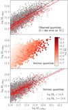 |
Fig. 15. Posterior predictive plot, showing the stellar mass enclosed within 10 kpc as a function of the stellar mass enclosed within 100 kpc of a mock sample of galaxies, generated from the maximum-likelihood values of the hyper-parameters of our single Sérsic profile-based model. Bottom panel: sample split between galaxies that live in halos more massive than 1014 M⊙ (red squares) and those that live in less massive halos (grey dots). The red and black lines are the best-fit linear relations between M*, 10 kpc and M*, 100 kpc for the more massive halos and less massive halos, respectively. Middle panel: data points from the bottom panel are colour-coded according to the total stellar mass. Top panel: same as the bottom panel, but with a 0.1 dex random error on the stellar mass measurements. |
Qualitatively, we see a similar trend to that reported by Huang et al. (2018a): at fixed M*, 100 kpc, galaxies at the centre of massive halos have preferentially lower values of M*, 10 kpc. This might seem to contradict the way our model was built, since we removed any dependence of the halo mass on size at fixed stellar mass. However, in the context of the Sérsic models at the basis of our analysis, a non-negligible fraction of the total stellar mass of a galaxy comes from stars located beyond 100 kpc in projection, especially for very massive galaxies like those considered in this experiment. The fraction of stellar mass beyond 100 kpc is larger for galaxies with larger sizes: this implies that at fixed M*, 100 kpc, galaxies with larger sizes or with lower values of M*, 10 kpc are on average more massive (have a higher value of M*). As a result, these galaxies tend to live in more massive dark matter halos on average. This can verified in the middle panel of Fig. 15, where the same data points of the plot in the bottom panel are colour-coded by the total stellar mass of each object: stellar mass increases with increasing M*, 100 kpc, but also with decreasing M*, 10 kpc. Halo mass follows a similar trend.
In the top panel of Fig. 15 we show a version of the bottom plot of the same figure, modified by adding a 0.1 dex random observational scatter on the stellar mass measurements. This observational scatter is meant to simulate errors in the stellar population synthesis fitting, therefore they affect the measurements of the stellar mass at different radii in the same way (i.e. they shift the values of log M*, 100 kpc and log M*, 10 kpc by exactly the same amount). The difference in the M*, 10 kpc − M*, 100 kpc relation between clusters and lower-mass halos increases when we consider the observed quantities, and is similar in amplitude to the signal measured by Huang et al. (2018a). This is related to the distortion of the mass-size relation due to observational scatter discussed in Sect. 5.1 and can be understood as follows: given a bin in observed stellar mass, smaller sized galaxies are statistically more likely to have scattered into the bin from lower intrinsic stellar masses than larger sized galaxies (see also Sect. 2.2 of SL18).
Both of the effects discussed above follow simply from the existence of a positive correlation between stellar mass and size and do not depend on a particular form of the mass-size or mass-Sérsic index relation. We have verified that making the same posterior predictive plot based on de Vaucouleurs fits produces very similar results.
After this test, we conclude that our inference is consistent with the Huang et al. (2018a) analysis. In the context of our model, the correlation between halo mass and the observed values of M*, 10 kpc at fixed M*, 100 kpc can be explained with the combination of two causes: massive galaxies having a non-negligible fraction of their stellar mass beyond 100 kpc, and the effect of observational scatter on the stellar mass measurements.
Charlton et al. (2017) measured the correlation between halo mass and galaxy size at fixed stellar mass using stacked weak-lensing measurements in a large set of galaxies. Charlton et al. (2017) made bins in luminosity and size and studied the variation in halo mass, as measured from weak lensing, as a function of size after accounting for the dependence of halo mass on stellar mass. They measured a value ξh = 0.42 ± 0.12, which is inconsistent with our inference. SL18 argued that part of their signal could be due to the effects of observational scatter. This would definitely be the case if their stacked weak-lensing analysis was carried out in bins of observed stellar mass: as Fig. 13 shows, ignoring observational errors on M* can introduce a signal of similar magnitude to the reported value. However, Charlton et al. (2017) carried our their analysis in luminosity bins. Luminosity is measured with a much greater accuracy than stellar mass, and this should lead to a more accurate inference on the parameter ξh. Nevertheless, the Charlton et al. (2017) analysis still relies on noisy stellar mass measurements from stellar population synthesis modelling, and this should have some impact on the inference, if not taken into account. For a fair comparison, it would be important to test the effects of observational scatter in a study of the halo mass-size correlation à la Charlton et al. (2017). This is beyond the scope of this paper, however.
5.3. Comparison with theoretical models
The relation between halo mass and galaxy size has been investigated in theoretical works based on both semi-analytical models or hydrodynamical simulations. Shankar et al. (2014a) explored various different semi-analytical models, finding that most of these models predict a positive correlation between halo mass and size at fixed stellar mass. They showed that such a correlation can emerge simply as the result of dissipationless mergers: although the major merger rate is a very mild function of halo mass, the rate of minor mergers can be higher in higher-mass halos if the merging timescale, which is set by dynamical friction, is sufficiently short. For a given increase in stellar mass, minor mergers produce a higher increase in size than major mergers (Naab et al. 2009; Hopkins et al. 2010a): if minor mergers are more frequent in more massive halos, then this can introduce a halo mass-size correlation at fixed stellar mass. Whether this effect is real, however, depends on the merging timescale and its dependence on the mass of the central halo and that of the accreted object, which is very difficult to determine observationally (see also Hopkins et al. 2010b; Nipoti et al. 2012, for related discussions on merger timescales and the effects of mergers on the size evolution of massive galaxies). With the dynamical friction timescales from McCavana et al. (2012), the semi-empirical hierarchical growth model of Shankar et al. (2015) found only a mild dependence on halo mass in the size growth of massive galaxies.
Other processes that can produce a positive correlation between halo mass and size at fixed stellar mass are disc instabilities, gas dissipation in major mergers, and the differential evolution of accreted galaxies in low- and high-mass halos. We refer to Shankar et al. (2014a) for details on these mechanisms. Shankar et al. (2014a) claimed that models predicting a significant correlation between halo mass and galaxy size are disfavoured by observational data and based this on evidence from Huertas-Company et al. (2013a). Our analysis further strengthens their point.
We also point out that although we focused our comparison on theoretical models that are based on a merger-driven size growth scenario, it is possible that the most massive galaxies observed at z < 1 have assembled most of their mass through in situ processes during their early evolutionary phases (see Buchan & Shankar 2016, for a related discussion). In this case, it is not clear if a correlation between size (or Sérsic index) and halo mass at fixed stellar mass is expected at all.
Charlton et al. (2017) examined the halo mass-size correlation at fixed M* in the EAGLE (Schaye et al. 2015) and ILLUSTRIS samples (Vogelsberger et al. 2014). They found values of ξh in the range 0.5 ≲ ξh ≲ 1.0 at the stellar masses probed by our study, although they found lower values when their measurement was restricted to central galaxies. For instance, they reported a value of ξh = 0.29 ± 0.23 for EAGLE galaxies in a bin of median stellar mass log M* = 11.34 when satellites were excluded. A similar value (ξh = 0.18 ± 0.07) was measured by Desmond et al. (2017) in the same simulation. Our measurements are in agreement with these values to within 2σ, therefore we do not register a great difference between predictions from hydrodynamical simulations and our data.
6. Conclusions
We used HSC imaging and weak-lensing measurements for a set of ∼10 000 galaxies from the CMASS sample to constrain 1) the stellar mass-size relation, 2) the stellar mass-Sérsic index-size relation, 3) the stellar mass-size-halo mass relation, and 4) the stellar mass-size-Sérsic index-halo mass relation of massive (log M* > 11) galaxies at redshift z ∼ 0.55. We found the following:
-
The stellar mass-size relation at the high mass end is very steep: modelling this as a power law,
 , we find values of βR higher than unity, with the actual value depending on the choice of surface brightness profile used to fit the photometry.
 -
The average Sérsic index of our sample increases with increasing stellar mass as
 . At fixed stellar mass, size correlates positively with Sérsic index.
 -
Halo mass scales with the ∼1.7 power of stellar mass. At fixed stellar mass, we find no evidence for an additional correlation of halo mass with size or Sérsic index. As a consequence, our measurement disfavours models of galaxy evolution in which galaxy size grows more efficiently in high-mass halos than in low-mass halos.
-
The halo masses of the CMASS sample inferred from weak lensing are on average 0.2 − 0.3 dex lower than those inferred from galaxy clustering, although much of this discrepancy could be due to differences in the photometric data and the choice of the surface brightness profile used to model galaxies, on which stellar mass measurements are based.
The observational data at the core of this work is the weak-lensing measurements from HSC. These data consist of observations carried out in the first year of the survey, covering ∼140 deg2. As the HSC survey reaches completion, similar quality measurements over a much larger area will soon be available. This should allow us to reduce statistical uncertainties on the distribution of halo masses. However, for the key parameter subject of this study, the correlation between halo mass and size at fixed stellar mass ξh, the inferred value depends in a non-negligible way on the surface brightness profile used to fit the photometric data, on which the stellar mass and size measurements are based. As statistical errors shrink, the systematic effect connected to this aspect of the model will start to dominate. We point out that as shown in Sect. 2.7, most of the difference between the measurements based on the Sérsic and SerExp models is due to the extrapolation of the surface brightness profile at large radii, where the model is unconstrained by the data. We therefore expect that the next challenge in determining the correlations between the stellar distribution in galaxies and their host dark matter halos will be measuring the light profile in the very outskirts of galaxies.
Acknowledgments
AS acknowledges funding from the European Union’s Horizon 2020 research and innovation programme under grant agreement No 792916, as well as a KAKENHI Grant from the Japan Society for the Promotion of Science, MEXT, No JP17K14250. This work was supported by World Premier International Research Center Initiative (WPI Initiative), MEXT, Japan. The Hyper Suprime-Cam (HSC) collaboration includes the astronomical communities of Japan and Taiwan, and Princeton University. The HSC instrumentation and software were developed by the National Astronomical Observatory of Japan (NAOJ), the Kavli Institute for the Physics and Mathematics of the Universe (Kavli IPMU), the University of Tokyo, the High Energy Accelerator Research Organization (KEK), the Academia Sinica Institute for Astronomy and Astrophysics in Taiwan (ASIAA), and Princeton University. Funding was contributed by the FIRST program from Japanese Cabinet Office, the Ministry of Education, Culture, Sports, Science and Technology (MEXT), the Japan Society for the Promotion of Science (JSPS), Japan Science and Technology Agency (JST), the Toray Science Foundation, NAOJ, Kavli IPMU, KEK, ASIAA, and Princeton University. Funding for SDSS-III has been provided by the Alfred P. Sloan Foundation, the Participating Institutions, the National Science Foundation, and the US Department of Energy Office of Science. The SDSS-III web site is http://www.sdss3.org/. SDSS-III is managed by the Astrophysical Research Consortium for the Participating Institutions of the SDSS-III Collaboration including the University of Arizona, the Brazilian Participation Group, Brookhaven National Laboratory, Carnegie Mellon University, University of Florida, the French Participation Group, the German Participation Group, Harvard University, the Instituto de Astrofisica de Canarias, the Michigan State/Notre Dame/JINA Participation Group, Johns Hopkins University, Lawrence Berkeley National Laboratory, Max Planck Institute for Astrophysics, Max Planck Institute for Extraterrestrial Physics, New Mexico State University, New York University, Ohio State University, Pennsylvania State University, University of Portsmouth, Princeton University, the Spanish Participation Group, University of Tokyo, University of Utah, Vanderbilt University, University of Virginia, University of Washington, and Yale University.
References
- Aihara, H., Arimoto, N., Armstrong, R., et al. 2018a, PASJ, 70, S4 [NASA ADS] [Google Scholar]
- Aihara, H., Armstrong, R., Bickerton, S., et al. 2018b, PASJ, 70, S8 [NASA ADS] [Google Scholar]
- Allen, R. J., Kacprzak, G. G., Spitler, L. R., et al. 2015, ApJ, 806, 3 [NASA ADS] [CrossRef] [Google Scholar]
- Anderson, L., Aubourg, É., Bailey, S., et al. 2014, MNRAS, 441, 24 [NASA ADS] [CrossRef] [Google Scholar]
- Auger, M. W., Treu, T., Bolton, A. S., et al. 2009, ApJ, 705, 1099 [NASA ADS] [CrossRef] [Google Scholar]
- Axelrod, T., Kantor, J., Lupton, R. H., & Pierfederici, F. 2010, Software and Cyberinfrastructure for Astronomy, Proc. SPIE, 7740, 774015 [CrossRef] [Google Scholar]
- Bernardi, M., Roche, N., Shankar, F., & Sheth, R. K. 2011, MNRAS, 412, L6 [NASA ADS] [CrossRef] [Google Scholar]
- Bernardi, M., Meert, A., Vikram, V., et al. 2014, MNRAS, 443, 874 [NASA ADS] [CrossRef] [Google Scholar]
- Bertin, E., & Arnouts, S. 1996, A&AS, 117, 393 [NASA ADS] [CrossRef] [EDP Sciences] [Google Scholar]
- Beutler, F., Saito, S., Seo, H.-J., et al. 2014, MNRAS, 443, 1065 [NASA ADS] [CrossRef] [Google Scholar]
- Bosch, J., Armstrong, R., Bickerton, S., et al. 2018, PASJ, 70, S5 [NASA ADS] [CrossRef] [Google Scholar]
- Bruzual, G., & Charlot, S. 2003, MNRAS, 344, 1000 [NASA ADS] [CrossRef] [Google Scholar]
- Buchan, S., & Shankar, F. 2016, MNRAS, 462, 2001 [NASA ADS] [CrossRef] [Google Scholar]
- Caon, N., Capaccioli, M., & D’Onofrio, M. 1993, MNRAS, 265, 1013 [NASA ADS] [CrossRef] [Google Scholar]
- Chabrier, G. 2003, PASP, 115, 763 [NASA ADS] [CrossRef] [Google Scholar]
- Charlton, P. J. L., Hudson, M. J., Balogh, M. L., & Khatri, S. 2017, MNRAS, 472, 2367 [NASA ADS] [CrossRef] [Google Scholar]
- Ciotti, L., & Bertin, G. 1999, A&A, 352, 447 [NASA ADS] [Google Scholar]
- Cooper, M. C., Griffith, R. L., Newman, J. A., et al. 2012, MNRAS, 419, 3018 [NASA ADS] [CrossRef] [Google Scholar]
- Daddi, E., Renzini, A., Pirzkal, N., et al. 2005, ApJ, 626, 680 [NASA ADS] [CrossRef] [Google Scholar]
- Damjanov, I., Abraham, R. G., Glazebrook, K., et al. 2011, ApJ, 739, L44 [NASA ADS] [CrossRef] [Google Scholar]
- Damjanov, I., Zahid, H. J., Geller, M. J., & Hwang, H. S. 2015, ApJ, 815, 104 [NASA ADS] [CrossRef] [Google Scholar]
- Dawson, K. S., Schlegel, D. J., Ahn, C. P., et al. 2013, AJ, 145, 10 [Google Scholar]
- de Vaucouleurs, G. 1948, Ann. Astrophys., 11, 247 [Google Scholar]
- Desmond, H., Mao, Y.-Y., Wechsler, R. H., Crain, R. A., & Schaye, J. 2017, MNRAS, 471, L11 [NASA ADS] [CrossRef] [Google Scholar]
- Eisenstein, D. J., Weinberg, D. H., Agol, E., et al. 2011, AJ, 142, 72 [Google Scholar]
- Favole, G., Montero-Dorta, A. D., Prada, F., Rodríguez-Torres, S. A., & Schlegel, D. J. 2018, MNRAS, 480, 1415 [NASA ADS] [CrossRef] [Google Scholar]
- Foreman-Mackey, D., Hogg, D. W., Lang, D., & Goodman, J. 2013, PASP, 125, 306 [CrossRef] [Google Scholar]
- Gallazzi, A., Charlot, S., Brinchmann, J., White, S. D. M., & Tremonti, C. A. 2005, MNRAS, 362, 41 [NASA ADS] [CrossRef] [Google Scholar]
- Guo, H., Yang, X., & Lu, Y. 2018, ApJ, 858, 30 [NASA ADS] [CrossRef] [Google Scholar]
- Heymans, C., Van Waerbeke, L., Miller, L., et al. 2012, MNRAS, 427, 146 [NASA ADS] [CrossRef] [Google Scholar]
- Hirata, C., & Seljak, U. 2003, MNRAS, 343, 459 [NASA ADS] [CrossRef] [Google Scholar]
- Hopkins, P. F., Bundy, K., Hernquist, L., Wuyts, S., & Cox, T. J. 2010a, MNRAS, 401, 1099 [NASA ADS] [CrossRef] [Google Scholar]
- Hopkins, P. F., Croton, D., Bundy, K., et al. 2010b, ApJ, 724, 915 [NASA ADS] [CrossRef] [Google Scholar]
- Huang, S., Leauthaud, A., Greene, J., et al. 2018a, MNRAS, 480, 521 [NASA ADS] [CrossRef] [Google Scholar]
- Huang, S., Leauthaud, A., Hearin, A., et al. 2018b, MNRAS, submitted [arXiv:1811.01139] [Google Scholar]
- Huertas-Company, M., Shankar, F., Mei, S., et al. 2013a, ApJ, 779, 29 [NASA ADS] [CrossRef] [Google Scholar]
- Huertas-Company, M., Mei, S., Shankar, F., et al. 2013b, MNRAS, 428, 1715 [NASA ADS] [CrossRef] [Google Scholar]
- Ivezic, Z., Axelrod, T., Brandt, W. N., et al. 2008, Serb. Astron. J., 176, 1 [NASA ADS] [CrossRef] [Google Scholar]
- Jurić, M., Kantor, J., Lim, K., et al. 2017, ASP Conf. Ser., 512, 279 [Google Scholar]
- Kravtsov, A. V., Vikhlinin, A. A., & Meshcheryakov, A. V. 2018, Astron. Lett., 44, 8 [NASA ADS] [CrossRef] [Google Scholar]
- Lani, C., Almaini, O., Hartley, W. G., et al. 2013, MNRAS, 435, 207 [NASA ADS] [CrossRef] [Google Scholar]
- Leauthaud, A., Bundy, K., Saito, S., et al. 2016, MNRAS, 457, 4021 [NASA ADS] [CrossRef] [Google Scholar]
- Leauthaud, A., Saito, S., Hilbert, S., et al. 2017, MNRAS, 467, 3024 [NASA ADS] [CrossRef] [Google Scholar]
- Macciò, A. V., Dutton, A. A., & van den Bosch, F. C. 2008, MNRAS, 391, 1940 [NASA ADS] [CrossRef] [Google Scholar]
- Mandelbaum, R., Wang, W., Zu, Y., et al. 2016, MNRAS, 457, 3200 [NASA ADS] [CrossRef] [Google Scholar]
- Mandelbaum, R., Miyatake, H., Hamana, T., et al. 2018, PASJ, 70, S25 [NASA ADS] [CrossRef] [Google Scholar]
- Maraston, C., Pforr, J., Henriques, B. M., et al. 2013, MNRAS, 435, 2764 [NASA ADS] [CrossRef] [Google Scholar]
- Marshall, P. J., Verma, A., More, A., et al. 2016, MNRAS, 455, 1171 [NASA ADS] [CrossRef] [Google Scholar]
- McCavana, T., Micic, M., Lewis, G. F., et al. 2012, MNRAS, 424, 361 [NASA ADS] [CrossRef] [Google Scholar]
- Montero-Dorta, A. D., Bolton, A. S., Brownstein, J. R., et al. 2016, MNRAS, 461, 1131 [NASA ADS] [CrossRef] [Google Scholar]
- More, S., Miyatake, H., Mandelbaum, R., et al. 2015, ApJ, 806, 2 [NASA ADS] [CrossRef] [Google Scholar]
- Naab, T., Johansson, P. H., & Ostriker, J. P. 2009, ApJ, 699, L178 [NASA ADS] [CrossRef] [Google Scholar]
- Navarro, J. F., Frenk, C. S., & White, S. D. M. 1997, ApJ, 490, 493 [NASA ADS] [CrossRef] [Google Scholar]
- Newman, A. B., Ellis, R. S., Bundy, K., & Treu, T. 2012, ApJ, 746, 162 [NASA ADS] [CrossRef] [Google Scholar]
- Newman, A. B., Ellis, R. S., Andreon, S., et al. 2014, ApJ, 788, 51 [NASA ADS] [CrossRef] [Google Scholar]
- Nipoti, C., Treu, T., Leauthaud, A., et al. 2012, MNRAS, 422, 1714 [NASA ADS] [CrossRef] [Google Scholar]
- Oguri, M., Lin, Y.-T., Lin, S.-C., et al. 2018, PASJ, 70, S20 [NASA ADS] [Google Scholar]
- Papovich, C., Bassett, R., Lotz, J. M., et al. 2012, ApJ, 750, 93 [NASA ADS] [CrossRef] [Google Scholar]
- Reid, B., Ho, S., Padmanabhan, N., et al. 2016, MNRAS, 455, 1553 [NASA ADS] [CrossRef] [Google Scholar]
- Saracco, P., Gargiulo, A., Ciocca, F., & Marchesini, D. 2017, A&A, 597, A122 [NASA ADS] [CrossRef] [EDP Sciences] [Google Scholar]
- Schaye, J., Crain, R. A., Bower, R. G., et al. 2015, MNRAS, 446, 521 [Google Scholar]
- Schlegel, D., White, M., & Eisenstein, D. 2009, ArXiv e-prints [arXiv:0902.4680] [Google Scholar]
- Sersic, J. L. 1968, Atlas de Galaxias Australes (Córdoba, Argentina: Observatorio Astronómico) [Google Scholar]
- Shankar, F., Mei, S., Huertas-Company, M., et al. 2014a, MNRAS, 439, 3189 [NASA ADS] [CrossRef] [Google Scholar]
- Shankar, F., Guo, H., Bouillot, V., et al. 2014b, ApJ, 797, L27 [NASA ADS] [CrossRef] [Google Scholar]
- Shankar, F., Buchan, S., Rettura, A., et al. 2015, ApJ, 802, 73 [NASA ADS] [CrossRef] [Google Scholar]
- Shankar, F., Sonnenfeld, A., Grylls, P., et al. 2018, MNRAS, 475, 2878 [NASA ADS] [CrossRef] [Google Scholar]
- Sonnenfeld, A., & Leauthaud, A. 2018, MNRAS, 477, 5460 [NASA ADS] [CrossRef] [Google Scholar]
- Sonnenfeld, A., Leauthaud, A., Auger, M. W., et al. 2018, MNRAS, 481, 164 [Google Scholar]
- Tanaka, M. 2015, ApJ, 801, 20 [NASA ADS] [CrossRef] [Google Scholar]
- Tanaka, M., Coupon, J., Hsieh, B.-C., et al. 2018, PASJ, 70, S9 [NASA ADS] [CrossRef] [Google Scholar]
- Tinker, J. L., Brownstein, J. R., Guo, H., et al. 2017, ApJ, 839, 121 [NASA ADS] [CrossRef] [Google Scholar]
- Trujillo, I., Förster Schreiber, N. M., Rudnick, G., et al. 2006, ApJ, 650, 18 [NASA ADS] [CrossRef] [Google Scholar]
- van der Wel, A., Holden, B. P., Zirm, A. W., et al. 2008, ApJ, 688, 48 [NASA ADS] [CrossRef] [Google Scholar]
- van Dokkum, P. G., Franx, M., Kriek, M., et al. 2008, ApJ, 677, L5 [NASA ADS] [CrossRef] [Google Scholar]
- Vogelsberger, M., Genel, S., Springel, V., et al. 2014, MNRAS, 444, 1518 [NASA ADS] [CrossRef] [Google Scholar]
- Westera, P., Lejeune, T., Buser, R., Cuisinier, F., & Bruzual, G. 2002, A&A, 381, 524 [NASA ADS] [CrossRef] [EDP Sciences] [Google Scholar]
- Yoon, Y., Im, M., & Kim, J.-W. 2017, ApJ, 834, 73 [NASA ADS] [CrossRef] [Google Scholar]
All Tables
Median values and 68% credible interval of the posterior probability distribution of the hyper-parameters describing the distribution in stellar mass, half-light radius, Sérsic index, and halo mass of the galaxies in our sample, as inferred by fitting the model introduced in Sect. 4.2 to the Sérsic profile-based measurements.
All Figures
|
Fig. 1. Colour-composite images in HSC-irg bands of a set of 20 galaxies drawn randomly from the sample used for our study. We used the algorithm of Marshall et al. (2016) to create the images. |
| In the text | |
|
Fig. 2. Posterior probability distribution of the stellar population parameters of an example galaxy. The three different contour levels mark the 68%, 95%, and 99.7% enclosed probability regions. |
| In the text | |
|
Fig. 3. Excess surface mass density profile in different bins of observed stellar mass, obtained by stacking the weak-lensing signal in circular annuli. |
| In the text | |
|
Fig. 4. Distribution in half-light radius, Sérsic index, and redshift as a function of stellar mass of the sample of 10 403 CMASS galaxies. Contour levels mark the 68%, 95%, and 99.7% enclosed probability regions. Blue contours and histograms refer to the fiducial model, consisting of a single Sérsic surface brightness profile for each galaxy. The distribution in stellar mass and size obtained with the SerExp model, described in Sect. 2.7, is plotted in green, while that obtained with the de Vaucouleurs model is marked by solid lines. |
| In the text | |
|
Fig. 5. Top panel: distribution in half-light radius, in angular units, of the galaxiese. Bottom panel: cumulative distribution in half-light radius. |
| In the text | |
|
Fig. 6. Top panel: distribution in the ratio between the radius at which the i−band surface brightness of a galaxy falls below the sky fluctuation level, Rsky, and the half-light radius Re. Bottom panel: cumulative distribution. |
| In the text | |
|
Fig. 7. i−band surface brightness profile (top sub-panel) and enclosed flux as a function of aperture (bottom sub-panel) for the best-fit Sérsic (blue), SerExp (green), and de Vaucouleurs (dotted black) profile for the 20 example objects shown in Fig. 1. The dashed horizontal line marks the surface brightness corresponding to the rms sky fluctuation. The dashed vertical lines mark the half-light radius. |
| In the text | |
|
Fig. 8. Posterior probability distribution of the parameters describing the distribution of galaxy sizes as a function of stellar mass, introduced in Sect. 3.1. Results based on the Sérsic, SerExp, and de Vaucouleurs model are shown. |
| In the text | |
|
Fig. 9. Posterior probability distribution of the parameters describing the distribution of Sérsic index and galaxy size. |
| In the text | |
|
Fig. 10. Posterior probability distribution of the parameters describing the distribution of halo mass for the model introduced in Sect. 4.1. In particular, μh, 0 is the average log Mh at a stellar mass log M* = 11.4 and average size for that mass, σh is the dispersion in log Mh around the average, βh is a power-law scaling of halo mass with stellar mass, and ξh is a power-law scaling of halo mass with excess size (defined as the ratio between the size of a galaxy and the average size of galaxies of the same stellar mass). |
| In the text | |
|
Fig. 11. Posterior predictive distribution in half-light radius as a function of halo mass for galaxies with log M* = 11.4. This is obtained by first drawing values of the hyper-parameters from the posterior probability distribution of our Sérsic model-based inference, then drawing values of Re and Mh for 1000 galaxies, given the model specified by the hyper-parameters. Blue contours correspond to 68% and 95% enclosed probability. The cyan band shows the 68% credible region of the size-halo mass relation, obtained by fitting a power-law relation to the mock distribution of Re and Mh at each draw of the hyper-parameters. |
| In the text | |
|
Fig. 12. Posterior probability distribution of the parameters describing the distribution of halo mass for the model including a dependence of Mh on the Sérsic index introduced in Sect. 4.2. In particular, μh, 0 is the average log Mh at a stellar mass log M* = 11.4, average n for that mass and average size given M* and n. σh is the dispersion in log Mh around the average, βh is a power-law scaling of halo mass with stellar mass, νh is a power-law scaling of halo mass with excess Sérsic index (defined as the ratio between the Sérsic index of a galaxy and the average n of galaxies of the same stellar mass), and ξh is a power-law scaling of halo mass with excess size. |
| In the text | |
|
Fig. 13. Posterior probability distribution of the parameters describing the distribution of halo mass based on the model of Sect. 4.1. The blue contours show the inference obtained using the Sérsic model, as obtained in Sect. 4 and plotted in Fig. 10. The distribution shown in red has been obtained by repeating the analysis of the Sérsic model and adding 0.1 dex in quadrature to the uncertainties on the observed stellar masses. The solid lines mark the distribution obtained by setting all uncertainties on the stellar masses to zero. |
| In the text | |
|
Fig. 14. Average value of log Mh as a function of M*. The blue band and the green and dotted black pairs of lines show the 1σ confidence limit obtained from our analysis based on the Sérsic, SerExp, and de Vaucouleurs model, respectively. The solid black line is a measurement from Tinker et al. (2017), obtained from galaxy clustering and abundance matching. Error bars indicate the intrinsic scatter in log Mh. The inner (outer) ticks on the error bars relative to our measurements refer to the 84 (16) percentile of our inference on the scatter parameter σh. The inference on the intrinsic scatter obtained with the de Vaucouleurs model is omitted to avoid confusion. |
| In the text | |
|
Fig. 15. Posterior predictive plot, showing the stellar mass enclosed within 10 kpc as a function of the stellar mass enclosed within 100 kpc of a mock sample of galaxies, generated from the maximum-likelihood values of the hyper-parameters of our single Sérsic profile-based model. Bottom panel: sample split between galaxies that live in halos more massive than 1014 M⊙ (red squares) and those that live in less massive halos (grey dots). The red and black lines are the best-fit linear relations between M*, 10 kpc and M*, 100 kpc for the more massive halos and less massive halos, respectively. Middle panel: data points from the bottom panel are colour-coded according to the total stellar mass. Top panel: same as the bottom panel, but with a 0.1 dex random error on the stellar mass measurements. |
| In the text | |
Current usage metrics show cumulative count of Article Views (full-text article views including HTML views, PDF and ePub downloads, according to the available data) and Abstracts Views on Vision4Press platform.
Data correspond to usage on the plateform after 2015. The current usage metrics is available 48-96 hours after online publication and is updated daily on week days.
Initial download of the metrics may take a while.