| Issue |
A&A
Volume 622, February 2019
|
|
|---|---|---|
| Article Number | A172 | |
| Number of page(s) | 12 | |
| Section | Planets and planetary systems | |
| DOI | https://doi.org/10.1051/0004-6361/201834063 | |
| Published online | 19 February 2019 | |
The GTC exoplanet transit spectroscopy survey
X. Stellar spots versus Rayleigh scattering: the case of HAT-P-11b★
1
Instituto de Astrofísica de Canarias (IAC),
38205 La Laguna,
Tenerife,
Spain
e-mail: This email address is being protected from spambots. You need JavaScript enabled to view it.
2
Departamento de Astrofísica, Universidad de La Laguna (ULL),
38206 La Laguna,
Tenerife,
Spain
3
Key Laboratory of Planetary Sciences, Purple Mountain Observatory, Chinese Academy of Sciences,
Nanjing
210008,
PR China
Received:
9
August
2018
Accepted:
22
December
2018
Abstract
Context. Rayleigh scattering in a hydrogen-dominated exoplanet atmosphere can be detected using ground- or space-based telescopes. However, stellar activity in the form of spots can mimic Rayleigh scattering in the observed transmission spectrum. Quantifying this phenomena is key to our correct interpretation of exoplanet atmospheric properties.
Aims. We use the ten-meter Gran Telescopio Canarias (GTC) telescope to carry out a ground-based transmission spectra survey of extrasolar planets to characterize their atmospheres. In this paper we investigate the exoplanet HAT-P-11b, a Neptune-sized planet orbiting an active K-type star.
Methods. We obtained long-slit optical spectroscopy of two transits of HAT-P-11b with the Optical System for Imaging and low-Intermediate-Resolution Integrated Spectroscopy (OSIRIS) on August 30, 2016 and September 25, 2017. We integrated the spectrum of HAT-P-11 and one reference star in several spectroscopic channels across the λ ~ 400–785 nm region, creating numerous light curves of the transits. We fit analytic transit curves to the data taking into account the systematic effects and red noise present in the time series in an effort to measure the change of the planet-to-star radius ratio (Rp∕Rs) across wavelength.
Results. By fitting both transits together, we find a slope in the transmission spectrum showing an increase of the planetary radius towards blue wavelengths. Closer inspection of the transmission spectrum of the individual data sets reveals that the first transit presents this slope while the transmission spectrum of the second data set is flat. Additionally, we detect hints of Na absorption on the first night, but not on the second. We conclude that the transmission spectrum slope and Na absorption excess found in the first transit observation are caused by unocculted stellar spots. Modeling the contribution of unocculted spots to reproduce the results of the first night we find a spot filling factor of δ = 0.62−0.17+0.20 and a spot-to-photosphere temperature difference of ΔT = 429−299+184 K.
Key words: planets and satellites: individual: HAT-P-11b / planets and satellites: atmospheres / techniques: spectroscopic
Transit light curves are only available at the CDS via anonymous ftp to cdsarc.u-strasbg.fr (130.79.128.5) or via http://cdsarc.u-strasbg.fr/viz-bin/qcat?J/A+A/622/A172
© ESO 2019
1. Introduction
A popular technique to study the atmospheres of transiting exoplanets is transmission spectroscopy. This method consists in measuring the change in the planetary radius across wavelengths during a transit event. In the past decade this procedure has been used to detect several planetary atmospheric features such as atomic and molecular absorption lines (e.g., Charbonneau et al. 2002; Redfield et al. 2008; Snellen et al. 2008; Fraine et al. 2014; Kreidberg et al. 2014a; Chen et al. 2017a, 2018; Nikolov et al. 2018; Wakeford et al. 2018) and scattering features (e.g., Lecavelier Des Etangs et al. 2008; Sing et al. 2011, 2013, 2015; Pont et al. 2013; Nikolov et al. 2015; Kirk et al. 2017). Thanks to their relatively large atmospheric scale heights most of these detections have been accomplished for Jupiter analogs; however, there has been several efforts in recent years to study the atmospheres of exoplanets with masses around the Saturn/Neptune regime and lower (e.g., Bean et al. 2010; Stevenson et al. 2010; Fukui et al. 2013; Nascimbeni et al. 2013; Knutson et al. 2014; Kreidberg et al. 2014b; Fraine et al. 2014; Dragomir et al. 2015; Tsiaras et al. 2016; Chen et al. 2017b; Diamond-Lowe et al. 2018).
Despite the proven success of transmission spectroscopy, there is still a risk of features orignating from the star being attributed to the planet. One of these features is Rayleigh scattering. Stellar activity in the form of spots can introduce signals that mimic the effect of an increase of the measured planetary radius toward the blue (e.g., Pont et al. 2013; McCullough et al. 2014; Oshagh et al. 2014).
The exoplanet HAT-P-11b is a Neptune-sized planet discovered by Bakos et al. (2010) orbiting a relatively bright (V = 9.47 mag) active K dwarf star (Morris et al. 2017a, and references therein) with a period of 4.88 days. With an initial measured radius of Rp = 0.422 ± 0.014 RJ (Rp = 4.73 ± 0.16 R⊕) and a mass of Mp = 0.081 ± 0.009 MJ (Mp = 25.8 ± 2.9 M⊕), HAT-P-11b had the smallest radius discovered by a ground-based survey at the time of discovery. Using Kepler data, Deming et al. (2011) improved the planetary radius measurement to Rp = 4.31 ± 0.06 R⊕, a smaller radius than that reported upon discovery. Winn et al. (2010) took radial-velocity (RV) measurements during a transit and found that the orbit of HAT-P-11b is highly misaligned with respect to the rotational axis of its host star with an angle of  deg. Using Subaru RV data Hirano et al. (2011) found an angle of
  deg, in agreement with Winn et al. (2010). Lecavelier Des Etangs et al. (2013) studied the radio emission of the system at 150 MHz during an eclipse and detected radio emission which they attributed to the planet, although it has not been confirmed by follow up observationsto date. Huber et al. (2017) detected the secondary eclipse of this planet using data from Kepler, obtaining an eccentricity of
  and a geometrical albedo similar to Neptune of 0.39 ± 0.07. Using a decade of RV measurements, Yee et al. (2018) found a second planet orbiting HAT-P-11; with a mass similar to Jupiter (Mp sin i = 1.6 ± 0.1;MJ), a period of 9.3 yr, and an eccentricity of e = 0.6 ± 0.03; HAT-P-11c could explain the orbital tilt of HAT-P-11b.
Fraine et al. (2014) obtained a transmission spectrum of HAT-P-11b using the Hubble Space Telescope (HST) instrument Wide Field Camera 3 (WFC3) in the wavelength range of 1.1–1.7 μm coupled with Spitzer observations at 3.6 and 4.5 μm. The data showed evidence of water absorption at 1.4 μm. Tsiaras et al. (2018) re-analyzed HST/WFC3 transit observations of several gaseous exoplanets, including the HAT-P-11b data set taken by Fraine et al. (2014) confirming the absorption feature of H2O.
Using high-resolution spectra obtained with CARMENES (Quirrenbach et al. 2014), Allart et al. (2018) detected He in the atmosphere of HAT-P-11b and, using simulations, deduced a helium mass-loss rate of ≤ 3 × 10⁵ g s−1. Mansfield et al. (2018) also detected the He I triplet signal using HST/WFC3 observations and their data is also consistent with the idea that HAT-P-11b is experiencing some degree of atmospheric escape.
Here we present the optical transmission spectrum of HAT-P-11b obtained with the 10.4 m Gran Telescopio Canarias (GTC). This paper is organized as follows. In Sect. 2 we describe the observations and data reduction, in Sect. 3 we describe the light-curve fitting process, in Sect. 4 we show the transmission spectrum of HAT-P-11b and discuss our results. Finally, in Sect. 5 we present the conclusions of this work.
Observed stars with GTC.
2. Observations and data reduction
The data were taken with the 10.4-m telescope GTC at the Observatorio Roque de los Muchachos in Spain, using its Optical System for Imaging and low-Resolution-Integrated Spectroscopy (OSIRIS, Cepa et al. 2000) instrument in its long-slit spectroscopic mode.
Two transits of HAT-P-11b were observed with OSIRIS on the nights of August 30, 2016, (hereafter N1), and September 25, 2017, (hereafter N2). For both observations we were able to put HAT-P-11 and one reference star inside the slit (see Table 1 for the star properties and Fig. 1 for the acquisition image and an example of a raw science frame for each night). The data were collected using the R1000B grism (λ ~ 350–787 nm of coverage) and a custom built slit of 40 arcsec in width. The instrumental configuration for both nights is described in Table 2. For the first night the exposure time was set to 4.25 s and the total time of observation was 4.27 h (from 20:43 UT to 01:00 UT) which translated into 693 science images. At 21:57 UT we lost 9 min of data due to problems with the telescope software; after the problem was solved the stars were reacquired at the same initial position inside the slit. For the night of September 25, 2017, the exposure time was set to 3.50 s and the total time of observation was 5.07 h (from 20:14 UT to 01:16 UT) which translated into 803 science images. Figure 2 shows the count level for the pixel with the maximum flux inside the extraction aperture for each star and night1.
The data were reduced using the same approach described in Chen et al. (2017b). The science images were calibrated using a standard procedure (bias and flat correction) and the wavelength correction was done using the 2D arc lamp images to create a pixel-to-wavelength transformation map. The spectra were extracted using an optimal extraction algorithm (Horne 1986). A fixed extraction aperture size of 42 and 37 pixels were adopted for N1 and N2, respectively. The aperture size selected for the extraction was applied to both target and reference star and is the one that delivered the lowest scatter in the points out of transit of the white light curve, that is, the curve produced by integrating the flux of both target and reference star in the λ 399–785 nm region (excluding the region near the O2 telluric line, λ 757–768 nm). The mid exposure time was computed using the midpoint of the UT values of the opening and closing of the shutter; these mid-exposure times were transformed to Barycentric Dynamical Time with the help of the Eastman et al. (2010) code.
Figure 3 shows an example of the extracted spectrum of HAT-P-11 and the reference star. We note that the reference is 2.78 mag fainter than the target in V band, so theflux of the reference star is arbitrarily multiplied in the figure by a factor of 14.
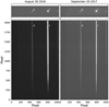 |
Fig. 1. GTC/OSIRIS image through the slit (top panels) and raw science image (bottom panels) for the nights of August 30, 2016 (left panels), and September 25, 2017 (right panels). In this image, the target star is labeled T and the selected reference star is labeled R. |
GTC instrumental configuration used in both observing nights.
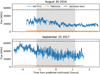 |
Fig. 2. HAT-P-11 and reference star count level of the pixel with the maximum flux inside the extraction aperture for the nights of August 30, 2016 (top panel), and September 25, 2017 (bottom panel). The shaded area marks the duration of the transit and the dashed line marks the saturation levels of the detector. The different saturation levels in the two nights are due to different readout modes adopted. |
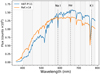 |
Fig. 3. Extracted R1000B grism spectrum of HAT-P-11 (blue) and its reference star (orange). The spectra are not corrected for instrumental response or flux calibrated. The flux of the reference star was multiplied by a factor of 14 to match the flux level of the target for easy viewing. The shaded gray areas indicate the custom passbands used to create the spectroscopic light curves. |
3. Data analysis
The data for both nights were fitted following the procedure of Chen et al. (2018). The analytic transit curve was created using the models of Mandel & Agol (2002) through the batman implementation of Kreidberg (2015). For the limb darkening coefficients (LDC) we adopted a quadratic limb darkening law; the coefficient values u1 and u2 were computed interpolating ATLAS (Kurucz (1979) synthetic stellar spectrum with the code of Espinoza & Jordán (2015). The coefficients were estimated using the stellar parameters of HAT-P-11 presented in Bakos et al. (2010; Teff = 4750 K, [Fe/H] = 0.3 dex, and logg⋆ (cgs) = 4.5). To model the white light curve transit we set as free parameters: the planet-to-star radius ratio Rp ∕Rs, the quadratic limb darkening coefficients u1 and u2, the central time of transit Tmid (for N1 and N2), the orbital semi-major axis over stellar radius a∕Rs, and the orbital inclination i. For the spectroscopic light curves the orbital parameters i and a∕Rs were fixed to the values found for the white light curve. The orbital eccentricity e, period, and argument of the periastron ω were fixed to the values presented in Huber et al. (2017) for all the curves analyzed here.
We created a common-mode noise model by dividing the white light curve by the best fitting transit model, and then each spectroscopic light curve was divided by this common-mode noise. To model the systematic effects present in the data, we used the Gaussian Processes (GP) python implementation provided by george (Ambikasaran et al. 2015). The use of GP to model the red noise has become a standard procedure in light curve analysis (e.g., Gibson et al. 2012). For all the red noise sources, we selected a squared exponential kernel described by
![Mathematical equation: \begin{equation*} k(x_i,x_j) = A^2 \exp \left[ -\sum^{N}_{\alpha=1} \left( \frac{x_{\alpha,i}-x_{\alpha,j}}{L_{\alpha}} \right)^2 \right],\end{equation*}](/articles/aa/full_html/2019/02/aa34063-18/aa34063-18-eq6.png) (1)
(1)
where xi,j are the input vectors associated with the origin of the red noise, in this case a time component and seeing variation measured by the full width at half maximum (FWHM) of the spectral profile in the spatial direction of the target.
Near the position of the target there is a faint star whose flux is inside the spectral extraction aperture for both nights. The GTC telescope was able to observe a transit of HAT-P-11b in August 12, 2017, but unfortunately the target was saturated and in nonlinearity range in most of the in-transit images. We therefore decided to not use this data set in the transmission spectroscopy analysis. The seeing on that night was stable enough to allow us to separate the flux of HAT-P-11 and the contaminant star (see Fig. 4). The flux of the contaminating star was extracted from the nonsaturated pre-transit frames of the data set from August 12, 2017 (see Appendix). We included the flux contamination level by this contaminant in the MCMC procedure to compute an accurate planet-to-star radius ratio (Rp ∕Rs) across the probed wavelength range.
A likelihood function was evaluated iteratively using the python Markov chain Monte Carlo (MCMC) suite emcee (Foreman-Mackey et al. 2013). For the white light curve we used normal priors for the following parameters: the LDC with values centered around the predicted coefficients and with a normal distribution width of 0.1 plus the LDC constrains by Kipping (2013), the orbital inclination and semi-major axis over stellar radius (mean centered around Huber et al. 2017 values), and the flux contamination fraction of the contaminant star. For the spectroscopic light curves we used normal priors for the LDC and the flux contamination fraction of the contaminant star. For the rest of the parameters we used uniform priors for both white light and spectroscopic curves.
The MCMC for the white light curve consisted of 90 independent chains (or walkers) and run for 3000 iterations. For the spectroscopic curves we used 32 independent chains and 3000 iterations. After discarding the first 500 iterations as burn-in period, we computed the median and 1σ values of the posterior distribution for each parameter.
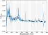 |
Fig. 4. Flux ratio between HAT-P-11 and the contaminant star (blue line). The black dots show the mean flux contamination level inside the 12 bins used to compute HAT-P-11b transmission spectrum. The flux contamination level is relatively stable across the probed wavelength range. |
4. Results and discussion
4.1. White light curve
The white light curves for N1 and N2 are shown in Figs. 5 and 6. Since the reference star is ~ 2.7 magnitudes fainter than HAT-P-11 in V band, the reference star was more affected by seeing variations during the observations and it is the major source of point-to-point variation in the light curve. The seeing variations affect the number of pixels where the point spread function (PSF) is contained and this effect is correlated with the FWHM of the stellar flux. Our light-curve modeling is able to reproduce this noise source and we can recover the transit for each night. Once we subtract the transit model from the light curves, we reach a root mean square (RMS) of the residuals of 519 ppm and 600 ppm for N1 and N2, respectively. The transit parameters and 1σ uncertainties fitted using a joint analysis of N1 and N2 are listed in Table 3.
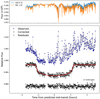 |
Fig. 5. GTC/OSIRIS HAT-P-11b white light transit curve for the night of August 30, 2016. Top panel: measured flux vs. time of HAT-P-11 and the reference star; the flux of the reference was multiplied by a factor of 14 for visualization purposes. Bottom panel: blue points represent the observed time series, the gray dashed line shows the best-fit model (transit model plus systematics and red noise) determined using our MCMC analysis, the black open circles show the light curve after removing the systematic effects and red noise component, while the red line is the best-fitting transit model. All the curves are shown with an arbitrary offset in y-axis. |
MCMC joint analysis results of the white light transit curve of HAT-P-11b.
4.2. Transmission spectrum
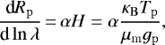
The GTC/OSIRIS transmission spectrum for the joint fit of N1 and N2 is shown in Fig. 7. Table 4 presents the measured planet-to-star radius ratio and 1σ uncertainties for each bin. The spectroscopic light curves and best fit model of each night are shown in the Appendix (Figs. A.3 and A.4). Our joint fit results are consistent with a pure Rayleigh scattering feature when comparedto a flat model (straight line) and Exo-Transmit (Kempton et al. 2017) models with clear (i.e., no clouds) and cloudy atmospheres. The cross-section of the particles that produce the Rayleigh scattering follow a power law 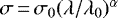 , where λ0 is the cross-section size at the reference wavelength λ0 and α = − 4 (Lecavelier Des Etangs et al. 2008). The change of measured planet-to-star-radius ratio across wavelength is related to the planetary atmospheric scale height and α by
 (2)
(2)
where H is the atmospheric scale height, κB the Boltzmann constant, Tp the temperature of the atmosphere of the planet, μm the mean molecular weight of the planetary atmosphere, and gp is the surface gravity of the planet.
Assuming a hydrogen-dominated atmosphere (μm = 2.37), a planetary temperature of Tp = 878 ± 15 K (Bakos et al. 2010), and adopting gp = 14.08 ± 1.17 m s−2 (computed using the planetary mass of Southworth 2011 and radius of Deming et al. 2011), we find αjoint = −9.86 ± 6.19 for the measured dRp∕d ln λ using the joint fit of N1 and N2. It is worth mentioning that the relatively large uncertainty in αjoint comes from the stellar radius of HAT-P-11 (Eq. (2) needs the planetary radius, not the planet-to-star-radius ratio). Considering the uncertainties, the α value for the joint fit is consistent with Rayleigh scattering from a hydrogen-dominated atmosphere, although the measured value departs from the expected α = −4. This led us to examine in closer detail each observing night.
We re-analyzed the transits for N1 and N2, this time leaving the planet-to-star-radius ratio as free parameter for each night independently (see Table 4 for the measured planet-to-star radius ratio and 1σ uncertainties). Figure 8 presents a comparison of the transmission spectrum of HAT-P-11b for each night fitted independently along with the results of the joint fit. The data from N1 presents a greater Rp ∕Rs versus ln λ slope; if we use the same μm, Tp, and gp values as before we get αN1 = −21.85 ± 9.25. In contrast, the transmission spectrum for N2 is relatively flat and featureless with a slope slightly increasing towards redder wavelengths. One possible explanation for the discrepancy between data sets is stellar activity.
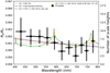 |
Fig. 7. Optical transmission spectrum of HAT-P-11b taken with GTC/OSIRIS for the joint fit of N1 and N2. |
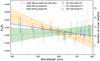 |
Fig. 8. Optical transmission spectrum of HAT-P-11b taken with GTC/OSIRIS for the joint fit (blue), and individual fit for N1 (orange) and N2 (green). The lines and shaded areas represent the best fit and 1σ uncertainty range for N1 (orange) and N2 (green). The data points are shifted in x-axis arbitrarily. |
4.3. The impact of stellar spots
The host star of HAT-P-11b is known to be active, in the discovery paper Bakos et al. (2010) measured a mean Ca II H & K emission activity index of ⟨S⟩ = 0.61. Morris et al. (2017a) studied the evolution of the S-index of HAT-P-11 from 2008 to 2017 using Keck/HIRES data, they found evidence of an activity cycle of close to 10 yr in duration and measured a mean S-index of ⟨S⟩ = 0.58 ± 0.04. The mean S-index measured by Morris et al. (2017a) is equivalent to an activity index of  (see Noyes et al. 1984 for the definition of the
  index), a value representative for stars exhibiting significant stellar activity.
One way in which stellar activity affects the star is the appearance of spots in its surface. There are several transits of HAT-P-11b observed by Kepler where the planet crossed regions with spots (see e.g., Southworth 2011, Fig. 23). Sanchis-Ojeda & Winn (2011) used Kepler data to constrain the orbital obliquity and identified two regions with spots which were interpreted as active regions of the star. Also, using Kepler data, Béky et al. (2014) found evidence of a long-lived spot region in HAT-P-11 that was eclipsed by the planet six times and discovered that the orbital period of HAT-P-11b and the rotational period of the host star are in a period ratio of 6:1. Morris et al. (2017b) studied the spot area coverage and spot distribution across the stellar surface, deducing that  % of the surface is covered by spots and that they are distributed around 16° ± 1° latitude.
Occulted and unocculted stellar spots can affect the flux measurement during a transit, leading to an incorrect estimate of the transit depth (Pont et al. 2013). According to Fraine et al. (2014) the median amplitude of spot crossing events in Kepler band is close to 500 ppm, by visual inspection we did not detect any spot crossing event in either of our data sets which both have rms of the residuals of the order of 500 ppm in the white light curve. The major problem preventing us from detecting occulted spots is the faintness of the reference star, which introduced strong systematics correlated with seeing. Even if there were spot-crossing events in our data sets, their effect on the measured transmission spectrum would be negligible due to the modeling of common-mode noise (CMN) together with Gaussian processes (CMN removes any abrupt change common in wavelength, Gaussian processes treat the spot as time-correlated noise). However, there is still a chance that unocculted spots can be responsible of producing a signal similar to Rayleigh scattering in the transmitted spectrum of the planet for N1.
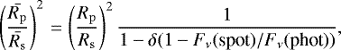
Since spots are regions with different temperature from the average surface temperature, they can introduce a slightly different stellar flux level in some wavelengths creating an effect similar to Rayleigh scattering. To model the effect of unocculted spots during the HAT-P-11 b transit of N1 we followed the approach of prior works (e.g., Sing et al. 2011; McCullough et al. 2014; Chen et al. 2017b; Rackham et al. 2018) in which the observed planet-to-star-radius ratio (without including the effect of limb darkening) can be modeled by
 (3)
(3)
where  is the observed planet-to-star-radius ratio, Rp∕Rs is the true planet-to-star radius-ratio (i.e., not affected by spots), δ is the variable that takes into account the stellar surface area covered by spots or filling factor, Fν (spot) is the flux from the stellar spots, and Fν(phot) is the flux from the stellar photosphere.
To model the flux from the star (and spotted regions) we used PHOENIX stellar models (Husser et al. 2013) for HAT-P-11 (the model with stellar parameters of Teff = 4780 K, log g⋆ (cgs) = 4.5, [Fe/H] = 0.5 dex) and compared it with a grid of spectra with temperatures ranging from 2700 to 7000 K.
We performed a MCMC fitting procedure using Eq. (3) applied to the transmission spectrum of N1 and N2, after removing the last data point (bin centered at 777.5 nm) which presents a different Rp ∕Rs from the rest of the bins probably due to noise added by the nearby telluric O2 line (λ = 760.5 nm, see Fig. 3). We want to emphasize that the main source of noise in this bin is the contaminant star whose wavelength is shifted due to misalignment in the slit (see Fig. 4). If there were no such contaminant star, the majority of the telluric O2 band would have been excluded from our flux integration (see Fig. 3), and the remaining effects should have been corrected by the reference star.
The MCMC was launched with emcee using 80 independent chains and two separate runs: a burn-in run with 10 000 iterations and a main run with 25 000 iterations. Using the posterior distributions to get the median values and 1σ uncertainty range, we get for N1:  and
and  K (see Fig. A.5 for the correlation plot). Morris et al. (2017b) reported a filling factor of
  % for HAT-P-11, a value that the authors suggest as a lower limit due to the assumption made that the stellar spot coverage probed by the transit is representative of the spot coverage of the whole star and the sensitivity of their measurements. In the same article, they claim that HAT-P-11’s filling factor is close to the values of the active K star OU Gem presented in O’Neal et al. (2001) with numbers ranging from δ ≤ 0.04 up to 0.35. Our median value for the filling factor is higher than the values for OU GEM, however the lower limit of the filling factor presented here (δN1 low = 0.45) is close to the numbers presented in O’Neal et al. (2001) and typical values seen in active mid-K dwarfs (e.g., Berdyugina 2005; Andersen & Korhonen 2015) and M dwarfs (e.g., Jackson et al. 2009, Jackson & Jeffries 2012). The difference in temperature between the star and the spot is
  K (considering a stellar model with a temperature of Tphot = 4780 K), which is almost half the temperature presented in Fraine et al. (2014) who measured a ΔT ≈ 900 K based on the largest star spot crossing event observed by their Kepler and Spitzer runs. The surface-to-spot temperature difference of the largest spot crossing event observed by Fraine et al. (2014) is consistent with values found in active K dwarfs, which usually are in the range of 1000–1500 K (e.g., O’Neal et al. 2004; Berdyugina 2005).
The relatively large value and uncertainties found in δ are probably caused by two factors: (1) the uncertainties of the measured planet-to-star-radius ratio allowed several combinations of filling factors and spot temperatures to reproduce the observed transmission spectrum, and (2) the filling factor and the temperature of the stellar spot (which gives Fν(spot)) are correlated, thus producing a very wide posterior probability distribution for the δ parameter.
The second data set could also be affected by bright and dark unocculted spots whose effects cancel out producing the measured flat transmission spectrum (see Fig. 8). It is possible to extend Eq. (3) to include the effects of bright and dark unocculted spots (see Rackham et al. 2018), however due to our uncertainties and the strong correlation between the filling factor and temperature of the spot we decided to use the same MCMC procedure applied for N1 for simplicity. For the flat transmission spectrum of N2 we get  and
and  K (see Fig. A.6 for the correlation plot), a lower filling factor compared to N1 and a spot temperature closer to the adopted temperature of the star.
As a final test we used Eq. (3) to compute the filling factor and spot temperature necessary to go from the transmission spectrum with a slope of N1 to the featureless transmission spectrum of N2. Using the same MCMC fitting procedure as before and without any constrains in the temperature of the spot we get  and
and  K. If we put the constraint that the spot temperature must be higher than the average stellar surface temperature (i.e., bright spots only), we get
  and
and  K. Both results are consistent with each other considering the uncertainties, although the second test preferred higher spot temperatures (
 K) compared to the unconstrained temperaturetest (
 K). The low filling factor values obtained in these tests indicate that a relatively small amount of bright spots can suppress the slope found in N1 producing the flat transmission spectrum of N2.
Anotherway to establish if unocculted spots affected the transmission spectrum is to check the measured transit depth around some atomic lines. For example spots can create an excess in the transit depth at the Na I 589.0 and 589.6 nm doublet while the transit depth decreases in Hα (656.3 nm; see Chen et al. 2017a). We fitted (individually for N1 and N2) several light curves with a bin size of 5 nm of width around the Na I doublet, but this time using the mean FWHM of the absorption lines as input for the GP instead of the FWHM of the spectral profile used in the previous presented results. The reason for this change is that using the FWHM of the absorption lines delivers better results when modeling the red noise in curves produced with narrow wavelength bins.
Figure 9 shows the planet-to-star-radius ratio measured around the Na I doublet for N1 (top panel) and N2 (bottom panel), compared to the same Exo-Transmit models presented in Fig. 7 and the expected Rp ∕Rs using the best fitting model of Eq. (3) for N1 and N2. The first dataset (N1) presents an excess in the transit depth for the bin centered at the Na I doublet in agreement with the atmospheric models for HAT-P-11b and the unocculted spot model. In the second data set (N2) the excess in Rp∕Rs at the bin centered at the Na I doublet disappears, and the overall transmission spectrum is more consistent with a flat model, as predicted by the unocculted spot model for N2.
In the case of Hα our measurements are not precise enough to detect the decrease in Rp ∕Rs around this line and differentiate it from a flat model (see Fig. 10).
Based on the transmission spectrum slope, unocculted spot modeling, and the transit depth excess detected in Na I in N1 and not in N2, we are confident that the measured transmission spectrum of N1 was affected by stellar spots mimicking a feature similar to Rayleigh scattering.
Measured Rp∕Rs for HAT-P-11b.
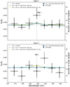 |
Fig. 9. Transmission spectrum of HAT-P-11b around the Na I 589.0 and 589.6 nm doublet for the individual fit of N1 (top panel) and N2 (bottom panel). |
5. Conclusions
We present here an analysis of two primary transits of the Neptune-sized exoplanet HAT-P-11b taken with GTC/OSIRIS instrument. We were able to obtain long-slit spectra of HAT-P-11 and one reference star for the nights of August 30, 2016, and September 25, 2017. Integrating the flux of both stars in different passbands, we created several light curves to measure the change in transit depth across the wavelength range of λ 400–785 nm.The light curves for both nights were fitted jointly and individually using a Bayesian MCMC procedure that takes into accountthe systematic effects present in the data.
The GTC/OSIRIS transmission spectrum of HAT-P-11b obtained with a joint MCMC fit presents a slope towards blue wavelengths. The joint fit results are consistent with a pure Rayleigh scattering feature when compared to a flat model (straight line) and synthetic atmosphere models with clear and cloudy atmospheres. Assuming that this slope was caused by small particles present in the atmosphere of the planet and adopting a planetary equilibrium temperature of Tp = 878 ± 15 K and a molecular weight of μm = 2.37, we measured αjoint = −9.86 ± 6.19. Considering uncertainties, this αjoint value is in the expected Rayleigh scattering range caused by hydrogen-dominated atmospheres (α = −4), although strong assumptions were made when computing this parameter (temperature of the planet and molecular weight). A closer inspection to each individual night revealed that the transmission spectrum for HAT-P-11b taken on August 30, 2016, has a significant slope when compared to the transmission spectrum on the night of September 25, 2017, which is mostly featureless and flat.
The difference in the observed transmission spectrum between the two data sets could be attributed to stellar activity; more specifically, to a greater number of unocculted stellar spots during N1. When modeling the amount of stellar surface area covered by dark spots and their temperature to reproduce the results of the August 2016 data set, we find  ,
,  K and
K and  K. Although our uncertainties in the filling factor are relatively large, the lower limit is in agreement with values seen in active mid-K dwarfs and M stars. The origin of the large uncertainties in the filling factor comes from the fact that δ and Tspot are strongly correlated.
Additionally, we modeled the filling factor and spot temperature needed to suppress the slope of the first data set to obtain the flat transmission spectrum of the second night for two cases: (1) setting the spot temperature completely free, and (2) forcing the spot temperature to be greater than the average stellar surface temperature (i.e., bright spots). For the first case we get  and
and  K and for the second
  and
and  K. Based on these results a relative small amount of bright spots present in the star in the second night could produce the observed flat transmission spectrum, assuming that the spectrum of N1 is a closer representation to the true spectrum of the planet.
Since stellar spots can also affect the intensity of some spectral lines we also compared the transit depth around the Na I doublet (λ 589.0 and 589.6 nm) for both nights, finding that the transit in the first data set is deeper around the Na I doublet than the nearby continuum while for the second night the transmission spectrum is flat; this is consistent with a major presence of unocculted dark spots during the transit of N1 compared to N2. The same analysis was performed for Hα (λ 656.3 nm), however our transit depth measurements around this line are not precise enough to detect a change between N1 and N2.
Based on the fact that the slope in the transmission spectrum is found in N1 but not N2 and the comparison between the transit depth around Na I lines for N1 and N2, we conclude that the transmission spectrum for N1 was affected by stellar activity in the form of unocculted dark spots. The second data set could also be affected by bright and dark unocculted spots whose effects cancel out producing the measured flat transmission spectrum for N2, or simply due to a low stellar activity epoch.
In light of our results for HAT-P-11b, we advocate repeated observations of exoplanet transmission spectroscopy studies to account for possible stellar variability. Simultaneous/contemporary activity monitoring is crucial to establish the true nature of Rayleigh scattering features detected in exoplanets orbiting active stars.
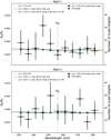 |
Fig. 10. Transmission spectrum of HAT-P-11b around Hα (656.3) nm for the individual fit of N1 (top panel) and N2 (bottom panel). |
Acknowledgements
Based on observations made with the Gran Telescopio Canarias (GTC), installed in the Spanish Observatorio del Roque de los Muchachos of the Instituto de Astrofísica de Canarias, in the island of La Palma. G.C. also acknowledges the support by the National Natural Science Foundation of China (Grant No. 11503088) and the Natural Science Foundation of Jiangsu Province (Grant No. BK20151051). Software: ipython (Pérez & Granger 2007), numpy (van der Walt et al. 2011), scipy (Jones et al. 2001), matplotlib (Hunter 2007), PyDE (https://github.com/hpparvi/PyDE). This research made use of Astropy, a community-developed core Python package for Astronomy (Astropy Collaboration 2013, 2018). Correlation plot for N1 and N2 spot modeling done with Corner (Foreman-Mackey 2016).
Appendix A: Additional figures
A.1. Saturated images for August 12, 2017
The night of August 12, 2017, GTC observed a transit of HAT-P-11b; however, the target was saturated in a large fraction of images and we decided to not use this data set to obtain the transmission spectrum of this planet. During this night, the seeing conditions were good enough to separate the flux of HAT-P-11 and a nearby star, hence we used this data set to establish the flux contamination of including this nearby star inside the extraction aperture. Figure A.1 shows the flux level of the pixel with the maximum flux inside the extraction aperture during the night (top panel) and the saturated pixels along wavelength of the time series (bottom panel). The flux of the contaminant star was extracted using the pre-transit nonsaturated images.
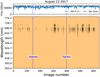 |
Fig. A.1. HAT-P-11 count level of the pixel with the maximum flux inside the extraction aperture (top panel) and saturated pixels of the time series (bottom panel) for the night of August 12, 2017. In the bottom panel the saturated pixels are shown in black while the orange pixels are below the saturation level. The flux of the contaminant star was extracted using the pre-transit nonsaturated images. |
A.2. Light-curve fitting tests
We compared the transmission spectrum of HAT-P-11b obtained by fitting the spectroscopic light curves with and without Gaussianprocesses (GPs) for each individual nights. We tested several models with different baseline functions and parameters. For the final comparison we selected the models with the lowest Bayesian Information Criterion (BIC) value. The two non-GP baseline models selected were
 (A.1)
(A.1)
and
 (A.2)
(A.2)
where ci are fitted coefficients, t is the time, Sy is the FWHM in spatial direction, and Py is the pixel position of the center of the PSF of the spectral profile. To account for the effect of red noise in the data, we used the time-averaging method (Pont et al. 2006).
Figure A.2 presents the transmission spectrum obtained with and without GPs for the baseline models p1 and p2. Both methods show consistent results and the slope in the transmission spectrum does not change significantly.
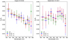 |
Fig. A.2. Comparison between fitting procedures for the individual data sets taken on August 30, 2016 (left panel), and September 25, 2017 (right panel). The green points are the results obtained with GPs and the blue squares and red triangles show the results obtained without GPs and different baseline functions. |
A.3. Spectroscopic light curves
In this section of the appendix we present the spectroscopic light curves of HAT-P-11b for the nights of August 30, 2016, and September 25, 2017.
A.4. Correlation plots
Here we present the correlation plots of the MCMC fitting procedure of Eq. (3) for N1 and N2.
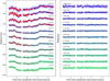 |
Fig. A.3. Spectroscopic light curves obtained using the custom passbands (see Fig. 3) for HAT-P-11b transit of August 30, 2016. Left panel: light curves after removing the common-mode systematics and best fit model (red line). Right panel: residuals of the light curves after removing a transit model and systematic effects. |
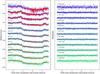 |
Fig. A.4. Spectroscopic light curves obtained using the custom passbands (see Fig. 3) for HAT-P-11b transit of September 25, 2017. Left panel: light curves after removing the common-mode systematics and best fit model (red line). Right panel: residuals of the light curves after removing a transit model and systematic effects. |
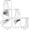 |
Fig. A.5. Correlation plot for the spot coverage model for N1. |
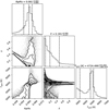 |
Fig. A.6. Correlation plot for the spot coverage model for N2. |
References
- Allart, R., Bourrier, V., Lovis, C., et al. 2018, Science, 362, 1384 [NASA ADS] [CrossRef] [Google Scholar]
- Ambikasaran, S., Foreman-Mackey, D., Greengard, L., Hogg, D. W., & O’Neil, M. 2015, IEEE Trans. Pattern Anal. Mach. Intell., 38, 252 [NASA ADS] [CrossRef] [Google Scholar]
- Andersen, J. M., & Korhonen, H. 2015, MNRAS, 448, 3053 [NASA ADS] [CrossRef] [Google Scholar]
- Astropy Collaboration (Robitaille, T. P., et al.) 2013, A&A, 558, A33 [NASA ADS] [CrossRef] [EDP Sciences] [Google Scholar]
- Astropy Collaboration (Price-Whelan, A. M., et al.) 2018, AJ, 156, 123 [Google Scholar]
- Bakos, G. Á., Torres, G., Pál, A., et al. 2010, ApJ, 710, 1724 [NASA ADS] [CrossRef] [Google Scholar]
- Bean, J. L., Miller-Ricci Kempton, E., & Homeier, D. 2010, Nature, 468, 669 [NASA ADS] [CrossRef] [PubMed] [Google Scholar]
- Béky, B., Holman, M. J., Kipping, D. M., & Noyes, R. W. 2014, ApJ, 788, 1 [NASA ADS] [CrossRef] [Google Scholar]
- Berdyugina, S. V. 2005, Liv. Rev. Sol. Phys., 2, 8 [Google Scholar]
- Cepa, J., Aguiar, M., Escalera, V. G., et al. 2000, SPIE Conf. Ser, 4008, 623 [Google Scholar]
- Charbonneau, D., Brown, T. M., Noyes, R. W., & Gilliland, R. L. 2002, ApJ, 568, 377 [NASA ADS] [CrossRef] [Google Scholar]
- Chen, G., Pallé, E., Nortmann, L., et al. 2017a, A&A, 600, L11 [NASA ADS] [CrossRef] [EDP Sciences] [Google Scholar]
- Chen, G., Guenther, E. W., Pallé, E., et al. 2017b, A&A, 600, A138 [NASA ADS] [CrossRef] [EDP Sciences] [Google Scholar]
- Chen, G., Palle, E., Welbanks, L., et al. 2018, A&A, 616, A145 [NASA ADS] [CrossRef] [EDP Sciences] [Google Scholar]
- Cutri, R. M., Skrutskie, M. F., van Dyk, S., et al. 2003, VizieR Online Data Catalog: II/246 [Google Scholar]
- Deming, D., Sada, P. V., Jackson, B., et al. 2011, ApJ, 740, 33 [NASA ADS] [CrossRef] [Google Scholar]
- Diamond-Lowe, H., Berta-Thompson, Z., Charbonneau, D., & Kempton, E. M.-R. 2018, AJ, 156, 42 [NASA ADS] [CrossRef] [Google Scholar]
- Dragomir, D., Benneke, B., Pearson, K. A., et al. 2015, ApJ, 814, 102 [NASA ADS] [CrossRef] [Google Scholar]
- Eastman, J., Siverd, R., & Gaudi, B. S. 2010, PASP, 122, 935 [NASA ADS] [CrossRef] [Google Scholar]
- Espinoza, N., & Jordán, A. 2015, MNRAS, 450, 1879 [NASA ADS] [CrossRef] [Google Scholar]
- Foreman-Mackey, D. 2016, J. Open Source Softw., 1, 24 [Google Scholar]
- Foreman-Mackey, D., Hogg, D. W., Lang, D., & Goodman, J. 2013, PASP, 125, 306 [CrossRef] [Google Scholar]
- Fraine, J., Deming, D., Benneke, B., et al. 2014, Nature, 513, 526 [NASA ADS] [CrossRef] [Google Scholar]
- Fukui, A., Narita, N., Kurosaki, K., et al. 2013, ApJ, 770, 95 [NASA ADS] [CrossRef] [Google Scholar]
- Gibson, N. P., Aigrain, S., Roberts, S., et al. 2012, MNRAS, 419, 2683 [NASA ADS] [CrossRef] [Google Scholar]
- Henden, A. A., Levine, S., Terrell, D., & Welch, D. L. 2015, AAS Meeting Abstracts, 336.16 [Google Scholar]
- Hirano, T., Narita, N., Shporer, A., et al. 2011, PASJ, 63, 531 [NASA ADS] [Google Scholar]
- Høg, E., Fabricius, C., Makarov, V. V., et al. 2000, A&A, 355, L27 [Google Scholar]
- Horne, K. 1986, PASP, 98, 609 [NASA ADS] [CrossRef] [EDP Sciences] [Google Scholar]
- Huber, K. F., Czesla, S., & Schmitt, J. H. M. M. 2017, A&A, 597, A113 [NASA ADS] [CrossRef] [EDP Sciences] [Google Scholar]
- Hunter, J. D. 2007, Comput. Sci. Eng., 9, 90 [NASA ADS] [CrossRef] [Google Scholar]
- Husser, T.-O., Wende-von Berg, S., Dreizler, S., et al. 2013, A&A, 553, A6 [NASA ADS] [CrossRef] [EDP Sciences] [Google Scholar]
- Jackson, R. J., & Jeffries, R. D. 2012, MNRAS, 423, 2966 [NASA ADS] [CrossRef] [Google Scholar]
- Jackson, R. J., Jeffries, R. D., & Maxted, P. F. L. 2009, MNRAS, 399, L89 [NASA ADS] [CrossRef] [Google Scholar]
- Jones, E., Oliphant, T., Peterson, P., et al. 2001, SciPy: Open Source Scientific Tools for Python [Google Scholar]
- Kempton, E. M.-R., Lupu, R., Owusu-Asare, A., Slough, P., & Cale, B. 2017, PASP, 129, 044402 [NASA ADS] [CrossRef] [Google Scholar]
- Kipping, D. M. 2013, MNRAS, 435, 2152 [Google Scholar]
- Kirk, J., Wheatley, P. J., Louden, T., et al. 2017, MNRAS, 468, 3907 [NASA ADS] [CrossRef] [Google Scholar]
- Knutson, H. A., Dragomir, D., Kreidberg, L., et al. 2014, ApJ, 794, 155 [NASA ADS] [CrossRef] [Google Scholar]
- Kreidberg, L. 2015, PASP, 127, 1161 [NASA ADS] [CrossRef] [Google Scholar]
- Kreidberg, L., Bean, J. L., Désert, J.-M., et al. 2014a, ApJ, 793, L27 [NASA ADS] [CrossRef] [Google Scholar]
- Kreidberg, L., Bean, J. L., Désert, J.-M., et al. 2014b, Nature, 505, 69 [NASA ADS] [CrossRef] [Google Scholar]
- Kurucz, R. L. 1979, ApJS, 40, 1 [NASA ADS] [CrossRef] [Google Scholar]
- Lecavelier Des Etangs, A., Vidal-Madjar, A., Désert, J. M., & Sing, D. 2008, A&A, 485, 865 [NASA ADS] [CrossRef] [EDP Sciences] [Google Scholar]
- Lecavelier Des Etangs, A., Sirothia, S. K., Gopal-Krishna, & Zarka, P. 2013, A&A, 552, A65 [NASA ADS] [CrossRef] [EDP Sciences] [Google Scholar]
- Mandel, K., & Agol, E. 2002, ApJ, 580, L171 [NASA ADS] [CrossRef] [Google Scholar]
- Mansfield, M., Bean, J. L., Oklopčić, A., et al. 2018, ApJ, 868, L34 [NASA ADS] [CrossRef] [Google Scholar]
- McCullough, P. R., Crouzet, N., Deming, D., & Madhusudhan, N. 2014, ApJ, 791, 55 [NASA ADS] [CrossRef] [Google Scholar]
- Morris, B. M., Hawley, S. L., Hebb, L., et al. 2017a, ApJ, 848, 58 [NASA ADS] [CrossRef] [Google Scholar]
- Morris, B. M., Hebb, L., Davenport, J. R. A., Rohn, G., & Hawley, S. L. 2017b, ApJ, 846, 99 [NASA ADS] [CrossRef] [Google Scholar]
- Nascimbeni, V., Piotto, G., Pagano, I., et al. 2013, A&A, 559, A32 [NASA ADS] [CrossRef] [EDP Sciences] [Google Scholar]
- Nikolov, N., Sing, D. K., Burrows, A. S., et al. 2015, MNRAS, 447, 463 [NASA ADS] [CrossRef] [Google Scholar]
- Nikolov, N., Sing, D. K., Fortney, J. J., et al. 2018, Nature, 557, 526 [NASA ADS] [CrossRef] [Google Scholar]
- Noyes, R. W., Hartmann, L. W., Baliunas, S. L., Duncan, D. K., & Vaughan, A. H. 1984, ApJ, 279, 763 [NASA ADS] [CrossRef] [Google Scholar]
- O’Neal, D., Neff, J. E., Saar, S. H., & Mines, J. K. 2001, AJ, 122, 1954 [NASA ADS] [CrossRef] [Google Scholar]
- O’Neal, D., Neff, J. E., Saar, S. H., & Cuntz, M. 2004, AJ, 128, 1802 [NASA ADS] [CrossRef] [Google Scholar]
- Oshagh, M., Santos, N. C., Ehrenreich, D., et al. 2014, A&A, 568, A99 [NASA ADS] [CrossRef] [EDP Sciences] [Google Scholar]
- Pérez, F., & Granger, B. E. 2007, Comput. Sci. Eng., 9, 21 [Google Scholar]
- Pont, F., Zucker, S., & Queloz, D. 2006, MNRAS, 373, 231 [NASA ADS] [CrossRef] [Google Scholar]
- Pont, F., Sing,D. K., Gibson, N. P., et al. 2013, MNRAS, 432, 2917 [NASA ADS] [CrossRef] [Google Scholar]
- Quirrenbach, A., Amado, P. J., Caballero, J. A., et al. 2014, in Ground-based and Airborne Instrumentation for Astronomy V, SPIE Conf. Ser., 9147, 91471F [Google Scholar]
- Rackham, B. V., Apai, D., & Giampapa, M. S. 2018, ApJ, 853, 122 [NASA ADS] [CrossRef] [Google Scholar]
- Redfield, S., Endl, M., Cochran, W. D., & Koesterke, L. 2008, ApJ, 673, L87 [NASA ADS] [CrossRef] [MathSciNet] [Google Scholar]
- Sanchis-Ojeda, R., & Winn, J. N. 2011, ApJ, 743, 61 [NASA ADS] [CrossRef] [Google Scholar]
- Sing, D. K., Pont, F., Aigrain, S., et al. 2011, MNRAS, 416, 1443 [NASA ADS] [CrossRef] [Google Scholar]
- Sing, D. K., Lecavelier des Etangs, A., Fortney, J. J., et al. 2013, MNRAS, 436, 2956 [NASA ADS] [CrossRef] [Google Scholar]
- Sing, D. K., Wakeford, H. R., Showman, A. P., et al. 2015, MNRAS, 446, 2428 [NASA ADS] [CrossRef] [Google Scholar]
- Snellen, I. A. G., Albrecht, S., de Mooij, E. J. W., & Le Poole, R. S. 2008, A&A, 487, 357 [NASA ADS] [CrossRef] [EDP Sciences] [Google Scholar]
- Southworth, J. 2011, MNRAS, 417, 2166 [NASA ADS] [CrossRef] [Google Scholar]
- Stevenson, K. B., Harrington, J., Nymeyer, S., et al. 2010, Nature, 464, 1161 [NASA ADS] [CrossRef] [PubMed] [Google Scholar]
- Tsiaras, A., Rocchetto, M., Waldmann, I. P., et al. 2016, ApJ, 820, 99 [NASA ADS] [CrossRef] [Google Scholar]
- Tsiaras, A., Waldmann, I. P., Zingales, T., et al. 2018, AJ, 155, 156 [NASA ADS] [CrossRef] [Google Scholar]
- van der Walt, S., Colbert, S. C., & Varoquaux, G. 2011, Comput. Sci. Eng., 13, 22 [Google Scholar]
- Wakeford, H. R., Sing, D. K., Deming, D., et al. 2018, AJ, 155, 29 [Google Scholar]
- Winn, J. N., Johnson, J. A., Howard, A. W., et al. 2010, ApJ, 723, L223 [NASA ADS] [CrossRef] [Google Scholar]
- Yee, S. W., Petigura, E. A., Fulton, B. J., et al. 2018, AJ, 155, 255 [NASA ADS] [CrossRef] [Google Scholar]
Saturation levels taken from http://www.gtc.iac.es/instruments/osiris/media/OSIRIS-USER-MANUAL_v3_1.pdf
All Tables
All Figures
|
Fig. 1. GTC/OSIRIS image through the slit (top panels) and raw science image (bottom panels) for the nights of August 30, 2016 (left panels), and September 25, 2017 (right panels). In this image, the target star is labeled T and the selected reference star is labeled R. |
| In the text | |
|
Fig. 2. HAT-P-11 and reference star count level of the pixel with the maximum flux inside the extraction aperture for the nights of August 30, 2016 (top panel), and September 25, 2017 (bottom panel). The shaded area marks the duration of the transit and the dashed line marks the saturation levels of the detector. The different saturation levels in the two nights are due to different readout modes adopted. |
| In the text | |
|
Fig. 3. Extracted R1000B grism spectrum of HAT-P-11 (blue) and its reference star (orange). The spectra are not corrected for instrumental response or flux calibrated. The flux of the reference star was multiplied by a factor of 14 to match the flux level of the target for easy viewing. The shaded gray areas indicate the custom passbands used to create the spectroscopic light curves. |
| In the text | |
|
Fig. 4. Flux ratio between HAT-P-11 and the contaminant star (blue line). The black dots show the mean flux contamination level inside the 12 bins used to compute HAT-P-11b transmission spectrum. The flux contamination level is relatively stable across the probed wavelength range. |
| In the text | |
|
Fig. 5. GTC/OSIRIS HAT-P-11b white light transit curve for the night of August 30, 2016. Top panel: measured flux vs. time of HAT-P-11 and the reference star; the flux of the reference was multiplied by a factor of 14 for visualization purposes. Bottom panel: blue points represent the observed time series, the gray dashed line shows the best-fit model (transit model plus systematics and red noise) determined using our MCMC analysis, the black open circles show the light curve after removing the systematic effects and red noise component, while the red line is the best-fitting transit model. All the curves are shown with an arbitrary offset in y-axis. |
| In the text | |
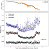 |
Fig. 6. As in Fig. 5 but for the night of September 25, 2017. |
| In the text | |
|
Fig. 7. Optical transmission spectrum of HAT-P-11b taken with GTC/OSIRIS for the joint fit of N1 and N2. |
| In the text | |
|
Fig. 8. Optical transmission spectrum of HAT-P-11b taken with GTC/OSIRIS for the joint fit (blue), and individual fit for N1 (orange) and N2 (green). The lines and shaded areas represent the best fit and 1σ uncertainty range for N1 (orange) and N2 (green). The data points are shifted in x-axis arbitrarily. |
| In the text | |
|
Fig. 9. Transmission spectrum of HAT-P-11b around the Na I 589.0 and 589.6 nm doublet for the individual fit of N1 (top panel) and N2 (bottom panel). |
| In the text | |
|
Fig. 10. Transmission spectrum of HAT-P-11b around Hα (656.3) nm for the individual fit of N1 (top panel) and N2 (bottom panel). |
| In the text | |
|
Fig. A.1. HAT-P-11 count level of the pixel with the maximum flux inside the extraction aperture (top panel) and saturated pixels of the time series (bottom panel) for the night of August 12, 2017. In the bottom panel the saturated pixels are shown in black while the orange pixels are below the saturation level. The flux of the contaminant star was extracted using the pre-transit nonsaturated images. |
| In the text | |
|
Fig. A.2. Comparison between fitting procedures for the individual data sets taken on August 30, 2016 (left panel), and September 25, 2017 (right panel). The green points are the results obtained with GPs and the blue squares and red triangles show the results obtained without GPs and different baseline functions. |
| In the text | |
|
Fig. A.3. Spectroscopic light curves obtained using the custom passbands (see Fig. 3) for HAT-P-11b transit of August 30, 2016. Left panel: light curves after removing the common-mode systematics and best fit model (red line). Right panel: residuals of the light curves after removing a transit model and systematic effects. |
| In the text | |
|
Fig. A.4. Spectroscopic light curves obtained using the custom passbands (see Fig. 3) for HAT-P-11b transit of September 25, 2017. Left panel: light curves after removing the common-mode systematics and best fit model (red line). Right panel: residuals of the light curves after removing a transit model and systematic effects. |
| In the text | |
|
Fig. A.5. Correlation plot for the spot coverage model for N1. |
| In the text | |
|
Fig. A.6. Correlation plot for the spot coverage model for N2. |
| In the text | |
Current usage metrics show cumulative count of Article Views (full-text article views including HTML views, PDF and ePub downloads, according to the available data) and Abstracts Views on Vision4Press platform.
Data correspond to usage on the plateform after 2015. The current usage metrics is available 48-96 hours after online publication and is updated daily on week days.
Initial download of the metrics may take a while.