| Issue |
A&A
Volume 622, February 2019
|
|
|---|---|---|
| Article Number | A58 | |
| Number of page(s) | 24 | |
| Section | Extragalactic astronomy | |
| DOI | https://doi.org/10.1051/0004-6361/201833834 | |
| Published online | 28 January 2019 | |
Nonaxisymmetric models of galaxy velocity maps
1
Museo Storico della Fisica e Centro Studi e Ricerche Enrico Fermi, 00184 Rome, Italy
e-mail: This email address is being protected from spambots. You need JavaScript enabled to view it.
2
Istituto dei Sistemi Complessi, Consiglio Nazionale delle Ricerche, 00185 Roma, Italy
3
Istituto Nazionale Fisica Nucleare, Dipartimento di Fisica, Università “Sapienza”, 00185 Roma, Italy
4
University of Oulu, Astronomy Research Unit, PO Box 3000 90014, Finland
5
Instituto de Astrofísica de Canarias, 38205 La Laguna, Tenerife, Spain
6
Departamento de Astrofísica, Universidad de La Laguna, 38206 La Laguna, Tenerife, Spain
Received:
12
July
2018
Accepted:
27
November
2018
Abstract
Galaxy velocity mapsoften show the typical pattern of a rotating disk, consistent with the dynamical model where emitters rotate in circular orbits around the galactic center. The simplest template used to fit these maps consists in the rotating disk model (RDM) where the amplitude of circular velocities is fixed by the observed velocity profile along the kinematic axis. A more sophisticated template is the rotating tilted-ring model (RTRM) that takes into account the presence of warps and allows a radius-dependent orientation of the kinematic axis. In both cases, axisymmetry is assumed and residuals between the observed and the model velocity fields are interpreted as noncircular motions. We show that if a galaxy is not axisymmetric, there is an intrinsic degeneracy between a rotational and a radial velocity field. We then introduce a new galaxy template, the radial ellipse model (REM), that is not axisymmetric and has a purely radial velocity field with an amplitude that is correlated with the major axis of the ellipse. We show that best fits to the observed two-dimensional velocity fields of 28 galaxies extracted from the THINGS sample with both the REM and the RDM give residuals with similar amplitudes, where the REM residuals trace nonradial motions. Best fits obtained with the RTRM, because of its larger number of free parameters, give the smallest residuals: however, we argue that this does not necessarily imply that the RTRM gives the most accurate representation of a galaxy velocity field. Instead, we show that this method is not able to disentangle between circular and radial motions for the case of nonaxisymmetric systems. We then discuss a refinement of the REM, able to describe the properties of a more heterogeneous velocity field where circular and radial motions are respectively predominant at small and large distances from the galaxy center. Finally, we consider the physical motivation of the REM, and discuss how the interpretation of galactic dynamics changes if one assumes that the main component of a galaxy velocity field is modeled as a RDM/RTRM or as a REM.
Key words: galaxies: kinematics and dynamics / galaxies: fundamental parameters / galaxies: structure
© ESO 2019
1. Introduction
Two-dimensional velocity maps of many galaxies show the distinctive pattern of a rotating axisymmetric disk, that is, the typical velocity gradient where on one side of the nucleus spectral lines of stars (or other emitters) are shifted toward the blue region of the spectrum with respect to the systemic velocity and on the opposite side lines are shifted toward the red spectral region (Rubin 1983). These observations are usually interpreted as originating from the Doppler shift caused by the circular motion of the various emitters around the center of the galaxy. The dynamical model that is derived from these data postulates that a galaxy is close to a steady rotating axisymmetric disk configuration in which centripetal and centrifugal forces compensate each other at all radii. By comparing the line-of-sight velocity profile with the amount of luminous matter it is concluded that, in order to maintain such a steady state, a large amount of dark matter is then needed (van der Kruit & Bosma 1978; Thonnard et al. 1978; Bosma 1981). In particular, evidence for the existence of dark matter halos around spiral galaxies comes mainly from the flatness of the rotation curves outside the visible region of galaxies with the extended HI emissions (see Sofue & Rubin 2001, for a review).
Coherently with this model, observed galaxy velocity maps are usually fitted with a template consisting of a rotating disk model (RDM): this assumes that a disk (axisymmetric) galaxy is in circular rotation in a plane about a central axis. The amplitude of the circular velocities as a function of the distance from the center, that is, the rotation curve, is obtained from the observed one-dimensional (1D) line-of-sight (LOS) velocity profile measured along the galaxy kinematic axis1 (Begeman 1989; Schoenmakers et al. 1997; Beckman et al. 2004; Trachternach et al. 2008; Erroz-Ferrer et al. 2012, 2015). The best-fitting RDM is the one that minimizes the residuals between the rotational model velocities, computed for a specific value of the inclination angle2 of the disk i and the actual data. Significant residuals are typically measured in such fitting procedures – of the order of 20–30% of the maximum circular velocity or even larger – and these are attributed to noncircular (e.g., radial, random, etc.) motions (see, e.g., Jorsater & van Moorsel 1995; Zurita et al. 2004; Trachternach et al. 2008; Sellwood & Sánchez 2010; Erroz-Ferrer et al. 2015).
The RDM is only compatible with observations at first order: for instance in the case of an ideal rotating disk, by construction, the kinematic axis must be aligned with the projected semimajor axis, whereas it is frequently observed that galaxies show a significant angular offset between these two axes (see, e.g., Erroz-Ferrer et al. 2015). In addition, it is known that many galaxies exhibit bars and/or warps that can locally distort the velocity field and that cannot be described by the simple axisymmetric disk model. Indeed, several observations have shown that most disks exhibit a wealth of nonaxisymmetric structures (Rix & Zaritsky 1995; Kornreich et al. 2000; Laine et al. 2014) and that the stellar disk in a typical spiral galaxy is significantly lopsided, indicating asymmetry in the disk mass distribution. Lopsidedness is quite typical in disk galaxies (Jog & Combes 2009) and it may be interpreted as a pattern of elliptical orbits (Baldwin et al. 1980; Song 1983).
A simple disk is clearly not a realistic representation of a galaxy, but introducing a more complex shape is very difficult and requires modeling systems of increasing complexity. In this respect a relatively simple way to take into account the fact that a galaxy disk may exhibit warps was to introduce the rotating tilted-ring model (RTRM). In particular, the physical motivation to hypothesize this template was to accommodate warps in HI disks originally detected for the case of M83 (Rogstad et al. 1974). In that case it was indeed observed that the velocity field was incompatible with a simple RDM and it was thus proposed to interpret the observations in terms of a warped disk where all the mass moves in circular rotation around the galaxy center, but where the material that lies beyond the optical image moves in orbits inclined with respect to the central plane. More specifically, the inclination of the orbits was thought to depend on the distance from the galaxy center. In this way the RTRM, similarly to the RDM, assumes axisymmetry but it also postulates that a galaxy can be described as a set of concentric rings where each ring is characterized by a circular velocity and an orientation (see below). Changing the orientation angles as a function of the distance from the galaxy center in a continuous way makes it possible to obtain a better fit than with the RDM. As for the case of the RDM, the RTRM residuals are interpreted as the signature of noncircular motions. A great effort is then devoted to characterizing residuals (i.e., the difference between the actual galaxy velocity field and that of the best-fit RTRM) that are interpreted to trace motions deviating from purely rotational ones (Trachternach et al. 2008; Oh et al. 2008; Erroz-Ferrer et al. 2015).
The existence of warps has been proven independently from kinematic studies, namely by observing both edge-on galaxies (Sancisi 1976; Reshetnikov & Combes 1998; Schwarzkopf & Dettmar 2001; García-Ruiz et al. 2002; Sánchez-Saavedra et al. 2003) and the Milky Way (Levine et al. 2006; Kalberla et al. 2007; Reylé et al. 2009). These observations give a straightforward physical explanation for a twisted position angle that justifies, from the physical point of view, the use of the RTRM. Of course the presence of a warp is compatible with the RTRM but it does not prove either that a galaxy is axisymmetric or that emitters move on stable circular orbits: these are however the two assumptions that are at the basis of the RTRM.
In this paper we study the determination of a galaxy velocity field, and in particular the problem of disentangling radial from circular motions, in the case where the assumption of axisymmetry is not valid to describe the shape of a galaxy. We show that it is possible to build a simple template that is very different from a RDM but that fits the observed galaxy two-dimensional (2D) maps equally well (but both models give worse fits than the RTRM). This template, referred to hear as the radial ellipse model (REM), (i) breaks axisymmetry, i.e., it is an (infinitely thin) ellipse, and (ii) has a purely radial velocity field directed outwards that (iii) has a strong correlation with the direction of the major axis of the system. We use the three models (i.e., the RDM, the RTRM, and the REM) to fit the 2D velocity maps of the galaxy measured by The HI Nearby Galaxy Survey (THINGS; Walter et al. 2008); we then compare the results between the fits and discuss the different interpretation of the galaxy velocity fields and dynamical models in the different cases. In particular, by considering the properties of some toy models with physically motivated and complex velocity fields, we show that the better fit typically provided by the RTRM does not necessarily correspond to the best representation of a given velocity field. Most notably we show that this method, as the RDM, may confuse rotational and radial motions if the system is not axisymmetric.
The paper is organized as follows: in Sect. 2 the properties of some simple toy models allow us to illustrate the problems encountered in disentangling the different motions (i.e., radial and circular) in an ideal galaxy velocity map if the assumption of axisymmetry is not valid. In Sect. 3 we introduce the REM, discussing its properties and the various parameters used in the fitting procedure. We also detail the fitting procedures of the three different models. We then present in Sect. 4 the results of the fits with the RDM, with the REM and with the RTRM of a sub-sample of 28 galaxies extracted from the THINGS sample; we also consider a template that consists in a combination of the RDM and the REM. We then illustrate the physical motivation of the REM and, finally, in Sect. 5, we draw our main conclusions, discussing the consequences of the breaking of axisymmetry on the interpretation of galaxy dynamics and the estimation of the mass of a galaxy.
2. Circular and radial motions in nonaxisymmetric objects
The observed 2D velocity field of a galaxy corresponds to the projection onto the sky of a 3D one, where measurements always give only the radial component of the velocity of an emitter in the direction of the observer, that is, the LOS velocity. By modeling a galaxy as a disk (that is obviously axisymmetric), the projected LOS velocities3 can be written as (see, e.g., Begeman 1987; Beckman et al. 2004)
 (1)
(1)
where, following standard conventions, i is the inclination angle of the observer, i.e., the angle between their LOS and a vector orthogonal to the plane of the galaxy, r and η are polar coordinates (with the angle η defined relative to the axis orthogonal to the observer LOS) in the plane of the sky of a point with coordinates R and θ in the plane of the galaxy, and vθ and vR are the components of the velocity field, tangential and radial, respectively, given in polar coordinates (R, θ) in the plane of the galaxy. The polar coordinates in the two frames of references are related by the transformation
 (2)
(2)
If the system has purely circular velocities and is axisymmetric then vR = 0 and vθ = vθ(R). On the other hand, if the system has purely radial velocities and is axisymmetric, then vR = vR(R) and vθ = 0. In the first case the kinematic axis, that is, the axis passing through the center of mass of the distribution and along which the difference of the velocities at the two extreme points is maximal, must strictly be the major axis of the projection for the case of a disk, while this is generally not the case for systems that are not axisymmetric (as we illustrate below). Analogously, if there are only radial velocities, the kinematic axis is orthogonal to the major axis of the projected image only for the case of a disk.
In order to show the problems encountered in determining the respective contribution of radial and circular motions in the case of a nonaxisymmetric system that has a complex velocity field, let us consider a few simple toy models. We generate a toy model in three dimensions, fixing its shape, that is, choosing whether it is a disk or an ellipse4. We then determine its projection onto the sky of a random observer that is identified by the inclination angle i and by the azimuthal angle j, that is, the angle between the projection onto the toy-galaxy plane of the LOS and its 3D major axis (see Benhaiem et al. 2017 for details).
Let us start from the simplest case of a disk with purely solid-body circular velocities: the projection, for i = 45° and j = 0°, is shown in Fig. 1a where one may notice that the kinematic axis and the projected major axis coincide one with the other as predicted by Eq. (1). Figure 1b shows the projection of a disk with purely radial velocities directed outwards5: as expected, according to Eq. (1), the kinematic axis is orthogonal to the projected major axis. Because of the symmetry of the disk, in these two cases, the angle between the kinematic axis and the projected major axis does not depend on the angles i, j.
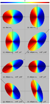 |
Fig. 1. Projected velocity field for some toy models with angle i, j (the kinematic axis is shown as a dashed line, the projected major axis is a solid line). Panel a: projection onto the plane of the sky of an observer with (i = 45 ° ,j = 0°) of disk with purely circular motion. Panel b: as in panel a but for a disk with purely radial velocities. Panel c: as in panel a but for an ellipse with purely circular motions. Panel d: as in panel c but for i = 45 ° ,j = 30°. Panel e: as in panel c but for i = 45 ° ,j = 60°. Panel f: as in panel c but for an ellipse with purely radial motions. Panel g: as in panel f but for i = 45 ° ,j = 30°. Panel h: as in panel f but for i = 45 ° ,j = 60°. |
Let us now consider the case of an ellipse with purely solid-body circular motions: Figs. 1c–e show three examples with parameters i = 45° and j = 0 ° ,30 ° ,60°. The ellipse has a flatness parameter
 (3)
(3)
where amax, amin are the intrinsic major and minor axes: as an illustrative case we take a relatively large value of the flatness parameter, that is, ι = 1. One may note that in this case the projected major axis forms angle ψ with the kinematic axis, where ψ = 90° for j = 0°; then it linearly decreases, becoming ψ = 0° for j = 90°. In Figs. 1f–h the case of an ellipse with purely radial motions are shown, for the same values of ι and i, j as before. In this case we find ψ = 0° for j = 0°; then ψ linearly increases with j, up to ψ = 90° for j = 90°. These simple exercises show that the relation between the kinematic and projected major axis, which occurs for a rotating disk, changes when the shape of the object is an ellipse; in particular, for an ellipse, ψ depends on the value of the angle j and the functional behavior of ψ(j) is relatively simple.
We can now introduce an additional, and crucial, feature of the velocity field. Indeed, in a physically motivated model of galaxy formation (see discussion below) it is quite natural that radial velocities are oriented outwards and are correlated with the major axis of the system. For this reason the kinematic axis is aligned with the projection of the major axis, which typically forms a small angle (i.e., ψ ≪ 90°) with the projected major axis. Thus, contrary to an ellipse with purely radial velocities, in this situation we expect that the kinematic axis and the major axis of the projected distribution forms, even for large values of j, a relatively small angle ψ, i.e., up to some tens of degrees.
Let us therefore consider a simple toy model that presents such a correlation. For instance, one possible way to assign this kind of nontrivial radial velocity is by fixing the 3D velocity field as
 (4)
(4)
where γ is an exponent that describes the strength of the correlation between radial velocities and the major axis of the ellipse, ω is the angle between r and the major axis, and A(r) is a function that describes the behavior of radial velocities as a function of the distance from the center. Figure 2 (upper left panel) shows the projection of such a toy model with ι = 1, γ = 2, and A(r) = 1 for certain values of the angles (i, j): one may note that, as expected, the angle ψ between the kinematic and the projected major axis is small and the same occurs for other values of (i, j). In order to investigate the behavior of the angle ψ as a function of the various parameters of this simple toy model, we have done several tests considering different values of ι, A(r) and γ and by considering several projection angles i, j. An example for ι = 1, A(r) = 1, γ = 0, 1, 2, 4, i = 45° and j = 45° is shown in Fig. 2: we find ψ ≈ 45° for γ = 0 (i.e., no correlation) and then it decreases when γ grows up to ψ ≈ 10° for γ = 4. Indeed, in the former case the alignment between the projected major axis and the kinematic axis is a consequence only of the ellipsoidal shape of the system. Instead, when γ grows the correlation between the direction of the radial velocity and the direction of the major axis gets stronger and therefore ψ decreases. Different values of the flatness parameter and of the projection angles change the value of ψ but not the trend with the correlation exponent γ.
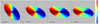 |
Fig. 2. Example of the angle between the projected major axis and the kinematic axis for an ellipse with ι = 1, A(r) = 1 for different values of the correlation exponent γ = 0, 1, 2, 4 (see Eq. (4)) for the case i = 45° and j = 45° (see text for details). |
Before concluding this series of simple toy models let us introduce a further element that may be relevant for the interpretation of the observations (see Sect. 3) and that is physically motivated, as we discuss in Sect. 4.4. We generate again a nonaxisymmetric system but now this is dominated by circular velocities in its inner coronas and by radial velocities in the outer coronas (see Fig. 3a). As in the previous case, the orientation of radial velocities is correlated with the major axis of the system. In particular, we choose the toy galaxy to be an ellipse with ι = 1 with solid-body circular velocities in its inner region and radial velocities in its outer region, and we fix γ = 2 in Eq. (4). We note that (see Figs. 3b–d) (i) the kinematic axis corresponding to the velocity field in the outer coronas forms a small angle ψ with the projected major axis, as in the previous case (see Fig. 2); (ii) the kinematic axes of the inner and outer regions form an angle that depends on j, that is, it is not simply ≈90° as one would have naively guessed on the basis of Eq. (1); and (iii) the signature of the two different kinds of the velocity fields, that is, circular and rotational, is, in this case, clearly recognizable by looking at the orientation of the kinematic axes defined by the velocity field in the inner and outer coronas, respectively. It is interesting to note that for some values of j this simple model gives values of ψ of the order of a few tens of degrees, so that the two kinematic axes (i.e., the inner and the outer one) are oriented almost in an anti-parallel way: it is therefore possible, for example by changing the shape of the ellipse and by taking a larger value of the correlation exponent γ, to further reduce this angle.
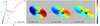 |
Fig. 3. Panel a: velocity profile of the toy model with rotational (vc) and radial (vr) velocities in the inner and outer coronas, respectively. Panels b–d: projected velocity field for different values of the angles i, j. The kinematic axis in the inner region is shown as a solid line and the kinematic axis in the outer region is shown as a dashed line. |
3. Modeling the two-dimensional velocity fields of a galaxy
In this section we first briefly review the standard methods for characterizing the observed two-dimensional velocity field of a galaxy under the assumption of axisymmetry, that is, the RDM and the RTRM, and for the detection of noncircular motions. We then consider the case of a nonaxisymmetric system and we introduce the REM, discussing its main features. Finally, we consider how to generalize the REM in a physically motivated way.
3.1. The rotating disk and tilted-ring models
As mentioned above, observations of galaxy velocity fields have been interpreted to support, at least to first order, the picture that disk galaxies are essentially axisymmetric systems in concentric circular rotation in a plane about a central axis. The velocity of this rotation, that is, the rotation curve, varies with the radius from the galactic center, and is assumed to be determined by the radial distribution of mass within the galaxy. This situation occurs if emitters move in an axisymmetric plane and on stable closed orbits, that is, on stationary circular orbits. Given this situation, the natural template employed to fit an observed velocity field is a disk with circular velocities such as those measured along the kinematic axis of the projected image of a real galaxy; in order to find the best RDM one minimizes the residuals, that is, the difference between real and model velocities, with respect to the inclination angle i. The residuals map traces noncircular (e.g., radial, random, nonplanar, etc.) motions. Therefore, in this case there is a single free parameter, the inclination angle, to be determined by the minimization procedure: others inputs from the observations are the systemic velocity and the angular coordinates of the center of the galaxy. In addition, to further characterize the orientation of a galaxy, the position angle of the galaxy major axis is usually determined, measured from north through east: however this angle does not necessarily enter into the minimization procedure.
A refinement of this method is the so-called RTRM, introduced by Begeman (1989) for the case of HI observations, but that of course can be generalized to other kinds of emitters. This assumes that a galaxy, again treated as an axisymmetric system, can be described as a set of concentric rings where each ring is characterized by a fixed value of the HI surface density, of the circular velocity vc(r), and of the orientation angles (i.e., the inclination angle i and position angle of the galaxy observed major axis ϕ6). The three ring parameters vc, i, and ϕ are solved through an iterative procedure and appropriate algorithms have been developed to this aim: for instance, within the GIPSY package (Groningen Image Processing SYstem; see van der Hulst et al. 1992) there is a routine that fits a set of so-called-tilted rings to the velocity field of a galaxy. The code fits a circular model to the velocity field by adjusting the ring parameters (namely, the kinematic centre, the inclination, the position angle, and the systemic velocity), so as to have a list of ring parameters as a function of radius. All the ring parameters are simultaneously fitted with a general least-squares fitting routine7.
3.2. The radial ellipse model
The radial ellipse model (REM) has, by construction, the three main characteristics of the class of nonaxisymmetric toy models illustrated in Fig. 2 and with velocities as in Eq. (4) (and that are common to the class of objects formed in the gravitational collapse of isolated self-gravitating cloud of particles; see discussion in Sect. 4.4); (i) it hypothesizes a nonaxisymmetric system where (ii) its velocity field in the outermost regions is dominated by radial motions such that (iii) radial velocities are correlated with the system major axis. The radial velocities are taken to be directed outwards (as noted above, the observed velocity field is symmetrical with respect to a change of sign and thus we could take radial inwards velocity as well and consider a rotation of 180° of the projected image). The REM must be minimized with respect to four parameters: the two angles i, j (see above for definitions), the flatness parameter of the ellipse ι (Eq. (3)), and the correlation exponent γ (Eq. (4)). In addition, as for the RDM, other inputs that must be determined from the observations are the systemic velocity and the angular coordinates of the center of the galaxy.
In this situation the residuals between the model and the observed velocity fields trace nonradial (e.g., circular, random, etc.) motions. Of course the REM is just a very rough template of the class of objects with the three characteristics discussed above: however it is sufficiently simple and versatile to allow a reasonably good fit of both simple toy models with a priori assigned properties and observed galaxy velocity fields. For what concerns the latter, our primary goal is to illustrate that a simple template, with a completely different velocity field than a rotating disk, is able to fit the data as well as the standard RDM that is usually employed.
The physical motivation for introducing the REM is that it captures the kinematical properties of a simple class of objects formed through the gravitational collapse of an isolated cloud of particles that initially breaks spherical symmetry. However these systems are not only dominated by radial motions in their outer parts but they are also generally characterized by having an inner region where instead rotational motions are predominant (see discussion in Sect. 4.4). In this situation it is possible to introduce a simple refinement of the REM, namely a combination of the REM and of the RDM.
Namely, in the outer parts of the system the velocity field is fitted by a REM while the inner parts, closer to axisymmetry, are fitted by a RDM. It is therefore possible to take into account, in a very simple way, the heterogeneous nature of the velocity field of this class of systems. The toy model illustrated in Fig. 2 encodes the properties of the joint model RDM+REM. The manner in which the motions change from being circular-dominated to radial-dominated as a function of the distance from the center of the galaxy can then be optimized for each galaxy and this is of course quite complicated to do for a general case. Below we consider an illustrative example of a THINGS galaxy where the transition between circular and radial motions is assumed to be a simple step function.
4. Two-dimensional velocity fields of THINGS galaxies
4.1. The data
The THINGS survey is a high spectral and spatial resolution survey of HI emission of 34 nearby galaxies obtained using the NRAO Very Large Array (Walter et al. 2008). The HI disks are better suited than optical emission to study galaxy kinematic as they allow an entire 2D mapping of the velocity field. In addition, while in the past HI images of galaxies lack angular resolution, this survey has a much higher resolution, making it a unique sample for the study of galaxy kinematics. Indeed, in order to determine for instance local motions within the disks of galaxies induced by substructures, one needs to resolve the size scales associated with features that cause these motions, such as bars, spiral arms, and oval distortions.
In order to measure high-precision rotation curves de Blok et al. (2008) considered a sub-sample of 19 galaxies from which they excluded galaxies with a low inclination (i.e., i < 40°) to avoid large uncertainties in the de-projected rotational velocity, tidally disturbed galaxies, and those galaxies with an inhomogeneous and anisotropic velocity field.
We note that the inclination angle can generally be measured under the assumption that a galaxy is a disk. In this way the inclination angle of a very nonaxisymmetric object may be overestimated: simply put, a high inclination galaxy for a RDM corresponds to a very prolate galaxy in the framework of a REM. For this reason, in addition to the de Blok et al. (2008) sub-sample, we have considered a further 9 galaxies with estimated (under the assumption mentioned above) inclination angle i < 40°. In addition, we have included in the sample some galaxies (e.g., NGC 3077, NGC 4449, NGC 5194) that have strong tidal interactions with neighboring galaxies. As we show below, all the galaxies that we considered, except NGC 5194 that has a very peculiar velocity field, show similar properties from the point of view of the fitting of their 2D velocity field with a RDM or with a REM.
4.2. Fitting the two-dimensional velocity field
In order to make the fit with a RDM or with a REM, each galaxy was coarse-grained with a grid of 64 × 64 equally sized cells and the residuals between the observations and the best fits were computed on such a grid. To find the best-fitting RDM or REM, we need to determine the best fitting parameters, that is, the inclination angle i for the RDM and i, j, γ, ι for the REM. We do this by minimizing the residuals between the model, computed for generic values of the parameters, and the actual data on each grid cell. To do so we compute first, for each grid cell, labeled by α and centered on projected coordinates  , the polar coordinates as defined above (see Eq. (2)):
 (5)
(5)
Subsequently, for the case of the RDM, we fix the value of the inclination angle i (the inclination angle was varied between 20° and 70° with Δi = 1) and we use Eq. (1) (with vR = 0) to compute the LOS velocity of the rotational model, denoted as  . We note that in the case where the unprojected size of the galaxy is larger than the maximum distance at which the LOS velocity profile extends, we perform a linear fit over the last five points of vlos(R) and then extrapolate using this fit to a higher radius. Finally, in order to get the best-fitting inclination angle, we minimize the sum of the residuals in all the cells with respect to i:
 (6)
(6)
where for the RDM  8.
8.
For the REM case, the angle i was varied in the range between 20° and 70° and j in the range between 20° and 70° and between 110° and 160° with a resolution of Δi = Δj = 10°. In addition the flatness parameter ι was varied in the range [0.3, 0.9] with Δι = 0.3 and the exponent γ in the range [1,6], but constrained to assume the values 1, 2, 4, 6. As the model is determined by four parameters, the numerical accuracy with which we can determine their values must be lowered. In particular, given this choice of parameters, each galaxy is compared with about 1000 templates. For each set of values of the parameters we numerically calculate the projection onto the sky with the same procedure as that used for the analysis of the toy models discussed in Sect. 2 and we coarse grain such an image; we then compute the value of the velocity  in each coarse-grained cell and we minimize again Eq. (6), where in this case
  .
.
We produced RTRM fits of the sample galaxies with kinemetry (Krajnović et al. 2006) to extract the axial ratio, q, and the position angle, ϕ, as a function of the radius. For each radius, kinemetry first produces the Fourier expansion of the velocity along elliptical coronas. We set the code to make the calculations for a grid of 11 × 11 coronas with axial ratios between q = 0.2 and q = 1.0 and position angles between ϕ = −90° and ϕ = 90°. The grid point, for which the  sum is minimized9, is used as a starting point for a Levenberg–Marquardt least-squares minimization from which a final q and ϕ are obtained. The reason for the choice of the function to be minimized is that errors in q increase b3 whereas errors in ϕ increase a1, a3, and b3. The radii for which the fits were done are the kinemetry default ones and follow the formula
 (7)
(7)
where R is the radius expressed in pixels and n are the non-negative integers. We made kinemetry to stop fitting once it reached a radius where velocity data are available for less than 50% of the data points.
As an illustrative example in Fig. 4 we show the determination of the best-fitting RTRM for the toy model discussed in Fig. 2, namely an ellipse with only radial motions correlated with the orientation of the major axis. One may note that the RTRM gives a very good representation of the radial velocity field with residuals smaller than 20% of the maximum velocity. This result shows the possible confusion between radial and rotational motion that may occur in the case of nonaxisymmetric systems when radial motions are dominant in the system.
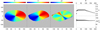 |
Fig. 4. Best fit RTRM (left panel) and residuals (right panel) for the toy model shown in Fig. 2 for γ = 2, i = 45°, and j = 70° (see text for details). |
4.3. Results
In Table 1 we summarize the results of the best fits for the THINGS galaxies. The best-fit inclination angle i for the RDM is reported in column (3); column (4) reports the amplitude of the residuals defined as
 (8)
(8)
Parameters and characteristics of the sample of THINGS galaxies considered in the analysis.
where σres is the variance of the best-fitting residual field, and σv is the variance of the observed velocity field. We note that both the residual and the velocity field (where, as mentioned above, we have subtracted the systemic velocity10) have zero expected mean and fres < 1 (in Table 1 this is reported as a percentage).
To quantify noncircular motions, we have computed the cumulative distribution function of the residuals and have adopted the value of 95% of the distribution of the residual velocities (in absolute value) as a representative value of the overall noncircular ( for the RDM) motion. Similarly, we report the best-fit parameters of the REM (i, j, ι, γ), the amplitude of the residuals defined as in Eq. (8) but using the REM best-fit template, and the value of 95% of the distribution of the residual velocities (in absolute value) as a representative value of the overall nonradial (
 for the REM) motions. Finally we report respectively
  and
and  for the RTRM.
In Figs. 5 and 6 we show the velocity maps for the best fitting velocity field and the corresponding residuals maps obtained with the RDM and with the REM for two representative examples (see Figs. A.1–A.25 for all the other galaxies)11.
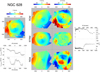 |
Fig. 5. NGC 628. Left panels: observed velocity profile (upper panel) and the velocity profile along the kinematic axis and along the axis orthogonal to it (bottom panels). The color-code of the velocity and residual fields is given in km s−1, where the systemic velocity of the object has been subtracted. Center panels from top to bottom: rotating disk model (RDM) velocity field (left), residual fields (right). Same as above but for the rotating tilted-ring model (RTRM) and radial ellipse model (REM). Right panels: axial ratio (upper panel) and the position angle as a function of the distance from the center (bottom panel). |
In addition, the 1D velocity profile is measured along two orthogonal slits: one aligned parallel to the kinematic axis and the other orthogonal to this direction (see Figs. 5 and 6 for two illustrative examples and Figs. A.1–A.25 for all the galaxies).
We find that the residuals of the RDM and of the REM are of the same order of magnitude, that is,  . As expected, both are larger than the residuals of the RTRM
  ; a similar situation occurs for
  ,
,  and
and  . When the 1D velocity profile along the kinematic axis is symmetrical, the 1D velocity profile along the axis orthogonal to the kinematic one has typically a small amplitude (e.g., DDO 154, NGC 2403, NGC 3351, etc.). In this situation the residual field has small amplitude and typically does not present any symmetric (with respect to the center of the galaxy) patterns. On the other hand, when the residual field has a large enough amplitude, that is,
  % (as for instance, NGC 628, NGC 925, NGC 2366, NGC 2976, etc.) then the 1D profile along the axis orthogonal to the kinematic one typically shows a large gradient with localized coherent patterns, that may correspond to particular structures (e.g., bar) of the object.
There are two kinds of velocity fields: those that show coherent patterns in the residuals field of the RDM and REM best fits, and those that do not. In the first case (e.g., NGC 2403) the overall kinematic axis well describes the system at all radii, while in the second case (e.g., NGC 628) this depends on the distance from the center. This same situation corresponds, in the RTRM, to a position angle ϕ showing a radius-dependent behavior. For example, the case of NGC 628 appears as a paradigmatic case in which the kinematic axis of the inner region is almost orthogonal to that of the outer region. Correspondingly the position angle of the RTRM shows a large variation, almost a step function behavior, as a function of radius. As discussed above (see Fig. 3), such a situation is compatible with the presence of two kinds of velocity fields, namely rotational in the inner part and radial in the outer part. A behavior similar to that shown by NGC 628 is present in several other galaxies and most notably NGC 3184, NGC 4214, NGC 4826, NGC 5236, NGC 6946, NGC 7793, and IC 2574.
As we discussed above, in order to take into account the complexity of galaxy velocity fields a single template with radial velocities may not be sufficient. Therefore we have considered, as a simple example and only for illustrative purposes, a template where at small distances from the center the system is dominated by circular motions and at large distances it is dominated by radial motions and is not axisymmetric. Therefore, in practice we have fitted the inner part with a RDM and the outer part with a REM, where the transition between circular and radial motions has been taken to be a step function. Of course it is possible to speculate that a smoother transition would give a better fit to the data, but this would clearly be very complicated implement and goes beyond the scope of the present work. For example, in the case of NGC 628 at about 270 arcsec the position angle makes a step from a value of about ϕ ≈ 20° to ϕ ≈ 90° (see Fig. 5). We thus obtain that the inner part is very well fitted by a RDM while the outer part can be fitted by a REM with a reasonably good accuracy (see Fig. 7) although the RTRM fit still provides a better fit.
 |
Fig. 7. Residuals resulting from a fit with a RDM (inner part) and a REM (outer part) to the galaxy NGC 628 (see text for details). |
It is therefore interesting to consider the case of NGC 4826, which seems to show a counter-rotating disk: the phenomenon of counter rotation (see, e.g., Bertola et al. 1999; Khoperskov & Bertin 2017) occurs when kinematic axes at different radii are oriented in an anti-parallel way. As discussed above, this situation can arise when there are two different kinds of velocity fields (i.e., a rotating one in the inner regions and a radial in the outer ones) in a nonaxisymmetric object (see Fig. 3) and a modeling with a RDM+REM is therefore possible. Alternatively, it is possible to consider a situation where there are only radial velocities which are however oriented in different directions in the inner and outer parts of the object; for example the inner radial velocity field is directed inwards and the outer outwards, thus giving rise to patterns in the velocity field that can be confused with the phenomenon of counter rotation.
4.4. Discussion
As mentioned above, our aim in this work is not to discuss the properties of the observed velocity field of each galaxy in detail, but rather to discuss the method used to determine circular and radial motions from the data and to show that one can arrive at very different conclusions depending on the set of hypotheses on which a fitting model is based. In particular, we have discussed the role of the crucial hypotheses, usually adopted, of axisymmetry and circular motions. These are based on a galaxy model, where stars and other emitters move in almost circular and stationary orbits in a disk, with or without a warp, around the galactic center.
Instead, the main dynamical elements that have inspired the REM are characteristic of a different dynamical model of spiral galaxies that has emerged from simple simulations of isolated and rotating overdensities of self-gravitating particles. (Benhaiem et al. 2017, 2018). In this case, the combination of an initial rotational motion with a strong collapse, which occurs for an isolated system driven by its own mean-field gravitational potential, leads very naturally to transients, like spiral arms, which have a complex coherent spatial distribution and bear a striking qualitative resemblance to the real spiral galaxies. The lifetime of these transients can be large compared to the system’s characteristic time scale τd ≈ 1/-pagination  , but smaller than the collisional time scale τcoll, that is, these transients appear in a range of time τd ≪ t ≪ τcoll before the system reaches a truly virialized state. As discussed in Benhaiem et al. (2017) the physical units can be normalized by fixing the typical velocity ≈200 km s−1 and the typical mass ≈1011 M⊙: in this situation one obtains a reasonable size for the object, namely of the order of tens of kiloparsecs if the collapse process that generated the disk and arms occurred much more recently (i.e., on a time-scale of the order of 1 Gyr) than the formation of the oldest stars in these galaxies (with an age ∼10 Gyr). The precise normalization depends however on the properties of the initial conditions, as the amplitude of radial velocities and the size of the system can greatly vary according to both the amplitude of the normalized spin parameter and the shape of the initial conditions (Benhaiem et al. 2018).
In these systems, the origin of the spiral-like arms is related to the initial breaking of spherical symmetry and to the nonzero initial angular momentum. Indeed, if the evolution leads to a sufficiently strong contraction of the system during the collapse, some particles may gain some kinetic energy in the form of a radial velocity oriented outwards, which adds to the initial rotational velocity. These are the particles that are initially placed at the largest distance from the origin; the dynamical mechanism associated with the monolithic collapse of the cloud thus amplifies the initial deviations from spherical symmetry and generates radial motions correlated with the longest axis of the system. The particles which gain the largest amount of energy will travel, once faraway from the center of the system, in a gravitational potential which, to a crude approximation, is spherically symmetric and stationary; thus, because of approximate conservation of angular momentum, their radial displacement will be correlated with a decrease of their angular velocity relative to the center of the structure. As a result the particles which go furthest will have a smaller angular velocity than those closer to the center, and will therefore “wind up” less and a spiral-type structure can result. Briefly, the outermost particles of the system that is formed after the collapse are loosely bound, or are possibly even free particles and have predominantly radial velocities directed outwards, although they still have a non-negligible fraction of their velocity in a rotational component. On the other hand, the system’s collapse is generally strong enough to form an almost virialized and triaxial core with an isotropic velocity dispersion. In addition, in an intermediate region between the inner core and the outer loosely bound particles a flat disk-like configuration is formed where rotational motions are predominant. Thus, the velocity field that results from these simple systems is heterogeneous in nature and strongly scale dependent.
It must be emphasized that the class of models considered by Benhaiem et al. (2017, 2018) is very simplistic, not just because of the idealization of the initial conditions but also in that it neglects everything but gravitational dynamics. Any detailed quantitative model of a real galaxy will of course necessarily need to consider more complex initial conditions and also incorporate nongravitational physics, such as gas dynamics, cooling, star formation, and so on. In this respect we note that in standard models of galaxy formation the key element in the formation of a disk galaxy is the dissipation associated with nongravitational processes. Instead, in the purely gravitational simulations by Benhaiem et al. (2017, 2018) disk-like configurations with transient spiral arms are formed by purely dissipationless gravitational dynamics if the initial conditions break spherical symmetry. For this reason, a more complete study of this class of models requires the study of hydrodynamical simulations of nonaxisymmetric systems: this is currently an ongoing work (Sylos Labini et al., in prep.).
For what concerns the problem of cosmological galaxy formation, the monolithic collapse of an overdensity may occur in top-down structure formation scenarios like warm dark-matter models. This process, depending on the properties of the power-spectrum of density fluctuations, can be theoretically approximated by the gravitational collapse of an isolated cloud (Peebles 1980) similar to what occurs in the simulations of a cold collapse.
To summarize, the main features of the outermost region of these systems are: (i) they are not axisymmetric, (ii) they have a radial velocity field directed outwards that (iii) has a strong correlation with the direction of the major axis of the system. These are three features that are encoded in the REM. In addition, this class of system usually presents an extended flattened region which rotates coherently about a well virialized core of triaxial shape with an approximately isotropic velocity dispersion. For this reason the resulting velocity field has a heterogeneous scale-dependent behavior and a fitting model that assumes only a single type of velocity field (rotational or radial) is not suitable to describe the systems at all radii.
5. Conclusions
Observed 2D galaxy velocity maps are usually interpreted under the hypothesis that stars (and other emitters) move in an axisymmetric disk and in stationary circular orbits around the galactic center. This hypothesis is corroborated by the observed velocity gradient in such maps, that is, at least at first order, consistent with a rotational velocity field. In order to characterize galactic kinematics in greater detail, these 2D velocity maps are fitted to a rotating disk model (RDM) or, in order to take into account the possible presence of a warp in the galaxy, to a rotating tilted-ring model (RTRM). In both cases, the hypothesis used is that the galaxy is axisymmetric and that stars and other emitters move in circular orbits: in the case of the RTRM it is also assumed that circular orbits at different distances from the galaxy’s center have different inclination. The residuals, that is, the difference between the observed and the model velocity fields, are then interpreted to trace noncircular motions like radial, random, and other motions.
In this paper we have shown that if the system is not assumed to be axisymmetric then it is possible to elaborate a different interpretation of the observed 2D galaxy velocity maps. This is based on a different dynamical model of the outermost regions of the observed galaxies: namely that stars and other emitters have a velocity field where radial motions are large and/or dominant. Such a model describes the properties of the transient spiral-like structures that are formed in the collapse of isolated, initially nonspherical, and rotating clouds of particles in which is generically formed a rotating disk surrounded by transient spiral-like arms of which the motion is mainly radial. The complex velocity and configurational properties of these structures can be, as a first rough approximation, described as an ellipse with radial velocities directed outwards whose amplitude is correlated with the major axis of the ellipse. These properties are encoded in the fitting model that we have described, the radial ellipse model (REM).
We have shown that, from a numerical point of view, for a sub-sample of galaxies extracted from the THINGS data, the REM works as well as the RDM; that is residuals are of the same order of magnitude both for the case in which the fitting template is a disk with circular velocities (RDM) and the case of an ellipse with radial velocities correlated with the major semi-axis (REM). It should be noted that the REM is defined by four parameters rather than only one, as in the RDM. This is because the former describes a system (i.e., an ellipse with a correlation between the direction of radial velocities and its major axis) that is much more complicated than a simple disk with only circular motions. Thus, from a purely mathematical analysis point of view, given that the REM and RDM give similar residuals, if we apply the Akaike information criterion (Akaike 1974), the REM has a likelihood smaller by a factor of ∼exp(−6) compared to that for the RDM, and therefore is much less favorable. However, although the RDM delivers the best results compared to the number of parameters used, it does not take into account the possible complexities of real galaxies, such as the fact that axisymmetry is often observed to be broken.
We have also studied the best fits obtained with the RTRM and found that in this case the residuals are the smallest. However we have argued that this is possible because such a model allows a radius-dependent orientation of the kinematic axis and that, in this way, it may confuse rotational and radial motion, if they are present at different radii in a given system. Finally we have stressed that, in order to more accurately describe a heterogeneous and scale-dependent velocity field, a template consisting in a combination of the RDM and the REM may be more suitable. This joint template represents an alternative physically motivated model to the RTRM, able to characterize the velocity fields in nonaxisymmetric systems. In this respect we stress that the presence of the warp, confirmed in several cases by observations different from kinematical ones (Sancisi 1976; Reshetnikov & Combes 1998; Schwarzkopf & Dettmar 2001; García-Ruiz et al. 2002; Sánchez-Saavedra et al. 2003; Levine et al. 2006; Kalberla et al. 2007; Reylé et al. 2009), is not incompatible with the presence of radial motions: that is, the presence of a warp does not imply, but it is only compatible with, the key assumption of the RTRM that stars orbit on circular orbits with a different inclination as a function of the distance from the galaxy’s center.
It is clear that when the mass is weakly bound or even unbound, as occurs when radial velocities are not negligible, one greatly overestimates the actual enclosed mass from the dynamical mass Mdyn(r)≈v2(r)⋅r/G, that is, if one assumes stationary circular orbit. Specifically, if a part of the observed velocity has a contribution from a radial component, and thus the system has not reached a truly virialized state, then Mdyn(r) gives a greater estimation of the actual mass: this situation suggests the possibility that observed velocity curves of external galaxies might require much less dark matter than what is usually estimated from Mdyn(r) if the outer parts of the galaxy are far from stationary and the motions are predominantly radial and spatially correlated in a nonaxisymmetric distribution, rather than rotational (Benhaiem et al. 2017).
Concomitantly, as we have shown, in external galaxies it is not straightforward to disentangle between rotational and radial velocity fields if the system is not axisymmetric; for our own Galaxy the measurement of the radial and tangential components of stars’ velocities is now possible with an increasing precision. In this respect, it is interesting to mention that, while it has been known for several decades that the Galactic disk contains large-scale nonaxisymmetric features, a complete understanding of these asymmetric structures and of their velocities fields is still lacking. The recent Gaia DR2 maps (Gaia Collaboration 2018) have clearly shown that the Milky Way is not an axisymmetric system at equilibrium, but that it is characterized by streaming motions in all the three velocity components. In particular these data have confirmed the coherent radial motion in the direction of the anti-center, earlier detected up to 16 kpc by López-Corredoira & González-Fernández (2016) and recently extended up to 20 kpc by López-Corredoira et al. (2018).
At larger distances, even though the data are very noisy, using a statistical method of deconvolution of the parallax errors, López-Corredoira & Sylos Labini (2019) were able to measure not only significant departures of circularity in the mean orbits with radial Galactocentric velocities between −20 and +20 km s−1 but also vertical velocities between −10 and +10 km s−1, variations of rotation speed with position, and asymmetries between northern and southern Galactic hemisphere of up to 20 kpc. Of course the tangential velocity component is still very much larger than the radial one, and this latter can already have an important dynamical effect (López-Corredoira et al. 2018). For this reason it is crucially important to study the kinematics of our Galaxy in the outermost region of the disk. The next Gaia data release, foreseen for 2020, with improved astrometry and photometry allowing it to map the velocity field in the outer part of the Galactic disk, will be able to map distances larger than r > 20 kpc.
The kinematic axis is the axis passing through the center of mass of the distribution and along which the difference of the observed velocities at the two extreme points is maximal.
The inclination angle is the angle between the LOS of the observer and a vector orthogonal to the plane of the disk.
With respect to the systemic velocity of the galaxy.
In reality it is a 3D object with thickness much smaller than its main linear dimensions.
Of course the observed velocity map is symmetrical with respect to a change of sign in the velocity field: i.e., if we take radial velocities directed inwards rather than outwards observationally the system is the same modulo a rotation of 180°. The same occurs for all toy models discussed below and also for the REM. However, from a physical point of view a radial velocity field directed outwards is expected in some models of galaxy formation as we discuss in what follows.
We adopt the standard convention according to which the position angle of the galaxy major axis is measured from north through east (Beckman et al. 2004).
We note that the GIPSY task ROTCUR has also the option of computing radial motions that describes, for a disk, the second term in Eq. (1).
We note that the value of the position angle of the galaxy major axis is irrelevant for the minimization of Eq. (6) and is therefore not reported. In addition, in the RDM the center of the galaxy image is computed by considering only the inner pixels.
a1, a3, and b3 are the sin (ϕα), sin (3ϕα), and cos (3ϕα) coefficients of the Fourier expansion, respectively.
The systemic velocity for the de Blok et al. (2008) sample is reported in their Table 2, for the other 9 galaxies we have estimated it as the velocity of the center. We note that this information enters as an overall normalizing factor in the velocity scale.
In all figures the radius is expressed in pixels.
Acknowledgments
FSL and DB thank Michael Joyce for collaborations and discussions, and Roberto Capuzzo Dolcetta for useful comments. This work was granted access to the HPC resources of The Institute for scientific Computing and Simulation financed by Region Ile de France and the project Equip@Meso (reference ANR-10-EQPX- 29-01) overseen by the French National Research Agency (ANR) as part of the Investissements d’Avenir program. MLC was supported by the grant AYA2015-66506-P of the Spanish Ministry of Economy and Competitiveness (MINECO). We acknowledge the use of the THINGS project data available at http://www.mpia.de/THINGS/Data.html. We thank Fabian Walter for kindly giving us access to the data of IC 2574. We acknowledge the use of the code kinemetry by Krajnović et al. (2006). Finally we thank an anonymous referee for very useful comments and suggestions.
References
- Akaike, H. 1974, IEEE Trans. Autom. Control, 19, 716 [NASA ADS] [CrossRef] [MathSciNet] [Google Scholar]
- Baldwin, J. E., Lynden-Bell, D., & Sancisi, R. 1980, MNRAS, 193, 313 [NASA ADS] [CrossRef] [Google Scholar]
- Beckman, J. E., Zurita, A., & Vega Beltrán, J. C. 2004, Lecture Notes and Essays in Astrophysics, 1, 43 [NASA ADS] [Google Scholar]
- Begeman, K. G. 1987, PhD Thesis, Kapteyn Institute [Google Scholar]
- Begeman, K. G. 1989, A&A, 223, 47 [NASA ADS] [Google Scholar]
- Benhaiem, D., Joyce, M., & Sylos Labini, F. 2017, ApJ, 851, 19 [NASA ADS] [CrossRef] [Google Scholar]
- Benhaiem, D., Sylos Labini, F., Joyce, M., et al. 2018, Phys. Rev. E, in press [Google Scholar]
- Bertola, F., & Corsini, E. M. 1999, in Galaxy Interactions at Low and High Redshift, eds. J. E. Barnes, & D. B. Sanders, IAU Symp., 186, 149 [NASA ADS] [CrossRef] [Google Scholar]
- Bosma, A. 1981, AJ, 86, 1825 [NASA ADS] [CrossRef] [Google Scholar]
- de Blok, W. J. G., Walter, F., Brinks, E., et al. 2008, AJ, 136, 2648 [NASA ADS] [CrossRef] [Google Scholar]
- Erroz-Ferrer, S., Knapen, J. H., Font, J., et al. 2012, MNRAS, 427, 2938 [NASA ADS] [CrossRef] [Google Scholar]
- Erroz-Ferrer, S., Knapen, J. H., Font, J., & Beckman, J. E. 2015, Highlights of Astron., 16, 328 [NASA ADS] [Google Scholar]
- Gaia Collaboration (Katz, D., et al.) 2018, A&A, 616, A11 [NASA ADS] [CrossRef] [EDP Sciences] [Google Scholar]
- García-Ruiz, I., Kuijken, K., & Dubinski, J. 2002, MNRAS, 337, 459 [NASA ADS] [CrossRef] [Google Scholar]
- Jog, C. J., & Combes, F. 2009, Phys. Rep., 471, 75 [NASA ADS] [CrossRef] [Google Scholar]
- Jorsater, S., & van Moorsel, G. A. 1995, AJ, 110, 2037 [NASA ADS] [CrossRef] [Google Scholar]
- Kalberla, P. M. W., Dedes, L., Kerp, J., & Haud, U. 2007, A&A, 469, 511 [NASA ADS] [CrossRef] [EDP Sciences] [Google Scholar]
- Khoperskov, S., & Bertin, G. 2017, A&A, 597, A103 [NASA ADS] [CrossRef] [EDP Sciences] [Google Scholar]
- Kornreich, D. A., Haynes, M. P., Lovelace, R. V. E., & van Zee, L. 2000, AJ, 120, 139 [NASA ADS] [CrossRef] [Google Scholar]
- Krajnović, D., Cappellari, M., de Zeeuw, P. T., & Copin, Y. 2006, MNRAS, 366, 787 [NASA ADS] [CrossRef] [Google Scholar]
- Laine, S., Knapen, J. H., Muñoz-Mateos, J.-C., et al. 2014, MNRAS, 444, 3015 [NASA ADS] [CrossRef] [Google Scholar]
- Levine, E. S., Blitz, L., & Heiles, C. 2006, ApJ, 643, 881 [NASA ADS] [CrossRef] [Google Scholar]
- López-Corredoira, M., & González-Fernández, C. 2016, AJ, 151, 165 [NASA ADS] [CrossRef] [Google Scholar]
- López-Corredoira, M., & Sylos Labini, F. 2019, A&A, 621, A48 [NASA ADS] [CrossRef] [EDP Sciences] [Google Scholar]
- López-Corredoira, M., Sylos Labini, F., Kalberla, P. M. W., & Allende Prieto, C. 2018, AJ, submitted [Google Scholar]
- Oh, S.-H., de Blok, W. J. G., Walter, F., Brinks, E., & Kennicutt, Jr., R. C. 2008, AJ, 136, 2761 [NASA ADS] [CrossRef] [Google Scholar]
- Peebles, P. J. E. 1980, The Large-Scale Structure of the Universe (Princeton: Princeton University Press) [Google Scholar]
- Reshetnikov, V., & Combes, F. 1998, A&A, 337, 9 [NASA ADS] [Google Scholar]
- Reylé, C., Marshall, D. J., Robin, A. C., & Schultheis, M. 2009, A&A, 495, 819 [NASA ADS] [CrossRef] [EDP Sciences] [Google Scholar]
- Rix, H.-W., & Zaritsky, D. 1995, ApJ, 447, 82 [NASA ADS] [CrossRef] [Google Scholar]
- Rogstad, D. H., Lockhart, I. A., & Wright, M. C. H. 1974, ApJ, 193, 309 [NASA ADS] [CrossRef] [Google Scholar]
- Rubin, V. C. 1983, Science, 220, 1339 [NASA ADS] [CrossRef] [Google Scholar]
- Sánchez-Saavedra, M. L., Battaner, E., Guijarro, A., López-Corredoira, M., & Castro-Rodríguez, N. 2003, A&A, 399, 457 [NASA ADS] [CrossRef] [EDP Sciences] [Google Scholar]
- Sancisi, R. 1976, A&A, 53, 159 [NASA ADS] [Google Scholar]
- Schoenmakers, R. H. M., Franx, M., & de Zeeuw, P. T. 1997, MNRAS, 292, 349 [NASA ADS] [CrossRef] [Google Scholar]
- Schwarzkopf, U., & Dettmar, R.-J. 2001, A&A, 373, 402 [NASA ADS] [CrossRef] [EDP Sciences] [Google Scholar]
- Sellwood, J. A., & Sánchez, R. Z. 2010, MNRAS, 404, 1733 [NASA ADS] [Google Scholar]
- Sofue, Y., & Rubin, V. 2001, ARA&A, 39, 137 [NASA ADS] [CrossRef] [Google Scholar]
- Song, G.-X. 1983, Astron. Space. Sci., 95, 431 [NASA ADS] [CrossRef] [Google Scholar]
- Thonnard, N., Rubin, V. C., Ford, Jr., W. K., & Roberts, M. S. 1978, AJ, 83, 1564 [NASA ADS] [CrossRef] [Google Scholar]
- Trachternach, C., de Blok, W. J. G., Walter, F., Brinks, E., & Kennicutt, Jr., R. C. 2008, AJ, 136, 2720 [NASA ADS] [CrossRef] [Google Scholar]
- van der Hulst, J. M., Terlouw, J. P., Begeman, K. G., Zwitser, W., & Roelfsema, P. R. 1992, in Astronomical Data Analysis Software and Systems I, eds. D. M. Worrall, C. Biemesderfer, & J. Barnes, ASP Conf. Ser., 25, 131 [NASA ADS] [Google Scholar]
- van der Kruit, P. C., & Bosma, A. 1978, A&A, 34, 259 [NASA ADS] [Google Scholar]
- Walter, F., Brinks, E., de Blok, W. J. G., et al. 2008, AJ, 136, 2563 [NASA ADS] [CrossRef] [Google Scholar]
- Zurita, A., Relaño, M., Beckman, J. E., & Knapen, J. H. 2004, A&A, 413, 73 [NASA ADS] [CrossRef] [EDP Sciences] [Google Scholar]
Appendix A: Additional figures
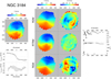 |
Fig. A.10. As in Fig. 5 but for NGC 3184. |
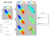 |
Fig. A.11. As in Fig. 5 but for NGC 3198. |
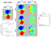 |
Fig. A.12. As in Fig. 5 but for NGC 3351. |
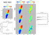 |
Fig. A.13. As in Fig. 5 but for NGC 3521. |
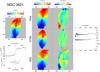 |
Fig. A.14. As in Fig. 5 but for NGC 3621. |
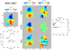 |
Fig. A.15. SAs in Fig. 5 but for NGC 3627. |
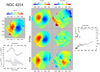 |
Fig. A.16. As in Fig. 5 but for NGC 4214. |
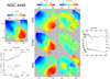 |
Fig. A.17. As in Fig. 5 but for NGC 4449. |
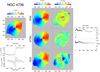 |
Fig. A.18. As in Fig. 5 but for NGC 4736. |
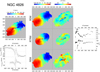 |
Fig. A.19. As in Fig. 5 but for NGC 4826. |
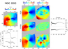 |
Fig. A.20. As in Fig. 5 but for NGC 5055. |
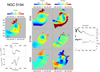 |
Fig. A.21. As in Fig. 5 but for NGC 5194. |
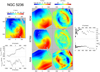 |
Fig. A.22. As in Fig. 5 but for NGC 5236. |
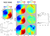 |
Fig. A.23. SAs in Fig. 5 but for NGC 6946. |
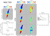 |
Fig. A.24. As in Fig. 5 but for NGC 7331. |
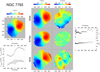 |
Fig. A.25. As in Fig. 5 but for NGC 7793. |
All Tables
Parameters and characteristics of the sample of THINGS galaxies considered in the analysis.
All Figures
|
Fig. 1. Projected velocity field for some toy models with angle i, j (the kinematic axis is shown as a dashed line, the projected major axis is a solid line). Panel a: projection onto the plane of the sky of an observer with (i = 45 ° ,j = 0°) of disk with purely circular motion. Panel b: as in panel a but for a disk with purely radial velocities. Panel c: as in panel a but for an ellipse with purely circular motions. Panel d: as in panel c but for i = 45 ° ,j = 30°. Panel e: as in panel c but for i = 45 ° ,j = 60°. Panel f: as in panel c but for an ellipse with purely radial motions. Panel g: as in panel f but for i = 45 ° ,j = 30°. Panel h: as in panel f but for i = 45 ° ,j = 60°. |
| In the text | |
|
Fig. 2. Example of the angle between the projected major axis and the kinematic axis for an ellipse with ι = 1, A(r) = 1 for different values of the correlation exponent γ = 0, 1, 2, 4 (see Eq. (4)) for the case i = 45° and j = 45° (see text for details). |
| In the text | |
|
Fig. 3. Panel a: velocity profile of the toy model with rotational (vc) and radial (vr) velocities in the inner and outer coronas, respectively. Panels b–d: projected velocity field for different values of the angles i, j. The kinematic axis in the inner region is shown as a solid line and the kinematic axis in the outer region is shown as a dashed line. |
| In the text | |
|
Fig. 4. Best fit RTRM (left panel) and residuals (right panel) for the toy model shown in Fig. 2 for γ = 2, i = 45°, and j = 70° (see text for details). |
| In the text | |
|
Fig. 5. NGC 628. Left panels: observed velocity profile (upper panel) and the velocity profile along the kinematic axis and along the axis orthogonal to it (bottom panels). The color-code of the velocity and residual fields is given in km s−1, where the systemic velocity of the object has been subtracted. Center panels from top to bottom: rotating disk model (RDM) velocity field (left), residual fields (right). Same as above but for the rotating tilted-ring model (RTRM) and radial ellipse model (REM). Right panels: axial ratio (upper panel) and the position angle as a function of the distance from the center (bottom panel). |
| In the text | |
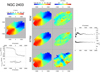 |
Fig. 6. As in Fig. 5 but for NGC 2403. |
| In the text | |
|
Fig. 7. Residuals resulting from a fit with a RDM (inner part) and a REM (outer part) to the galaxy NGC 628 (see text for details). |
| In the text | |
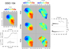 |
Fig. A.1. As in Fig. 5 but for DDO 154. |
| In the text | |
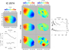 |
Fig. A.2. As in Fig. 5 but for IC 2574. |
| In the text | |
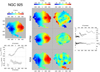 |
Fig. A.3. As in Fig. 5 but for NGC 925. |
| In the text | |
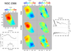 |
Fig. A.4. SAs in Fig. 5 but for NGC 2366. |
| In the text | |
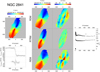 |
Fig. A.5. As in Fig. 5 but for NGC 2841. |
| In the text | |
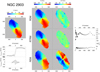 |
Fig. A.6. As in Fig. 5 but for NGC 2903. |
| In the text | |
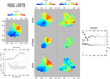 |
Fig. A.7. As in Fig. 5 but for NGC 2976. |
| In the text | |
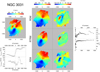 |
Fig. A.8. As in Fig. 5 but for NGC 3031. |
| In the text | |
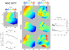 |
Fig. A.9. SAs in Fig. 5 but for NGC 3077. |
| In the text | |
|
Fig. A.10. As in Fig. 5 but for NGC 3184. |
| In the text | |
|
Fig. A.11. As in Fig. 5 but for NGC 3198. |
| In the text | |
|
Fig. A.12. As in Fig. 5 but for NGC 3351. |
| In the text | |
|
Fig. A.13. As in Fig. 5 but for NGC 3521. |
| In the text | |
|
Fig. A.14. As in Fig. 5 but for NGC 3621. |
| In the text | |
|
Fig. A.15. SAs in Fig. 5 but for NGC 3627. |
| In the text | |
|
Fig. A.16. As in Fig. 5 but for NGC 4214. |
| In the text | |
|
Fig. A.17. As in Fig. 5 but for NGC 4449. |
| In the text | |
|
Fig. A.18. As in Fig. 5 but for NGC 4736. |
| In the text | |
|
Fig. A.19. As in Fig. 5 but for NGC 4826. |
| In the text | |
|
Fig. A.20. As in Fig. 5 but for NGC 5055. |
| In the text | |
|
Fig. A.21. As in Fig. 5 but for NGC 5194. |
| In the text | |
|
Fig. A.22. As in Fig. 5 but for NGC 5236. |
| In the text | |
|
Fig. A.23. SAs in Fig. 5 but for NGC 6946. |
| In the text | |
|
Fig. A.24. As in Fig. 5 but for NGC 7331. |
| In the text | |
|
Fig. A.25. As in Fig. 5 but for NGC 7793. |
| In the text | |
Current usage metrics show cumulative count of Article Views (full-text article views including HTML views, PDF and ePub downloads, according to the available data) and Abstracts Views on Vision4Press platform.
Data correspond to usage on the plateform after 2015. The current usage metrics is available 48-96 hours after online publication and is updated daily on week days.
Initial download of the metrics may take a while.