| Issue |
A&A
Volume 622, February 2019
|
|
|---|---|---|
| Article Number | A183 | |
| Number of page(s) | 9 | |
| Section | Extragalactic astronomy | |
| DOI | https://doi.org/10.1051/0004-6361/201833547 | |
| Published online | 21 February 2019 | |
J-PLUS: Analysis of the intracluster light in the Coma cluster
1
Observatório Nacional, Rua General José Cristino, 77 – Bairro Imperial de São Cristóvão, Rio de Janeiro, 20921-400, Brazil
e-mail: This email address is being protected from spambots. You need JavaScript enabled to view it.
2
Instituto de Astrofísica de Andalucía, Glorieta de la Astronomía s/n, 18008 Granada, Spain
e-mail: This email address is being protected from spambots. You need JavaScript enabled to view it.
3
Department of Physics and Astronomy, University of Alabama, Box 870324, Tuscaloosa, AL 35487, USA
4
Department of Astronomy, University of Michigan, 311 West Hall, 1085 South University Ave., Ann Arbor, MI 48109-1107, USA
5
X-ray Astrophysics Laboratory, NASA Goddard Space Flight Center, Greenbelt, MD 20771, USA
6
Department of Physics, University of Maryland, Baltimore County, 1000 Hilltop Circle, Baltimore, MD 21250, USA
7
Departamento de Física, Universidade Federal de Sergipe, Av. Marechal Rondon s/n, 49000-000 São Cristóvão, SE, Brazil
8
Instituto de Astronomia, Geofísica e Ciências Atmosféricas, Universidade de São Paulo, Rua do Matão 1226, C. Universitária, São Paulo 05508-090, Brazil
9
Departamento de Astronomia, Instituto de Física, Universidade Federal do Rio Grande do Sul, Porto Alegre, RS, Brazil
10
Centro de Estudios de Física del Cosmos de Aragón, Unidad Asociada al CSIC, Plaza San Juan 1, 44001 Teruel, Spain
Received:
1
June
2018
Accepted:
28
September
2018
Abstract
Context. The intracluster light (ICL) is a luminous component of galaxy clusters composed of stars that are gravitationally bound to the cluster potential, but do not belong to the individual galaxies. Previous studies of the ICL have shown that its formation and evolution are intimately linked to the evolutionary stage of the cluster. Thus, the analysis of the ICL in the Coma cluster will give insights into the main processes driving the dynamics in this highly complex system.
Aims. Using a recently developed technique, we measure the ICL fraction in Coma at several wavelengths, using the J-PLUS unique filter system. The combination of narrow- and broadband filters provides valuable information on the dynamical state of the cluster, the ICL stellar types, and the morphology of the diffuse light.
Methods. We used the Chebyshev-Fourier intracluster light estimator (CICLE) to distinguish the ICL from the light of the galaxies, and to robustly measure the ICL fraction in seven J-PLUS filters.
Results. We obtain the ICL fraction distribution of the Coma cluster at different optical wavelengths, which varies from ∼7%−21%, showing the highest values in the narrowband filters J0395, J0410, and J0430. This ICL fraction excess is a distinctive pattern that has recently been observed in dynamically active clusters (mergers), indicating a higher amount of bluer stars in the ICL than in cluster galaxies.
Conclusions. The high ICL fractions and the excess in the bluer filters are indicative of a merging state. The presence of younger stars or stars with lower metallicity in the ICL suggests that the main mechanism of ICL formation for the Coma cluster is the stripping of the stars in the outskirts of infalling galaxies and possibly the disruption of dwarf galaxies during past or ongoing mergers.
Key words: galaxies: clusters: individual: Coma / techniques: image processing
© ESO 2019
1. Introduction
The Coma cluster (Abell 1656) is the most massive cluster nearby (z ∼ 0.023), with a virial mass of M200 = 1.88 × 10¹⁵ h−1 M⊙ (Kubo et al. 2007). Originally thought to be a classical example of a virialized cluster given its apparent spherical symmetry, compactness, luminosity segregation, and regularity (Zwicky 1957; Kent & Gunn 1982; Mellier et al. 1988), Coma now is known to be dynamically very active. It has two D galaxies near the center (NGC 4874 and NGC 4889), and its spatial distribution shows several subclumps and overdensities (Fitchett & Webster 1987; Mellier et al. 1988; Ulmer et al. 1994; Merritt & Tremblay 1994; Conselice & Gallagher III 1998; Mendelin & Binggeli 2017). Its galaxy velocity distribution presents evidence for substructures and departure from a single Gaussian, such as significant skewness and several peaks (Fitchett & Webster 1987; Merritt 1987; Kent & Gunn 1982; Mellier et al. 1988; Colless & Dunn 1996). Many substructures are also found in the elongated X-ray emission of Coma (whose peak is not coincident with any of the brightest cluster galaxies – BCGs), with a particularly relevant arc-like emission between the Coma core and the NGC 4839 group that is consistent with a bow shock (Johnson et al. 1979; Briel et al. 1992, 2011; Davis & Mushotzky 1993; White et al. 1993; Vikhlinin et al. 1997; Arnaud et al. 2001; Neumann et al. 2001, 2003). Coma has a high intracluster gas temperature (kT > 8 keV) and lacks significant temperature and metallicity gradients in X-rays within an angular radius of 30 arcmin ( kpc) from the cluster core (Edge et al. 1992; Watt et al. 1992; Colless & Dunn 1996; Arnaud et al. 2001; Simionescu et al. 2013). It also hosts a giant radio halo and a peripheral radio relic connected through a low-surface brightness ridge of emission (Willson 1970; Jafe et al. 1976; Giovannini et al. 1985; Kim et al. 1990; Venturi et al. 1990; Deiss et al. 1997; Kronberg et al. 2007; Brown & Rudnick 2011).
A formation scenario that is currently contemplated for the Coma cluster is a merger of two sub-clusters or groups associated with the two D galaxies, NGC 4874 and NGC 4889, possibly after their second core-crossing (Briel et al. 1992; Watt et al. 1992; Davis & Mushotzky 1993; Colless & Dunn 1996; Arnaud et al. 2001; Neumann et al. 2003; Adami et al. 2005b; Gerhard et al. 2007). Most dynamical and X-ray studies suggest that the group related to NGC 4874 could have been at the center of the main cluster potential in the past, being displaced out of the bottom of the potential well by the infall of the group associated with NGC 4889 (e.g., Davis & Mushotzky 1993; Colless & Dunn 1996; Gerhard et al. 2007). Moreover, analyses of X-ray substructures and radio emission indicate that this second subcluster is partially disrupted and has ejected NGC 4889 (Colless & Dunn 1996). Evidence also points to the presence of a third subcluster around NGC 4839 that would be currently merging into the main Coma cluster (Briel et al. 1992, 2011; Colless & Dunn 1996; Neumann et al. 2001, 2003; Adami et al. 2005b).
Zwicky (1957) was the first to report a diffuse intergalactic light in the core of the Coma cluster, detected by direct photography, to be later confirmed by Gunn (1969) using photoelectric drift-scan observations. However, it was not until 1970 that this emission was first measured by de Vaucouleurs & de Vaucouleurs (1970), who concluded that it could represent 40% of the integrated luminosity of the bright cluster galaxies in the B-band. These authors were not able to identify the diffuse light in Coma as an independent component. Instead, they associated the intracluster light (ICL) with the overlapping halos of the two D galaxies located in the central region of Coma. One year later, Welch & Sastry (1971) studied the excess of light in the Coma core in more detail, finding that it was distributed not only in the surroundings of the two giant ellipticals, but also extended outward to the southwest from NGC 4874. This piece of evidence confirmed that the stars in the diffuse light might indeed be intergalactic, in particular those from the southwest luminous ridge, which was interpreted as matter flowing out from NGC 4874. Kormendy & Bahcall (1974) also observed some luminosity eastward of NGC 4889. The distribution of the ICL in Coma has been confirmed by several authors since (e.g., Melnick et al. 1977; Thuan & Kormendy 1977). Comparing the B − V color of the diffuse light with that of the galaxies, Thuan & Kormendy (1977) surprisingly found the ICL to be bluer at larger radii. The radial color gradient of the stellar populations in the galaxies and the similarity of the color of the ICL in Coma to that of M 87 triggered the hypothesis that this diffuse light could be primarily formed by stars that are tidally stripped from galaxy collisions in the cluster core. The discovery of low surface brightness tidal features in the ICL supported this idea (Trentham & Mobasher 1998; Gregg & West 1998; Adami et al. 2005a).
The ICL fraction, defined as the ratio between the ICL and the total cluster luminosities, has been extensively studied in the Coma cluster. Melnick et al. (1977) established an upper limit of 25% for the ICL fraction in Coma, estimated from their measurements in the Gunn g and r bands (16 ± 8% and 19 ± 7%, respectively). Thuan & Kormendy (1977) estimated that the contribution of the ICL to the total luminosity of the cluster in the G band (4600–5400 Å) could be as high as ∼31%. Other works measured the ratio between the ICL and the total galaxy luminosities (i.e., the total cluster luminosity without the ICL), obtaining 30% and 56% in the V and B bands, respectively (Mattila 1977), 45% in the G band (Thuan & Kormendy 1977), and 50% in the R filter (Bernstein et al. 1995). An exhaustive analysis of the ICL distribution that revealed numerous concentrations of diffuse light in the cluster core was later performed by Adami et al. (2005a), who derived an ICL fraction of 20% in the R band. We must remark the precision and consistency of all these works, given that they were mainly based on photographic plates (with different levels of sensitivity and depth); Bernstein et al. (1995) were the first to use CCD images.
In this work we aim to measure the diffuse light in Coma using a set of several optical narrow- and broadband filters, and to determine the clusters dynamical stage through the ICL fraction. Jiménez-Teja et al. (2018) observed that merging clusters showed a distinctive gradient in the ICL fraction measured at different wavelengths, with an excess in the band that comprised the emission peaks of the stars with spectral type near A and F, compared to the nearly constant ICL fractions displayed by relaxed systems. A multiwavelength analysis of the ICL fraction in the Coma cluster could provide an independent test for its disturbed stage, solely based on optical data. Moreover, the use of narrowband filters could give us insights on the nature of the different features and substructures observed in the diffuse light as well as on the main processes driving its dynamics.
Data used for this work come from the Javalambre-Photometric Local Universe Survey (J-PLUS, Cenarro et al. 2019), a multiwavelength survey built to complement and support the future Javalambre-PAU Astrophysical Survey (J-PAS, Benítez et al. 2014), providing technical and scientific knowledge that will be used, among other things, for photometric calibration of J-PAS. As we show below, the J-PLUS filter system, which combines narrow- and broadband filters, is excellent for obtaining a detailed characterization of the ICL fraction gradient and for analyzing the nature of the stellar populations of the ICL.
This work is organized as follows. We describe in Sect. 2 the main characteristics of the images and spectra. The algorithm we applied, called Chebyshev-Fourier intracluster light estimator (CICLE), is outlined in Sect. 3, while the results we obtained are shown in Sect. 4. The main implications extracted from these results are discussed in Sect. 5, while the final conclusions are summarized in Sect. 6. Throughout this paper we assume a standard ΛCDM cosmology with H0 = 70 km s−1 Mpc−1, Ωm = 0.3, and ΩΛ = 0.7. All the magnitudes are referred to the AB system.
2. Data
J-PLUS data are collected with the 83 cm diameter telescope (JAST/T80) located at the Observatorio Astrofísico de Javalambre (OAJ) in Teruel (Spain). JAST/T80 is provided with the panoramic camera T80cam, which has a field of view of 3 deg2 and a sampling rate of 0.55″ per pixel, and a 12-filter system spanning the optical range, from 3500 to 10000 Å. This set comprises five broadband (u, g, r, i, and z) and seven narrowband filters (J0378, J0395, J0410, J0430, J0515, J0660, and J0861) that are especially designed to identify and characterize the spectral energy distribution of stars and nearby galaxies. J-PLUS images of the Coma cluster were collected as part of the regular science commissioning program of the JAST/T80 between March 4 and April 14, 2016. Five narrow- and five broadband filters were used, as described in Table 1, where the number of exposures and the exposure time for each filter are also indicated.
J-PLUS observations of Coma and CICLE results.
Images are first reduced using the processing pipeline, jype (Cristóbal-Hornillos et al. 2012), developed and provided by the Centro de Estudios de Física del Cosmos de Aragón (CEFCA). This pipeline corrects for bias, flat fielding, fringing, and illumination before calculating masks for cold and hot pixels, cosmic rays, and satellite traces. The different exposures are then calibrated astrometrically, the point spread function (PSF) is homogenized, and the exposures are coadded using the packages L.A.Cosmic (van Dokkum 2001), PSFEx (Bertin 2011), Scamp (Bertin 2006), SExtractor (Bertin & Arnouts 1996), and Swarp (Bertin et al. 2002). We refer to Cenarro et al. (2019) for further details on the data reduction process.
We used spectroscopic redshifts to identify the cluster members in order to evaluate the total luminosity of the cluster (ICL plus the light enclosed by the galaxy members). We compiled a total of 1862 spectroscopic redshifts, gathered from the Sloan Digital Sky Survey Data Release 13 (SDSS-IV DR13, Blanton et al. 2017; Albareti et al. 2017), the literature (Smith et al. 2009; Mahajan et al. 2010; Gavazzi et al. 2011), and the NASA/IPAC Extragalactic Database (NED)1, having the precaution of rejecting those redshifts from the NED that were derived from photometry or have poor quality. The SDSS spectroscopic catalog is 98% complete up to a magnitude of mr ≤ 17.77 (without considering the BOSS spectra) because the number of fibers in the spectrograph are limited (Strauss et al. 2002; Mahajan et al. 2010). In some fields, objects with mr ≤ 17.77 outnumber the available fibers. As these regions are not revisited, the final completeness does not reach 100%. At the redshift of the Coma cluster, 0.023, this magnitude depth is equivalent to an absolute magnitude of Mr = −17.25 mag. Using the luminosity function published by Beijersbergen et al. (2002) and assuming that the photometric depth of our images is the same as that of the J-PLUS Early Data Release observations (Cenarro et al. 2019; mr < =21.9 mag), we probably underestimate the total luminosity of Coma by 9.3% considering spectroscopic information alone. Given that the photometry-based cluster membership algorithms are prone to contamination, especially at fainter magnitudes, we prefer to prioritize purity over completeness to obtain more accurate ICL fractions. We analyze in Sect. 4 the effect of this underestimation on the final ICL fractions.
3. Method
CICLE (Jiménez-Teja & Dupke 2016; Jiménez-Teja et al. 2018) is an algorithm especially designed to estimate the ICL fraction accurately. It relies on the Chebyshev-Fourier functions (CHEFs, Jiménez-Teja & Benítez 2012) to model and remove out the luminous distribution of the galaxies. The detection and identification of the sources in the images is performed by Sextractor (Bertin & Arnouts 1996), while the modeling is made by the CHEFs. The CHEFs form mathematical bases, built in polar coordinates using Chebyshev polynomials and Fourier series, capable of fitting any smooth galaxy morphology with a few CHEF functions. CHEF bases are thus very compact and flexible, which makes them ideal for creating robust models of the surface distribution of the galaxies and distinguish its light from the ICL. However, the BCG cannot be just modeled out with the CHEFs since its extended halo can be easily misidentified with ICL. We need a special analysis to identify the points where the transition from halo to ICL occurs. With this aim, we used a parameter called minimum principal curvature (MPC, Patrikalakis & Maekawa 2002), which is frequently used in differential geometry. The MPC is a characteristic of each point of a surface that highlights the change in the inclination of the surface at that point. The only assumption required by CICLE is that the BCG extended halo and the ICL have different profiles (otherwise, they would be indistinguishable regardless of which method was used), so that the limits of the BCG are defined by the curve of points with the highest MPC values.
After we removed the light from galaxies, an image containing only the ICL and instrumental background is left. Here, we neglected cosmic optical background (e.g. Zemcov et al. 2017) and other local atmospheric and solar system sources, which we considered as “instrumental”. Although the ideal procedure for estimating this instrumental background would be to have a blank-sky observation off target and measure the mean value from it, we used SExtractor with a special configuration instead, as follows. Our J-PLUS images are large enough to cover ICL-free regions in the cluster outskirts, but we realized that the instrumental background was not homogeneous across the entire field of view. For this reason, we preferred to use SExtractor to estimate these azimuthal fluctuations so that they could be removed from the ICL estimations to avoid possible inaccuracies associated with incorrect extrapolations as much as possible. However, a particular configuration is needed to guarantee that the background is not overestimated by misidentifying part of the ICL emission. We followed the prescription described in Jiménez-Teja et al. (2018), where we selected high values for the SExtractor background-related parameters, such as the BACK_SIZE or the BACK_FILTERSIZE. In short, SExtractor builds a continuous background map for the entire image by interpolating a set of discrete background values estimated from the pixels that are not associated with any source. Each discrete background value corresponds to a certain region of the image, whose area is set by the BACK_SIZE parameter. A typical value for BACK_SIZE would be ∼16−32, to include the small-scale fluctuations of the background. However, we set BACK_SIZE = 512, which is an unusually high value, to smear out the effect of high-valued pixels of the background and thus reduce the influence of the ICL-related pixels. A second important SExtractor parameter that needs a particular configuration is the BACK_FILTERSIZE, which controls the size of the filter that is used to smooth the set of the discrete background values before interpolating them. Again, a narrow filter would keep small structures present in the background and would not smooth out the high ones, ICL-related values that could have passed the previous step. For this reason, we chose BACK_FILTERSIZE = 5, with the clear strategy of avoiding any misidentification of ICL with background in spite of losing the fine details of the background. We refer to Jiménez-Teja et al. (2018) for further details on the background estimation.
We also required an image that exclusively contained all the luminous components of the cluster to measure the total flux of the system. This image will thus be composed of ICL and the light from the cluster galaxy members. To identify these cluster members, we followed a composite algorithm called the PEAK+GAP method (Owers et al. 2011). The peak method first roughly selects possible candidates by examining the redshift distribution of the galaxies. When the peak in the redshift histogram related to the cluster is identified, we selected as candidates all the galaxies lying in the region of the velocity distribution associated with this peak. As this subsample is likely contaminated by interlopers, a second and more sophisticated criterion was needed to identify them. The shifting gapper method (Fadda et al. 1996; Girardi et al. 1996; Boschin et al. 2006; Owers et al. 2011) analyzes the configuration of the candidates in the peculiar velocity-clustercentric distance space, split into radial bins. Candidates whose velocities are similar to the mean velocity of the cluster and that are spatially closer to its center are chosen as cluster members. Galaxies whose velocities are too different from the mean of the bin are identified by an iterative algorithm that compares the velocities of the galaxies in pairs (previously sorted in ascending order), and are rejected as interlopers.
The CHEF models of the galaxies identified as members were reinserted into the ICL map to obtain the total luminosity map. The ICL fraction was then measured by calculating the flux in sequentially larger areas, both in the ICL and the total luminosity maps. For the inner areas of the cluster, the natural contours of the ICL were used, while we fit ellipses for the outer regions. For consistency, the same contours were applied to both maps, and the resulting radial flux profiles were compared to measure the ICL fraction. The radius up to which the ICL fraction can be measured is defined by the point where the ICL flux is minimum, immediately before starting to increase through border effects of the image or other instrumental sources of error. The final error associated with the estimated ICL fraction comes from two sources: the photometric error, and the error associated with the CICLE ability to distinguish the ICL from galaxy light. The first error is determined in a standard way, depending on the gain and rms of the observations as well as on the area and flux of the ICL and the BCGs (Bertin & Arnouts 1996). The second error is estimated empirically by running CICLE on a set of ten mock images mimicking the geometry of the BCGs and the ICL of Coma, and the quality of the J-PLUS data. With this purpose, we generated a composite surface built with three exponential profiles with the same central positions, effective radii, and surface brightness profiles as the two dominant galaxies and the ICL of Coma. We then added noise with a dispersion such that the final image had the same signal-to-noise ratio as the original J-PLUS observation. This last step was repeated ten times to apply CICLE on these different, simulated images and take as final empirical error the average in quadrature of the ten individual errors. The final total error of our ICL measurements is the combination of the photometric and empirical errors, added in quadrature. We refer to Jiménez-Teja & Benítez (2012) for further information on the CHEFs, and to Jiménez-Teja & Dupke (2016) for a more detailed description of CICLE, including the background estimation, the cluster membership algorithm, and the error estimation.
4. CICLE results
Before applying CICLE to our ten J-PLUS images of the Coma cluster, we built a mask to avoid the contamination from the multiple stars that appear in the field, especially the three very bright stars located to the north and northwest of the BCGs, identified as HD 112887, HD 112886, and HD 112734. The CHEFs are bases of a mathematical space composed of squared-integrable, smooth functions. Therefore, they are unable to fit objects with discontinuities or sharp features such as stars, in particular those that are saturated. For this reason, the stars in the field were masked out using the image in the i band as reference. The SExtractor segmentation map corresponding to this image was used to visually identify the stars and mask out the pixels associated with them. We then enlarged these masked regions by applying a uniform filter of 10 × 10 pixels, to guarantee that no light from these stars was misidentified as ICL. In special cases where SExtractor fails and deblends the star into several pieces, a circular mask was created manually. The final composite mask, joining the SExtractor-based and circular masks, was applied to all the filters so that we avoided any gradient bias in the ICL measurement and ensured that the possible differences in the ICL fraction were physical and not induced by different masking.
We processed the images from the ten filters described in Table 1 with CICLE. As a byproduct of the analysis, we obtained an intensity-enhanced image of the ICL map in an intermediate step. After visual examination of these enhanced images (which is usually made as a CICLE internal sanity check), we noted that the observations in three of the filters had some artificial features. For the broad- and narrowband filters u and J0378, a ghost artifact surrounding the star north of the BCG was clearly visible. We noted a strong fringing pattern in the z band. As these two features were very likely to pollute our ICL measurements, we decided to reject these three images and continued the analysis with the seven unaffected images left.
After applying the PEAK+GAP algorithm to our catalog of 1862 spectroscopic redshifts, we found that 782 were identified as cluster members (see Fig. 1). With their corresponding CHEF models and the ICL maps provided by CICLE, we estimated the ICL fractions listed in Table 1. The projected area where the ICL fractions were measured is also indicated by the equivalent radius, assuming a circular shape.
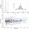 |
Fig. 1. Cluster membership for the Coma cluster with the PEAK+GAP algorithm. Top panel: redshift distribution of the objects in our spectroscopic catalog. Vertical red lines identify the redshift window with the possible member candidates, as obtained from the PEAK method. The inset displays a zoom-in of this window, with a smaller bin size for illustration purposes. Bottom panel: peculiar velocity-clustercentric distance plane from the GAP algorithm. Bona fide members are plotted with black points, while rejected candidates are shown in red. Cyan horizontal lines with squares indicate the mean peculiar velocity on each bin, while blue lines with diamonds correspond to the 3σ limit. The vertical black dotted line marks the radius up to which the gap algorithm is reliable, since the standard deviations systematically increase from this point. All the candidates outside this radius are discarded. |
Compared to the ICL fraction measured with CICLE for other clusters in previous works (Jiménez-Teja & Dupke 2016; Jiménez-Teja et al. 2018), we observe that the values estimated for Coma have larger errors. This is reasonable given that the previous analyses used imaging of exceptional quality and depth, as obtained by the Cluster Lensing and Supernovae Survey with Hubble (CLASH, Postman et al. 2012) and Frontier Fields programs (FF, Lotz et al. 2017) with the Hubble Space Telescope (HST). Moreover, the precision of CICLE depends on the geometry of the BCG+ICL system, yielding higher errors when the two components have a similar shape (profile) or luminosity (Jiménez-Teja & Dupke 2016). In the case of the Coma cluster, we found that the two BCGs and the ICL had very similar fluxes, and the signal-to-noise ratio of the images was lower than that of the HST images, thus resulting in larger errors.
As CICLE distinguishes the ICL from the BCG by determining the points where the curvature changes most strongly, the results are not biased by the PSF effect. As the PSF spreads the light of the sources, CICLE finds that the radii where the change of curvature occurs are larger for PSF-convolved sources. In this way, CICLE always calculates total fluxes, so that the estimated ICL fractions at different wavelengths can be directly compared, without the need of applying any correction. In order to confirm this statement, we calculated the PSFs of the seven J-PLUS images and created mock images with the same observational characteristics as the original BCG+ICL surface (surface brightness, effective radius, signal-to-noise ratio, etc). The test consisted of applying CICLE to the simulated images before and after convolving with each corresponding PSF. Then, the flux of the ICL estimated by CICLE was compared to the real flux of the simulated profiles. Results showed that CICLE systematically found the transition from the BCG to the ICL-dominated region at larger radii in the case of the PSF-convolved images. In relation with the unconvolved images, the error in the estimation of the ICL flux in the PSF-convolved images was larger for the J0410, J0515, and g filters, smaller for the J0430, and nearly unchanged for the J0395, r, and i bands. Thus, no correlation is observed between the estimated ICL fractions with wavelength, and no artificial bias should be introduced when the ICL fractions of different filters are compared.
5. Discussion
We analyze the implications of the results by a) comparing the ICL fractions obtained for Coma with those of the clusters studied in the previous works with HST data, and b) studying the morphology of the luminous distribution of the ICL, as in Adami et al. (2005a).
5.1. Analysis of the ICL fraction: the blue excess
Jiménez-Teja et al. (2018) analyzed a sample of 11 CLASH and FF galaxy clusters in the redshift range 0.18 < z < 0.54 whose dynamical stages were clearly stated by different indicators. Measuring their ICL fractions in three different HST optical filters (F435W, F606W, and F814W), we found that the contribution of the ICL to the total luminosity of the cluster was similar and nearly wavelength independent for the subsample of relaxed clusters (with ICL fractions varying in the interval ∼2%−11%), which would be expected if the stellar populations in the ICL and the cluster galaxies were similar and might just be equally evolving passively. However, for the subsample of merging clusters, we observed higher ICL fraction values in general in the three filters (∼7−23%), which was significantly accentuated in the case of the F606W band. Filter F606W was identified as the one mainly comprising the emission peaks of F- and A-type stars at this redshift range. Given that Morishita et al. (2017) identified a non-negligible amount of A- or earlier-type stars contributing significantly to the ICL mass budget in the FF clusters (between 5% and 10%), we suggested that the ICL fraction excess in the F606W band might be caused by these bluer stars, which might have been extracted from the outskirts of the infalling galaxies and groups to the ICL during the merging event. This excess ICL fraction observed in a particular wavelength band in merging clusters opened a “clean” window to determine the dynamical state of galaxy clusters based solely on the spectrum of the ICL fraction. If our suggested hypothesis for this effect is correct, we expect an ICL excess at about 3800 Å–4800 Å for a cluster dynamically active at redshift near zero, that is, reacting to a recent merging, and this is what our observations suggest for the Coma cluster as described below.
In Coma we find relatively high ICL fractions (between ∼7% and ∼21%, depending on the filter used), which are consistent with previous works (Melnick et al. 1977; Thuan & Kormendy 1977; Mattila 1977; Bernstein et al. 1995; Adami et al. 2005a). These might be indicative of a non-relaxed state of the cluster according to the values found for higher-redshift systems in Jiménez-Teja et al. (2018). Compared to other nearby galaxy clusters such as Fornax (Iodice et al. 2017) or Virgo (Mihos et al. 2017), Coma shows more discrepancies with the former. Fornax is believed to be a dynamically evolved, non-merging cluster, which is translated into an ICL color distribution that well represents that of its member galaxies and also a low ICL fraction (lower than 5% in the g band). Its ICL is believed to be formed from stars and globular clusters stripped out from the outskirsts of galaxies, as we suggest for the case of Coma. Virgo shows many indications of being in an unrelaxed stage, such as the substructure observed in both its spatial and kinematic distributions, or the variety of morphological types displayed by its galaxy members. Like Coma, Virgo presents some ICL tidal features that are bluer than the inner regions of its massive ellipticals, although this effect is more pronounced in the case of Coma. Although measured with a different technique, it has an estimated ICL fraction of ∼7%−15% in the V band, which is comparable to the range of ∼7%−21% spanned by Coma (albeit somewhat smaller) and consistent with the sample of merging clusters analyzed in Jiménez-Teja et al. (2018).
However, as previously described, the most characteristic feature to confirm its dynamical stage is the possible excess in the filter (or filters) to which the flux of the F- and A-type stars contributes most. At the redshift of the Coma cluster, z ∼ 0.023, if the system were in an active phase, for example, because of a recent merger, we would expect an ICL fraction peak at about 4400 Å ± ∼ 500Å. In Fig. 2 we present the ICL fraction obtained for each filter. Transmission curves of the filters are also plotted at the bottom to show how the narrow- and broadband filters overlap, so that their associated ICL fractions are not completely independent. As in Jiménez-Teja et al. (2018), we used the emission peaks of the different stellar types at the cluster redshift to split the covered wavelength range into four regions that can be compared with the transmission curves. We again identify a peak in the ICL fraction measured for the filters that mainly comprise the emission peaks of F- and A-type stars at the redshift of the Coma cluster, namely the bluer narrow filters J0395, J0410, and J0430. Although the g band also encompasses the emission peaks of the F-type stellar population, its contribution seems to be smoothed out by the width of the filter. Moreover, it should be noted that the partial overlap of the filter means that the ICL fraction excess in the blue filters measured here is a conservative lower limit estimate. Figure 2 clearly shows that the g filter overlap with the bluer narrow bands should reduce the gradient intensity.
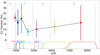 |
Fig. 2. ICL fractions for Coma as a function of the wavelength. Transmission curves of the seven J-PLUS filters we analyzed are shown, with the same color code as the ICL fractions. Vertical gray lines delimit the intervals were the emission peaks of each stellar spectral type are contained, as indicated at the top of each region. |
A simple test to estimate the significance for a change in the ICL fractions of the bluer, narrow bands J0395, J0410, and J0430 compared to those of the redder filters g, J0515, r, and i is comparing their error-weighted averages. In this way, we obtained that gradient observed in the ICL fraction is significant at 2.4σ. A more sophisticated statistical analysis is testing the null hypothesis that the ICL fraction dependence on the wavelength is flat. With this aim, we randomly generated different ICL fraction values within the error bars for each filter and applied a Kolmogorov–Smirnov test to each realization of the ICL fractions. After 106 realizations, we obtained that the null hypothesis is rejected (and thus there exists a wavelength dependence/gradient in the ICL fraction) in 99.99% of the cases with a significance of 2.6σ. This gradient is consistent with what we found for our higher redshift subsample of merging clusters in Jiménez-Teja et al. (2018).
Analyses of the population of intracluster globular cluster (IGC) in the Coma cluster core (Peng et al. 2011; Cho et al. 2016), revealed that the IGC color distribution is bimodal, with blue, metal-poor IGCs outnumbering red, metal-rich IGCs. In spite of observing a bluer ICL, they find that the fraction of red IGCs is non-negligible, representing 20% of the IGCs in the cluster core. Our study of the ICL fraction with narrow filters in the Coma cluster indeed confirms that the ICL is bluer than the galaxy members of the cluster, as in previous works (Mattila 1977; Thuan & Kormendy 1977), while at the same time, we see a significant amount of red ICL stars.
This is consistent with a scenario where part of the ICL is composed of bluer, that is, younger or lower metallicity, stars that are stripped from the outskirts of infalling galaxies or dwarfs that were disrupted during past or ongoing merging events (Peng et al. 2011; Jiménez-Teja et al. 2018). In their study of 142 early-type galaxy members of Coma (mainly drawn from the core), den Brok et al. (2011) found that almost all of them indeed had negative radial color gradients, indicating that stars in the outskirts of the galaxies are bluer than those closer to the center. This also agrees with recent integral field unit results of nearby galaxies with CALIFA (González-Delgado et al. 2015). Although den Brok et al. (2011) did not observe any dependency of the steepness of the color gradient on the radial distance to the center of the cluster (which they noted might be a selection effect), a comparison with galaxies in a lower-density environment such as Fornax revealed that the latter had much stronger metallicity gradients. Moreover, the size of the outer disks of lenticular and spiral galaxies in the center of the Coma cluster are ∼30 − 82% smaller than their counterparts in lower dense environments (e.g., Weinzirl et al. 2014 and references therein). These facts would support not only the hypothesis that these galaxies could have already lost their outer stellar layers (as has been pointed out by Thuan & Kormendy 1977), causing a bluer ICL and flattening the color gradient of Coma galaxies, but also the idea that the merging process in the core of Coma started more than a crossing time ago, and is in a very advanced (but still ongoing) stage. Assuming an average age for an A/F-type star of ∼2.3 × 10⁹ years using a Salpeter IMF from 1.1 − 2.5 M⊙, and also assuming that they were extracted halfway through their lifetimes, the presence of this ICL fraction excess would indicate that the merger probably occurred less than ∼1.2 × 10⁹ years ago.
5.2. Morphology of the ICL
In Fig. 3 we show spatial distribution of the ICL in the core of the Coma cluster for the seven J-PLUS filters we analyzed. We observe that the diffuse light is mainly spread over a common envelope containing the two giant galaxies NGC 4874 (immediately below the masked, very bright star with spikes) and NGC 4889 (east of NGC 4874). The ICL distribution is clearly elongated eastward, as reported by many authors (Kormendy & Bahcall 1974; Mattila 1977; Thuan & Kormendy 1977; Adami et al. 2005a). This lack of symmetry again confirms that Coma is far from being relaxed. For wavelengths redder than the J0430 band, we see a clear arc-shaped extension of diffuse light spreading to the southwest from NGC 4874 (as in Welch & Sastry 1971; Kormendy & Bahcall 1974; Mattila 1977; Melnick et al. 1977), which is associated with a change in the ICL position angle, from ∼80° in the narrow blue filters to ∼55 − 65° in redder bands. This implies that the red stars in the ICL closely follow the overall distribution of the galaxy members, since the cluster major axis is estimated to be at a position angle of 64–65° (Rood et al. 1972; Thuan & Kormendy 1977).
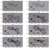 |
Fig. 3. Contour maps of the ICL in the central region of the Coma clusters superimposed on the original data, and guiding image to identify the ICL substructure (bottom right panel). Original images have the stars and spikes masked out. We have smoothed the surface distribution of the ICL with a Gaussian of 17.6 arcsec typical deviation to draw the contours. Masked-out pixels were not considered to estimate the ICL fraction or calculate the contours. The guiding image at the bottom right shows the original image in the i band with the main galaxies (blue stars) and ICL clumps (red letters) labeled. North is up and east is to the left. |
Previous works have reported that the ICL southeast edge is very sharp (especially south of NGC 4889) compared to the northwest bridge, whose intensity drops smoothly (Kormendy & Bahcall 1974; Melnick et al. 1977). In addition to its morphology, the dynamical activity in Coma is reflected in the paucity of smoothness and homogeneity of the ICL, where we can observe substructures. The bottom right panel in Fig. 3 shows that the diffuse light is mainly concentrated around NGC 4874 (clump A) at every wavelength (consistently with the distribution found by Adami et al. 2005a), although we cannot be sure that the ICL emission peak and the centroid of the giant elliptical are completely aligned because of the proximity of the bright star that might be altering the isocontours. We do see the absence of an emission peak centered on NGC 4889. Instead, the diffuse light is preferentially concentrated on two clumps, east and west of this giant galaxy, which are evident in all the filters, but most intensely in the bluer narrow bands (marked in Fig. 3 as B and C). Although slightly displaced with respect to our measurements, the existence of an ICL clump in between the two D galaxies (B) has been noted by Adami et al. (2005a; as well as several other substructures north of NGC 4874 that we are unable to confirm because they lie above our masked area). Given that strong tidal forces are expected to occur between the two giant galaxies, it is not surprising that this region (B) is observed to be ICL rich. Stripping of the stars in the outskirts of the massive galaxies and the total disruption of dwarfs would be more efficient mechanisms in this region.
To our knowledge, clump C, east of NGC 4889, has not been reported before. Based on a comparison of its location with the likely orbits of the two dominant galaxies during the merger (Fig. 2 of Gerhard et al. 2007), we suggest that it might have been formed from the surroundings of NGC 4874 and its associated group during its travel to the bottom of the potential well. A dynamical study of the velocity distribution of planetary nebulae in this region could verify the association with NGC 4874 and test this scenario.
In addition to these three main clumps of ICL closer to the center of Coma, we observed at least three other different structures in Fig. 3: the reddish arc-shaped ridge spreading southwest of NGC 4874 (D); the more subtle, elongated extension of light east of NGC 4889 (E); and the two very blue clumps associated with the spiral galaxies NGC 4921 and NGC 4911, southeast of NGC 4889 (F and G respectively).
The D and E substructures have previously been observed by other authors (Welch & Sastry 1971; Kormendy & Bahcall 1974; Melnick et al. 1977; Thuan & Kormendy 1977). They are very irregular according to their isocontours: multiple small peaks of ICL are distributed throughout these regions, apparently without a dominant clump. The slope of the diffuse light distribution is fainter in both areas than the distribution in the A, B, and C clumps of the cluster core. A significant difference is that the SW extension D (ridge) does not appear in the bluest filters, while the E substructure is visible in all bands. The lack of bluer ICL in D may suggest that this is an earlier region affected by the merger, where most of the stripped A- and F-type stars are already dead. The morphological density contour maps calculated by Adami et al. (2008) reveal density clumps in the E region for all morphological types, although strongly dominated by early type galaxies. With a bit less intensity, the D substructure is also primarily dominated by early type galaxies, although it shows a non-negligible contribution from irregulars too. However, these density maps show a clear deficit of spirals and starbursts in this region, which would explain its lack of luminosity in the bluest filters.
Early works on the ICL of Coma have reported the clumps F and G (e.g., Melnick et al. 1977). Neither of them seems to be connected to the main envelope of ICL surrounding the giant ellipticals of the center, at least down to our detection limit. In the J0430 band alone, clump G appears weakly connected to the main ICL structure, but with low significance. Both clumps are very blue, whereas they appear much weaker in the red bands, which is expected because these regions show a higher density of irregular and starbust galaxies than the surroundings (Adami et al. 2008). In particular, the F clump is as blue as the two main concentrations of ICL in the core (A and B). According to Adami et al. (2005b), the two spirals NGC 4921 and NGC 4911 belong to two dynamically independent groups that could be falling into the cluster following tangential orbits. This agrees with the fact that clumps F and G show no significant indication of being linked at any wavelength, according to our ICL contour maps.
6. Conclusions
Jiménez-Teja et al. (2018) showed that the ICL fraction distribution across different wavelengths could be used as an estimator of the dynamical state of massive systems using HST data of a sample of galaxy clusters distributed in the redshift range 0.18 < z < 0.54. Our new analysis of the ICL fraction of Coma not only confirms that it is a dynamically active system, but also that the ICL fraction can be an indicator of the dynamic stage for nearby clusters when the filters are selected appropriately. The J-PLUS filter system has been proved to be an appropriate set for studying the ICL fraction distribution across wavelengths in nearby clusters, given its combination of narrow- and broadband filters. We must remark that using the traditional SDSS filter system alone, we might not significantly detect the ICL fraction excess, which is characteristic of dynamical activity.
With Coma as a case study, we have also tested the capabilities and the quality of the J-PLUS data for analyzing the diffuse light in galaxy clusters in terms of depth and precision. Despite the larger errors that are due to the special geometry of the Coma BCG+ICL system and the lower signal-to-noise ratio of the J-PLUS images (compared to that of the HST observations), we proved that we can obtain reliable measurements of the ICL fraction with CICLE applied to J-PLUS data. Estimated ICL fractions range from ∼7% to ∼21%, consistent with previous values reported in the literature for similar wavelengths (usually green and red filters). We also extended the traditional study of the diffuse light in Coma to bluer bands, revealing the characteristic excess in the ICL fraction measured in the filters which comprises the emission peaks of F- and A-type stars, and is typical of merging clusters (Jiménez-Teja et al. 2018).
We also took advantage of the multicolor J-PLUS system to analyze the varying morphology of the ICL at different wavelengths (see Fig. 3). The complex, elongated, asymmetric, and clumpy structure of the ICL confirms that Coma is far from a virialized state. CICLE results confirmed several features that have previously been reported in the literature, such as the main concentration around the NGC 4874 (A), the clump in between the two BCGs (B), the elongated eastward extension (E), the reddish arc-shaped feature southwest of NGC 4874 (D), and the blue concentrations associated with the spirals NGC 4921 and NGC 4911 (F and G; e.g., Melnick et al. 1977; Thuan & Kormendy 1977; Adami et al. 2005a). We also found a new feature: a multicolored peak east of NGC 4889 (C), visible throughout our entire wavelength range. The distribution and colors of all these features represent independent evidence that confirms the dynamical scenario proposed by several authors in previous works for the Coma cluster (e.g., Colless & Dunn 1996; Adami et al. 2005b; Gerhard et al. 2007).
Although the obtained results are consistent with those found in the literature, in the future we aim to complement our study with new J-PLUS observations. Images with a higher signal-to-noise ratio and the study of the filters that were not included in this work, either because they were not observed or because the images presented some kind of artifact, will be essential to reduce the errors of the estimated ICL fractions and increase the significance of the ICL fraction excess. A study of the stellar populations in different regions of the ICL of Coma will be described in a future paper, using the J-PLUS photometry as low-resolution spectra.
Acknowledgments
We gratefully acknowledge the computational support of Fernando Roig. Y. J-T. also acknowledges financial support from the Fundação Carlos Chagas Filho de Amparo à Pesquisa do Estado do Rio de Janeiro – FAPERJ (fellowship Nota 10, PDR-10) through grant E-26/202.835/2016. R.A.D. acknowledges support from the Conselho Nacional de Desenvolvimento Científico e Tecnológico – CNPq through BP grant 312307/2015-2, and the Financiadora de Estudos e Projetos – FINEP grants REF. 1217/13 – 01.13.0279.00 and REF 0859/10 – 01.10.0663.00 for hardware support for the J-PLUS project through the National Observatory of Brazil and CBPF. Both Y. J-T. and R.A.D. also acknowledge support from the Spanish National Research Council – CSIC (I-COOP+ 2016 program) through grant COOPB20263, and the Spanish Ministry of Economy, Industry, and Competitiveness – MINECO through grants AYA2013-48623-C2-1-P and AYA2016-81065-C2-1-P. R.L.O. was partially supported by the Brazilian agency CNPq (PDE 200289/2017-9, Universal Grants 459553/2014-3, PQ 302037/2015-2). J. A. H. J. thanks the Brazilian institution CNPq for financial support through a postdoctoral fellowship (project 150237/2017-0). Funding for the J-PLUS Project has been provided by the Governments of Spain and Aragon through the Fondo de Inversiones de Teruel, the Spanish Ministry of Economy and Competitiveness (MINECO; under grants AYA2015-66211-C2-1-P, AYA2015-66211-C2-2, AYA2012-30789, and ICTS-2009-14), and European FEDER funding (FCDD10-4E-867, FCDD13-4E-2685). We thank the OAJ Data Processing and Archiving Unit (UPAD) for reducing and calibrating the OAJ data used in this work. This research has made use of the VizieR catalogue access tool, CDS, Strasbourg, France. Funding for the Sloan Digital Sky Survey IV has been provided by the Alfred P. Sloan Foundation, the U.S. Department of Energy Office of Science, and the Participating Institutions. SDSS-IV acknowledges support and resources from the Center for High-Performance Computing at the University of Utah. The SDSS web site is www.sdss.org. SDSS-IV is managed by the Astrophysical Research Consortium for the Participating Institutions of the SDSS Collaboration including the Brazilian Participation Group, the Carnegie Institution for Science, Carnegie Mellon University, the Chilean Participation Group, the French Participation Group, Harvard-Smithsonian Center for Astrophysics, Instituto de Astrofísica de Canarias, The Johns Hopkins University, Kavli Institute for the Physics and Mathematics of the Universe (IPMU)/University of Tokyo, Lawrence Berkeley National Laboratory, Leibniz Institut für Astrophysik Potsdam (AIP), Max-Planck-Institut für Astronomie (MPIA Heidelberg), Max-Planck-Institut für Astrophysik (MPA Garching), Max-Planck-Institut für Extraterrestrische Physik (MPE), National Astronomical Observatories of China, New Mexico State University, New York University, University of Notre Dame,Observatário Nacional/MCTI, The Ohio State University, Pennsylvania State University, Shanghai Astronomical Observatory, United Kingdom Participation Group,Universidad Nacional Autónoma de México,University of Arizona, University of Colorado Boulder, University of Oxford, University of Portsmouth, University of Utah, University of Virginia, University of Washington, University of Wisconsin, Vanderbilt University, and Yale University.
References
- Albareti, F. D., Allende Prieto, C., Almeida, A., et al. 2017, ApJS, 233, 25 [NASA ADS] [CrossRef] [Google Scholar]
- Adami, C., Slezak, E., Durret, F., et al. 2005a, A&A, 429, 39 [NASA ADS] [CrossRef] [EDP Sciences] [Google Scholar]
- Adami, C., Biviano, A., Durret, F., & Mazure, A. 2005b, A&A, 443, 17 [NASA ADS] [CrossRef] [EDP Sciences] [Google Scholar]
- Adami, C., Ilbert, O., Pelló, R., et al. 2008, A&A, 491, 681 [NASA ADS] [CrossRef] [EDP Sciences] [Google Scholar]
- Arnaud, M., Aghanim, N., Gastaud, R., et al. 2001, A&A, 365, L67 [NASA ADS] [CrossRef] [EDP Sciences] [Google Scholar]
- Benítez, N., Dupke, R., Moles, M., et al. 2014, ArXiv e-prints [arXiv:1403.5237] [Google Scholar]
- Beijersbergen, M., Hoekstra, H., van Dokkum, P. G., & van der Hulst, T. 2002, MNRAS, 329, 385 [NASA ADS] [CrossRef] [Google Scholar]
- Bernstein, G. M., Nichol, R. C., Tyson, J. A., Ulmer, M. P., & Wittman, D. 1995, AJ, 110, 1507 [NASA ADS] [CrossRef] [Google Scholar]
- Bertin, E. 2006, in Astronomical Data Analysis Software and Systems XV, eds. C. Gabriel, C. Arviset, D. Ponz, & S. Enrique, ASP Conf. Ser., 351, 211 [Google Scholar]
- Bertin, E. 2011, in ASP Conf. Ser., eds. I. N. Evans, A. Accomazzi, D. J. Mink, & A. H. Rots, 442, 435 [Google Scholar]
- Bertin, E., & Arnouts, S. 1996, A&AS, 117, 393 [NASA ADS] [CrossRef] [EDP Sciences] [Google Scholar]
- Bertin, E., Mellier, Y., Radovich, M., et al. 2002, in Astronomical Data Analysis Software and Systems XI, eds. D. A. Bohlender, D. Durand, &T. H. Handley, ASP Conf. Ser., 281, 228 [NASA ADS] [Google Scholar]
- Blanton, M. R., Bershady, M. A., Abolfathi, B., et al. 2017, AJ, 154, 28 [NASA ADS] [CrossRef] [Google Scholar]
- Boschin, W., Girardi, M., Spolaor, M., & Barrena, R. 2006, A&A, 449, 461 [NASA ADS] [CrossRef] [EDP Sciences] [Google Scholar]
- Briel, U. G., Henry, J. P., & Böhringer, H. 1992, A&A, 259, L31 [NASA ADS] [Google Scholar]
- Briel, U. G., Henry, J. P., Lumb, D. H., et al. 2011, A&A, 365, L60 [NASA ADS] [CrossRef] [EDP Sciences] [Google Scholar]
- Brown, S., & Rudnick, L. 2011, MNRAS, 412, 2 [NASA ADS] [CrossRef] [Google Scholar]
- Burke, C., Collins, C. A., Stott, J. P., & Hilton, M. 2012, MNRAS, 425,2058 [Google Scholar]
- Cenarro, A. J., Moles, M., Cristóbal-Hornillos, D., et al. 2019, A&A, 622, A176 [Google Scholar]
- Cho, H., Blakeslee, J. P., Chies-Santos, A. L., et al. 2016, ApJ, 822, 95 [NASA ADS] [CrossRef] [Google Scholar]
- Colless, M., & Dunn, A. M. 1996, ApJ, 458, 435 [NASA ADS] [CrossRef] [Google Scholar]
- Conselice, C. J., & Gallagher, III, J. S. 1998, MNRAS, 297, L34 [NASA ADS] [CrossRef] [Google Scholar]
- Cristóbal-Hornillos, D., Gruel, N., Varela, J., et al. 2012, Software and Cyberinfrastructure for Astronomy II, Proc. SPIE, 8451, 845116 [CrossRef] [Google Scholar]
- Davis, S. D., & Mushotzky, R. F. 1993, AJ, 105, 409 [NASA ADS] [CrossRef] [Google Scholar]
- Deiss, B. M., Reich, W., Lesch, H., & Wielebinski, R. 1997, A&A, 321, 55 [NASA ADS] [Google Scholar]
- den Brok, M., Peletier, R. F., Valentijn, E. A., et al. 2011, MNRAS, 414, 3052 [Google Scholar]
- de Vaucouleurs, G., & de Vaucouleurs, A. 1970, Astrophys. Lett., 5, 219 [NASA ADS] [Google Scholar]
- Edge, A. C., Stewart, G. C., & Fabian, A. C. 1992, MNRAS, 258, 177 [NASA ADS] [CrossRef] [Google Scholar]
- Fadda, D., Girardi, M., Giuricin, G., Mardirossian, F., & Mezzetti, M. 1996, ApJ, 473, 670 [NASA ADS] [CrossRef] [Google Scholar]
- Fitchett, M., & Webster, R. 1987, ApJ, 317, 653 [NASA ADS] [CrossRef] [Google Scholar]
- Gavazzi, G., Savorgnan, G., & Fumagalli, M. 2011, A&A, 534, A31 [NASA ADS] [CrossRef] [EDP Sciences] [Google Scholar]
- Gerhard, O., Arnaboldi, M., Freeman, K. C., et al. 2007, A&A, 468, 815 [NASA ADS] [CrossRef] [EDP Sciences] [Google Scholar]
- Giovannini, G., Feretti, L., & Andernach, H. 1985, A&A, 150, 302 [NASA ADS] [Google Scholar]
- Girardi, M., Fadda, D., Giuricin, G., Mardirossian, F., & Mezzetti, M. 1996, ApJ, 457, 61 [NASA ADS] [CrossRef] [Google Scholar]
- González-Delgado, R. M., García-Benito, R., Péres, E., et al. 2015, A&A, 581, A103 [NASA ADS] [CrossRef] [EDP Sciences] [Google Scholar]
- Gregg, M. D., & West, M. J. 1998, Nature, 396, 549 [NASA ADS] [CrossRef] [Google Scholar]
- Gunn, J. E. 1969, BAAS, 1, 191 [NASA ADS] [Google Scholar]
- Iodice, E., Spavone, M., Cantiello, M., et al. 2017, ApJ, 851, 75 [Google Scholar]
- Jafe, W. J., Perola, G. C., & Valentijn, E. A. 1976, A&A, 49, 179 [NASA ADS] [Google Scholar]
- Jiménez-Teja, Y., & Benítez, N. 2012, ApJ, 745, 150 [NASA ADS] [CrossRef] [Google Scholar]
- Jiménez-Teja, Y., & Dupke, R. 2016, ApJ, 820, 49 [NASA ADS] [CrossRef] [Google Scholar]
- Jiménez-Teja, Y., Dupke, R., Benítez, N., et al. 2018, ApJ, 857, 79 [NASA ADS] [CrossRef] [Google Scholar]
- Johnson, M. W., Cruddace, R. G., Fritz, G., Shulman, S., & Friedman, H. 1979, ApJ, 231, L45 [NASA ADS] [CrossRef] [Google Scholar]
- Kent, S. M., & Gunn, J. E. 1982, AJ, 87, 945 [NASA ADS] [CrossRef] [Google Scholar]
- Kim, K.-T., Kronberg, P. P., Dewdney, P. E., & Landecker, T. L. 1990, ApJ, 355, 29 [NASA ADS] [CrossRef] [Google Scholar]
- Kormendy, J., & Bahcall, J. N. 1974, AJ, 79, 671 [NASA ADS] [CrossRef] [Google Scholar]
- Krick, J. E., & Bernstein, R. A. 2007, AJ, 134, 466 [Google Scholar]
- Kronberg, P. P., Kothes, R., Salter, C. J., & Perillat, P. 2007, ApJ, 659, 267 [NASA ADS] [CrossRef] [Google Scholar]
- Kubo, J. M., Stebbins, A., Annis, J., et al. 2007, ApJ, 671, 1466 [NASA ADS] [CrossRef] [Google Scholar]
- Lotz, J. M., Koekemoer, A., Coe, D., et al. 2017, ApJ, 837, 97 [Google Scholar]
- Mahajan, S., Haines, C. P., & Raychaudhury, S. 2010, MNRAS, 404, 1745 [NASA ADS] [Google Scholar]
- Mattila, K. 1977, A&A, 60, 425 [NASA ADS] [Google Scholar]
- Mellier, Y., Mathez, G., Mazure, A., Chauvineau, B., & Proust, D. 1988, A&A, 199, 67 [NASA ADS] [Google Scholar]
- Melnick, J., White, S. D. M., & Hoessel, J. 1977, MNRAS, 180, 207 [NASA ADS] [CrossRef] [Google Scholar]
- Mendelin, M., & Binggeli, B. 2017, A&A, 604, A96 [NASA ADS] [CrossRef] [EDP Sciences] [Google Scholar]
- Merritt, D. 1987, ApJ, 313, 121 [NASA ADS] [CrossRef] [Google Scholar]
- Merritt, D., & Tremblay, B. 1994, AJ, 108, 514 [NASA ADS] [CrossRef] [Google Scholar]
- Mihos, J. C., Harding, P., Feldmeier, J. J., et al. 2017, ApJ, 834, 16 [NASA ADS] [CrossRef] [Google Scholar]
- Morishita, T., Abramson, L. E., Treu, T., et al. 2017, ApJ, 846, 139 [NASA ADS] [CrossRef] [Google Scholar]
- Neumann, D. M., Arnaud, M., Gastaud, R., et al. 2001, A&A, 365, L74 [NASA ADS] [CrossRef] [EDP Sciences] [Google Scholar]
- Neumann, D. M., Lumb, D. H., Pratt, G. W., & Briel, U. G. 2003, A&A, 400, 811 [NASA ADS] [CrossRef] [EDP Sciences] [Google Scholar]
- Owers, M. S., Randall, S. W., Nulsen, P. E. J., et al. 2011, ApJ, 728, 27 [NASA ADS] [CrossRef] [Google Scholar]
- Patrikalakis, N. M., & Maekawa, T. 2002, Shape Interrogation for Computer Aided Design and Manufacturing (Berlin: Springer) [Google Scholar]
- Peng, E. W., Ferguson, H. C., Goudfrooij, P., et al. 2011, ApJ, 730, 23 [NASA ADS] [CrossRef] [Google Scholar]
- Postman, M., Coe, D., Benítez, N., et al. 2012, ApJS, 199, 25 [NASA ADS] [CrossRef] [Google Scholar]
- Rood, H. J., Page, T. L., Kintner, E. C., & King, I. R. 1972, ApJ, 175, 627 [NASA ADS] [CrossRef] [Google Scholar]
- Simionescu, A., Werner, N., Urban, O., et al. 2013, ApJ, 775, 4 [NASA ADS] [CrossRef] [Google Scholar]
- Smith, R. J., Lucey, J. R., Hudson, M. J., et al. 2009, MNRAS, 392, 1265 [NASA ADS] [CrossRef] [Google Scholar]
- Strauss, M. A., Weinberg, D. H., Lupton, R. H., et al. 2002, ApJ, 124, 1810 [Google Scholar]
- Thuan, T. X., & Kormendy, J. 1977, PASP, 89, 466 [NASA ADS] [CrossRef] [Google Scholar]
- Trentham, N., & Mobasher, B. 1998, MNRAS, 293, 53 [NASA ADS] [CrossRef] [Google Scholar]
- Ulmer, M. P., Nichol, R. C., & Martin, D. R. 1994, in Proceedings of an ESO/OHP Workshop on Dwarf Galaxies, eds. G. Meylan, & P. Prugniel, 121 [Google Scholar]
- van Dokkum, P. G. 2001, PASP, 113, 1420 [NASA ADS] [CrossRef] [Google Scholar]
- Venturi, T., Giovannini, G., & Feretti, L. 1990, AJ, 99, 1381 [NASA ADS] [CrossRef] [Google Scholar]
- Vikhlinin, A., Forman, W., & Jones, C. 1997, ApJ, 474, L7 [NASA ADS] [CrossRef] [Google Scholar]
- Watt, M. P., Ponman, T. J., Bertram, D., et al. 1992, MNRAS, 258, 738 [NASA ADS] [CrossRef] [Google Scholar]
- Weinzirl, T., Jogee, S., Neistein, E., et al. 2014, MNRAS, 441, 3083 [NASA ADS] [CrossRef] [Google Scholar]
- Welch, G. A., & Sastry, G. N. 1971, ApJ, 169, L3 [NASA ADS] [CrossRef] [Google Scholar]
- White, S. D. M., Briel, U. G., & Henry, J. P. 1993, MNRAS, 261, L8 [NASA ADS] [CrossRef] [Google Scholar]
- Willson, M. A. G. 1970, MNRAS, 151, 1 [NASA ADS] [CrossRef] [Google Scholar]
- Zemcov, M., Immel, P., Nguyen, C., et al. 2017, Nat. Commun., 8, 15003 [NASA ADS] [CrossRef] [Google Scholar]
- Zwicky, F. 1957, Morphological Astronomy (Berlin: Springel-Verlag) [CrossRef] [Google Scholar]
All Tables
All Figures
|
Fig. 1. Cluster membership for the Coma cluster with the PEAK+GAP algorithm. Top panel: redshift distribution of the objects in our spectroscopic catalog. Vertical red lines identify the redshift window with the possible member candidates, as obtained from the PEAK method. The inset displays a zoom-in of this window, with a smaller bin size for illustration purposes. Bottom panel: peculiar velocity-clustercentric distance plane from the GAP algorithm. Bona fide members are plotted with black points, while rejected candidates are shown in red. Cyan horizontal lines with squares indicate the mean peculiar velocity on each bin, while blue lines with diamonds correspond to the 3σ limit. The vertical black dotted line marks the radius up to which the gap algorithm is reliable, since the standard deviations systematically increase from this point. All the candidates outside this radius are discarded. |
| In the text | |
|
Fig. 2. ICL fractions for Coma as a function of the wavelength. Transmission curves of the seven J-PLUS filters we analyzed are shown, with the same color code as the ICL fractions. Vertical gray lines delimit the intervals were the emission peaks of each stellar spectral type are contained, as indicated at the top of each region. |
| In the text | |
|
Fig. 3. Contour maps of the ICL in the central region of the Coma clusters superimposed on the original data, and guiding image to identify the ICL substructure (bottom right panel). Original images have the stars and spikes masked out. We have smoothed the surface distribution of the ICL with a Gaussian of 17.6 arcsec typical deviation to draw the contours. Masked-out pixels were not considered to estimate the ICL fraction or calculate the contours. The guiding image at the bottom right shows the original image in the i band with the main galaxies (blue stars) and ICL clumps (red letters) labeled. North is up and east is to the left. |
| In the text | |
Current usage metrics show cumulative count of Article Views (full-text article views including HTML views, PDF and ePub downloads, according to the available data) and Abstracts Views on Vision4Press platform.
Data correspond to usage on the plateform after 2015. The current usage metrics is available 48-96 hours after online publication and is updated daily on week days.
Initial download of the metrics may take a while.