| Issue |
A&A
Volume 666, October 2022
|
|
|---|---|---|
| Article Number | A54 | |
| Number of page(s) | 12 | |
| Section | Extragalactic astronomy | |
| DOI | https://doi.org/10.1051/0004-6361/202243504 | |
| Published online | 04 October 2022 | |
Physical properties of more than one thousand brightest cluster galaxies detected in the Canada-France-Hawaii Telescope Legacy Survey
1
Sorbonne Université, CNRS, UMR 7095, Institut d’Astrophysique de Paris, 98bis Bd Arago, 75014 Paris, France
e-mail: aline.chu@iap.fr
2
Jodrell Bank Centre for Astrophysics, University of Manchester, Oxford Road, Manchester, UK
3
IRAP, Institut de Recherche en Astrophysique et Planétologie, Université de Toulouse, UPS-OMP, CNRS, CNES, 14 avenue E. Belin, 31400 Toulouse, France
4
Instituto de Astrofísica de Andalucía, CSIC, Glorieta de la Astronomía s/n, 18008 Granada, Spain
Received:
9
March
2022
Accepted:
28
June
2022
Context. Brightest cluster galaxies (BCGs) are very massive elliptical galaxies found at the centres of clusters. Their study gives clues to the formation and evolution of the clusters in which they are embedded.
Aims. We analyse here in a homogeneous way the properties of a sample of more than 1000 BCGs in the redshift range 0.15 < z < 0.7, based on images from the Canada-France-Hawaii Telescope Legacy Survey.
Methods. Based on a recent catalogue of 1371 clusters, we applied our automatic BCG detection algorithm and successfully identified 70% of the BCGs in our sample. We analysed their 2D photometric properties with GALFIT. We also compared the position angles of the BCG major axes with those of the overall cluster to which they belong.
Results. We find no evolution of the BCG properties with redshift up to z = 0.7, in agreement with previous results by Chu et al. (2021, A&A, 649, A42), who analysed a sample an order of magnitude smaller, but reaching a redshift z = 1.8. The Kormendy relation for BCGs is tight and consistent with that of normal elliptical galaxies and BCGs measured by other authors. The position angles of the BCGs and of the cluster to which they belong agree within 30 degrees for 55% of the objects with well-defined position angles.
Conclusions. The study of this very large sample of more than 1000 BCGs shows that they were mainly formed before z = 0.7 as we find no significant growth for the luminosities and sizes of central galaxies. We discuss the importance of the intracluster light in the interpretation of these results. We highlight the role of image depth in the modelling of the luminosity profiles of BCGs, and give evidence of the presence of an inner structure which can only be resolved on deep surveys with limiting apparent magnitude at 80% completeness m80 > 26 mag arcsec−2.
Key words: galaxies: clusters: general / galaxies: evolution / galaxies: formation
© A. Chu et al. 2022
 Open Access article, published by EDP Sciences, under the terms of the Creative Commons Attribution License (https://creativecommons.org/licenses/by/4.0), which permits unrestricted use, distribution, and reproduction in any medium, provided the original work is properly cited.
This article is published in open access under the Subscribe-to-Open model. Subscribe to A&A to support open access publication.
1. Introduction
Located at the intersection of cosmic filaments in the large-scale structures, galaxy clusters present in their centres, at the bottom of the cluster potential well, a supermassive galaxy that is also most often the brightest galaxy in the cluster. This galaxy is referred to as the brightest cluster galaxy (BCG).
It is commonly believed that BCGs are supermassive elliptical galaxies with quenched star formation and little to no gas left. Their gas was consumed during mergers that formed stars at earlier epochs, as predicted by Thomas et al. (2010), among others, who find that most of the stellar population present in such galaxies was already formed in situ before the cluster was formed at z ≃ 2. However, BCGs with huge reservoirs of molecular gas and strong ongoing star formation have been observed and identified (see McDonald et al. 2016; Fogarty et al. 2019; Castignani et al. 2020). Some of these particular BCGs also have irregular shapes instead of the regular elliptical morphology expected. Sometimes, they can even be reminiscent of jellyfish galaxies, such as RX J1532+3020 that shows traces of a recent merger, with UV-emitting filaments and knots indicating recent starbursts (Castignani et al. 2020). Such cases remain rare, as shown by Chu et al. (2021), who reported that only two BCGs out of 98 were blue galaxies (negative rest frame blue minus red colour) with a high star formation rate (SFR > 100 M⊙ yr−1). Cerulo et al. (2019) found that only 9% of the BCGs that constitute their sample of 74275 BCGs up to z = 0.35 have colours bluer than 2σ from the median colour of the red sequence.
Brightest cluster galaxies can form via numerous dynamical and environmental processes, such as galactic cannibalism, cooling flows from the central AGN, or dynamical friction, but the relative importances of these processes on the growth of BCGs and on the stellar mass assembly are still controversial (see Castignani et al. 2020, and references therein). In addition, it is unclear whether BCGs are still evolving today, as authors have found conflicting results.
Observations show that at low and intermediate redshifts (z < 1), or even at local redshifts, some BCGs can still be undergoing major mergers that could potentially affect the growth of the central galaxy. This agrees with Bernardi (2009) and Ascaso et al. (2010), for example, who find that the sizes of BCGs have grown by a factor of 2 since z = 0.5.
The galaxies that compose the cluster and constitute the red sequence of the cluster, including the BCG, are mostly red elliptical galaxies with little gas content. Major mergers were shown to have little effect on the mass growth of BCGs and to be unlikely to trigger a new starburst phase (De Lucia & Blaizot 2007). De Lucia & Blaizot (2007) show in simulations that half of the final mass of BCGs is already in place by redshift 0.5. Thomas et al. (2010) find that most of the stars in BCGs were already formed before z = 2, and De Lucia & Blaizot (2007) show that at least 80% were already formed by z = 3. These studies indicate that it is likely that the stellar population in these galaxies has settled earlier than 10 Gyr ago at least. This is consistent with Stott et al. (2011) who find no significant change in the size or shape of these galaxies since z = 1.3. Additionally, Chu et al. (2021) find that the physical properties of BCGs, such as effective radius and surface brightness, show little to no evolution since redshift z = 1.8, and conclude that BCGs were thus mainly formed before z = 1.8. BCGs undergoing major mergers (12 clusters) were also detected in this last study, and were found to have properties that did not differ from those of other BCGs.
Understanding how BCGs were formed and how they evolve can help us to understand how the clusters that host them were formed (see e.g., Lauer et al. 2014). BCGs are the result of billions of years of successive galaxy mergers that can leave an imprint on the galaxy. Numerous studies have shown that clusters are preferentially aligned in the cosmic web, along the filaments that connect them, and that neighbouring clusters separated by less than 30 Mpc tend to ‘point to each other’ (see Binggeli 1982). BCGs were also found to share this same tendency with their host clusters; Donahue et al. (2015), West et al. (2017), Durret et al. (2019), De Propris et al. (2020) and Chu et al. (2021) have found that BCGs tend to align with the major axis of the host cluster. This means that BCGs tend to have a preferential orientation pointing to the filaments of the cosmic web along which galaxies and groups are falling towards the bottom of the cluster potential well where the BCG is expected to reside. BCGs are aligned by tidal interaction (Faltenbacher et al. 2009) and show stronger alignments for brighter galaxies, for rich and more massive clusters, and for low redshifts (see Faltenbacher et al. 2009; Niederste-Ostholt et al. 2010; Hao et al. 2011). Niederste-Ostholt et al. (2010) find that the second to fifth ranked galaxies of the cluster also tend to show signs of alignment, although not as strongly as the BCG. West et al. (2017) show that other galaxies in the cluster, excluding the BCG, have no preferential orientations in the cluster.
The present study uses data from the Canada-France-Hawaii Telescope Legacy Survey (CFHTLS) and concentrates on the redshift range between 0.15 and 0.7. Although the resolution is not as good as that of the Hubble Space Telescope (HST), we increased the sample size by almost a factor of 20 (there are 74 BCGs in the same redshift range in Chu et al. 2021), making this analysis one of the largest studies on BCGs, thus allowing us to go deep into the study of the luminosity profiles of these galaxies.
The intracluster light (ICL) is also brought up in this study. The ICL is composed of stars that were stripped from their host galaxies and are now trapped in the potential of the cluster, but are not gravitationally bound to any individual galaxy in the cluster. This ICL constitutes a very diffuse and faint component of the cluster, which is thus very difficult to detect and can merge with the extended envelope of the central galaxy. One challenge is to distinguish the BCG from the ICL. Some works have shown, by studying the velocity dispersion as a function of the distance to the BCG centre, an increase in the dispersion observed at longer distances (Cui et al. 2014; Jiménez-Teja et al. 2021). This discrepancy shows the border between ICL and BCG. However, spectroscopic observations are currently necessary to achieve this. In the absence of such spectroscopic data, algorithms that attempt to detect the ICL on deep large-scale images are being developed and should allow us to detect low surface brightness objects even more efficiently on optical images in the near future. This topic is bound to become all the more important with the release of deep sky surveys (see e.g., Jiménez-Teja & Dupke 2016; Kluge et al. 2020, 2021; Ellien et al. 2021). In this paper we also discuss and estimate how much the ICL may impact the luminosity profiles of BCGs at these redshifts.
The paper is organized as follows. The data and the method used to detect the BCGs are presented in Sect. 2. In Sect. 3 we describe how the luminosity profiles were modelled, and analyse the results obtained. In Sect. 4 we estimate in a preliminary study the impact of the ICL on the models fitted, and in Sect. 5 the impact of the depth of the images. We measure the alignment of BCGs with their host clusters in Sect. 6. Finally, we discuss the results and present our conclusions in Sect. 7.
Throughout this paper we assume a ΛCDM model with H0 = 70 km s−1 Mpc−1, ΩM = 0.3, and ΩΛ = 0.7. We compute the scales and physical distances using the astropy.coordinates package1. All magnitudes are given in the AB system.
2. Obtaining the BCG catalogue
2.1. The data
This work is based on the cluster catalogue of 1371 clusters by Sarron et al. (2018), extracted in the 154 deg2 region covered by the CFHTLS with the AMASCFI cluster finder. The survey is 80% complete in AB up to a magnitude mi = 24.8 in the CFHTLS i filter, for point sources. The code detects clusters as galaxy overdensities in overlapping photometric redshift slices. Multiple detections that occur in such a configuration are then cleaned using a minimal spanning tree (MST) algorithm. The cluster candidates have a mass M200 > 1014 M⊙ and are limited to redshift z ≤ 0.7. By running the AMASCFI cluster finder on mock data created using lightcones from the Millennium simulations (Springel et al. 2005; Henriques et al. 2012) and modified to mimic CFHTLS data, Sarron et al. (2018) estimated that this cluster sample is 90% pure and 70% complete overall. At z ≤ 0.7, they find that the purity is fairly constant with redshift ∼90%, while the completeness steadily decreases with increasing redshift and decreasing cluster mass from ∼100% down to ∼50% at z ∼ 0.6 and M200 ∼ 1014 M⊙. The large number of clusters in this catalogue, with known selection function, allowed Sarron et al. (2018) to discuss the properties and evolution of cluster galaxies with redshift in various mass bins.
Photometric redshifts are available for each galaxy in the field in the CFHTLS TERAPIX T0007 release. These photo-zs were computed with the LePhare code (Arnouts et al. 1999; Ilbert et al. 2006) based on five filters in the optical.
For the purpose of this work we used the redshift probability distribution function (PDF) for each cluster, PDFc(z), computed by Adami et al. (2020) on the Sarron et al. (2018) catalogue. We note however, that contrary to Adami et al. (2020), we did not split PDFc(z) with multiple peaks into sub-detections. We made this choice in order to stay as close as possible to the original catalogue released in Sarron et al. (2018). Briefly, the cluster redshift PDF is computed by summing (stacking) the PDFgal(z) of galaxies (provided for each galaxy in the photometric redshift release of the CFHTLS T0007) less than 0.5 Mpc from the cluster centre and removing the expected field stacked PDFfield(z) in that region.
The cluster redshift PDFc(z) allows us to compute for each galaxy in the cluster vicinity the probability that the galaxy and the cluster are at the same redshift: Pz. This is done by convolving the redshift PDFs following the formalism of Castignani & Benoist (2016) as in Adami et al. (2020):
We note that since then Sarron & Conselice (2021) have proposed a slightly updated version of this formalism that better accounts for the combined uncertainties of cluster redshift and cluster galaxy redshift in the Pz estimate. However, the correction amounts to a few percent in the worst case, and we thus decided to reuse the Adami et al. (2020) results directly in the present work. By taking into account the distance between the galaxy and the cluster centre, we also generated the probability that a galaxy was part of the cluster, PDFmember(z), following Adami et al. (2020).
However, Sarron et al. (2018) detected clusters using galaxy density maps (without magnitude or luminosity weighting) computed in large redshift bins. The exact centre assigned to each cluster is then taken as the signal-to-noise ratio (S/N) weighted mean position of its individual sub-detections merged in the MST cleaning process. This implies that the centre assigned by Sarron et al. (2018) is close to an unweighted barycentre of galaxies in the cluster region. This position may differ significantly from the BCG position in some cases (e.g., in highly substructured clusters). Moreover, tests on simulations showed that the uncertainties on the centre coordinates as defined by Sarron et al. (2018) can reach hundreds of kiloparsecs in the worst cases. Considering the distance to the cluster centre would thus negatively bias our detection rate.
In the following subsection we describe our method for detecting BCGs on optical images from the CFHTLS. This method makes use of the probability for each galaxy to be at the same redshift as the cluster, Pz(z), and not the probability for the galaxy to be part of the cluster, Pmember(z).
2.2. Detection of BCGs
We retrieved the CFHTLS images from the Canadian Astronomy DATA Centre2 and identified in each cluster the position of its BCG. The BCG is defined as the brightest galaxy in the cluster that lies within a radius of 1.2 Mpc from the centre defined in Sarron et al. (2018), after filtering out foreground and/or background objects.
Lack of spectroscopic data has led astronomers to develop methods that only make use of photometric properties. In Chu et al. (2021), spectroscopic redshifts of the clusters allowed us to accurately extract the red sequence, which was then used to identify the BCG. With the present dataset, we rely on photometric redshifts to distinguish cluster members from field objects.
Similarly to Chu et al. (2021), we first proceeded by removing foreground galaxies, taking into account the uncertainties on the redshift. Spectroscopic redshifts, if available, were retrieved from the NASA/IPAC Extragalactic Database (NED) to remove all sources that are not within the redshift 68% confidence interval. Point sources were identified in NED, or via the CLASS_STAR parameter (CLASS_STAR < 0.95) in SExtractor. To identify foreground galaxies, we calculated the pseudo absolute magnitude (at the cluster’s redshift) for each object. Foreground galaxies would in this way appear abnormally bright (Mabs < −26). Edge-on spirals were excluded as well by filtering out any object with a major-to-minor axis ratio higher than 2.6.
In order to identify the BCG among the remaining galaxies in the catalogue, we measured the S/N at the galaxy’s coordinates on the density map from Sarron et al. (2018), and considered the galaxy’s probability of being at the cluster’s redshift (see Eq. (1)). The S/N, compared to the S/N peak (SNpeak) defined in a radius of 5 Mpc centred on the cluster centre, gives information on the location of the galaxy in its host cluster. Taking into account the S/N of the galaxy measured on density maps, instead of simply taking the distance to the cluster centre as defined in Sect. 2, allows the size and extent of the cluster to be considered as well. It was shown that BCGs do not always lie at the very centre of the host cluster (see Chu et al. 2021, and references therein), so defining a strict limit in distance appears to be hazardous. In an attempt to define the size of the cluster, we computed the S/N in the background of the density maps, ⟨SNbkg⟩, in a ring between 2 and 3 Mpc from the defined cluster centre. All objects with S/N < SNlim, with SNlim = ⟨SNbkg⟩ + 3σSN, bkg, and with σSN, bkg the S/N RMS of the pixels in the background were considered not bound to the cluster, and were thus rejected. Similarly, to determine if a galaxy is part of the cluster, we compared the probability that it is at the cluster’s redshift, Pz, with the same probability computed for galaxies in the background, ⟨Pz, bkg⟩. The background was again taken in a ring between 2 and 3 Mpc from the cluster centre. Objects with Pz ≥ Pz, lim, with Pz, lim = ⟨Pz, bkg⟩ + 3σPz, bkg, and σPz, bkg the Pz RMS of the galaxies in the background, were considered as belonging to the cluster and the others were rejected. Any object that did not agree with these two conditions was eliminated as a BCG candidate.
These limits are well defined if the cluster has a simple elongated shape, and if the signal related to the cluster is not contaminated by another cluster or filament on the density map. Otherwise, the presence of such structures can increase the noise in the background, resulting in too high dispersions for the background S/N and Pz. This can result in a limiting SNlim that is higher than the S/N at the peak of the density map, or a limiting Pz, lim higher than a probability of unity, which renders the detection impossible. In these cases, we redefine the S/N and Pz lower limits and set SNlim = SNpeak − 2 and Pz, lim = 0.70. These limits were chosen after testing different values; they return the best detection rate for our method. We explain how this rate was estimated in the following.
In order to evaluate our method, detections by the algorithm were validated or corrected individually. Two members of our team visually inspected every image, and compared the position of the detected BCG to the distribution of galaxies on the density maps. We also confirmed that no brighter galaxy in the catalogue was more likely to be the actual BCG by comparing the S/N and Pz values to those of the detected BCG. We considered that a brighter galaxy with Pz or S/N similar to the BCG, but slightly below and close to the defined limits, is more likely to be the BCG. If a galaxy was determined to be a better candidate, upon our verification we replaced the BCG detected by our algorithm with the new candidate. We estimate that the method successfully detected about 70% of the BCGs in our sample. For the remaining 30%, the BCG assigned by the algorithm was not the best candidate we chose upon inspection, and we thus manually corrected the detection in our final catalogue.
From our final catalogue of BCGs, we constructed a subsample of 496 BCGs with known spectroscopic redshifts. We can thus confirm that the BCGs selected in this subsample are indeed the BCGs of their clusters, and better estimate the detection rate of our algorithm. We find that 70% of these BCGs automatically assigned by the algorithm were accurately detected.
There are 133 clusters (i.e. 10% of the initial sample of 1371 clusters) that we excluded, as we were still uncertain, even after verification, which galaxy was the BCG. These clusters have a S/N ≥ 4 on the density maps generated by Sarron et al. (2018). This is consistent with Sarron et al. (2018), who estimate their catalogue to be 90% pure. The missing 10% of BCGs might thus correspond to the 10% of false detections in the initial cluster catalogue. We compare the distribution in redshift of the 10% of clusters that have no BCG in our catalogue, and the variation in the cluster catalogue purity with redshift in Sarron et al. (2018), to check if the 10% of false detections we excluded indeed correspond to the 10% of false detections from Sarron et al. (2018). And, indeed, we find similar distributions in redshift. The fraction of clusters in our initial catalogue with no BCG detected increases with redshift, as they compose only ∼5% of the clusters at z < 0.4 (averaged), and ∼10% at z ≥ 0.4. The purity in Sarron et al. (2018) similarly decreases with redshift. For S/N ≥ 4 the catalogue is ∼95% pure at z < 0.4, and ∼90% pure at z ≥ 0.4. We can thus assume that the clusters we excluded are indeed the 10% impurity from Sarron et al. (2018).
Consequently, our final catalogue of BCGs is supposed to be nearly perfectly pure. We cannot say that it is 100% pure as we do not have spectroscopic redshifts for all objects and cannot certify that the selected galaxy is indeed the BCG. We can only identify which galaxy is the best candidate given the information that we have. Our final sample consists of 1238 detected BCGs and is available at the CDS3.
Making use of our subsample of clusters with spectroscopic redshifts, we estimate the error on the photometric redshift of our whole sample of CFHTLS detected BCGs; 66% of these BCGs have spectroscopic redshifts within zclus ± 0.025 × (1 + zclus), the expected 1σ uncertainty on the cluster photometric redshift (Sarron et al. 2018). On the other hand, 2.6% of these galaxies have spectroscopic redshifts greater than 3σ of the photometric redshift of the cluster, which means that the absolute difference between the two redshifts is greater than 3 × 0.025 × (1 + zclus). This validates that the photometric redshift uncertainties of the BCG and the clusters are well defined, and that virtually all the BCGs in our final catalogue are bona fide.
The colours of the detected BCGs were also computed to better estimate the fraction of ‘blue’ BCGs in that redshift range. We define the (g − i) colour by considering the magnitudes measured in the CFHTLS g and i filters, in a 35 kpc aperture diameter. We apply a K-correction (given by an EZGAL Bruzual & Charlot 2003 model for elliptical galaxies; see Chu et al. 2021) and correct for reddening by galactic extinction. We consider a galactic reddening law AV = 3.1, reddening values for the CFHTLS filters from Schlafly & Finkbeiner (2011), and dust maps from Schlegel et al. (1998). We consider that a galaxy is blue if its (g − i) colour is negative. As a result, we find that there are 7% (89) blue BCGs in our sample. These BCGs with blue colours also tend to be at higher redshifts: 68 of the 89 blue BCGs (76%) are at z > 0.5. Their photometric properties are discussed and compared to those of red BCGs in the following.
3. Properties of the BCGs
3.1. Method
We fit the 2D luminosity profiles of the 1238 BCGs of our sample with GALFIT in the CFHTLS i band. Up to redshift z = 0.7 this filter falls above the 4000 Å break, and hence enables us to consider a homogeneous red and old stellar population for all the BCGs. The method used is the same as described in Chu et al. (2021): we first mask neighbouring sources using SExtractor segmentation maps and sharp-subtracted images (see Márquez et al. 1999, 2003) and model the PSF with PSFex (Bertin 2009). The initial parameters are given by SExtractor by modelling the galaxy with a bulge and a disc. We first run GALFIT to fit the BCGs with one Sérsic component, trying different values of the Sérsic index n between 0.5 and 10 until the fit converges. We reject any non-physical fit with effective radius larger than half the size of the fitting region, which is to say Re ≤ 2.5 rKron/2 pixels, where rKron is the Kron radius measured by SExtractor. Then, we try to add a second Sérsic component to better model the inner part of the galaxy. If the fit with a single Sérsic profile converges, we use the output parameters for the single-Sérsic model as initial guesses for the external component of the double-Sérsic model. The initial parameters for the inner component are taken once again from SExtractor by considering the parameters returned for the bulge component. If the model with one Sérsic component did not manage to converge, we reinitialize the parameters for the external component and inner component with SExtractor.
The choice between a single-Sérsic and double-Sérsic model is made with an F-test (as was done in Margalef-Bentabol et al. 2016; Chu et al. 2021). The F-test is a statistical test that relies on the residuals and the number of degrees of freedom of two models. The computed p-value, which depends on the F-value (a ratio of reduced χ squares), must be lower than a probability P0 in order to reject the null hypothesis: if two models give comparable fits, the p-value tends to unity. On the other hand, if the second more complex model gives significantly better results than the first, this value tends to zero and we can reject the null hypothesis. We assigned a p-value = 0 to BCGs that could not be fitted with a single component and a p-value = 1 to those that could not be fitted with two components. Here P0 is defined as the limit between the low p-values computed and the higher values, which is around P0 = 0.15 (see Fig. 1). This value of P0 is lower than that defined in Margalef-Bentabol et al. (2016) and Chu et al. (2021), as the p-value is computed taking into account the number of resolution elements. Since the resolution of the CFHTLS is not as good as that of the HST, the value of P0 defined here appears lower. We also visually checked the fits and residuals of galaxies that have p-values close to this limit to make sure that P0 is well defined. We verified that for a p-value p ≥ P0, the residuals of the single-Sérsic and double-Sérsic models are similar, and for p < P0, the galaxy profile is better fitted with two components.
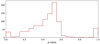 |
Fig. 1. Histogram of the computed p-values. BCGs that could not be fitted with a single component have a default p-value = 0, and those that could not be fitted with two components have a p-value = 1. |
3.2. Results
Out of the 1238 detected BCGs, 30 were not successfully fitted with either model, bringing our sample to 1208 galaxies. We then only considered galaxies with relative errors on the effective radius, mean surface brightness, and Sérsic index smaller than 20%. Excluding the objects with large uncertainties, we ended up with 1107 BCGs, of which 930 BCGs (84%) are well modelled with one Sérsic component and 177 BCGs (16%) are better modelled with two Sérsic components.
As in Chu et al. (2021), we also excluded all galaxies fitted with two Sérsics that have an inner component (the component with the smaller Re) that contributes more than 30% to the total luminosity of the galaxy. In the following we consider that the outer component of the double-Sérsic model contains most of the light in the galaxy. This will allow a comparison with a model with one Sérsic component.
Our final sample is thus made of 974 BCGs, of which 930 BCGs (95%) are better modelled with one Sérsic component and 44 BCGs (5%) with two Sérsic components. Among them, there are 80 blue BCGs (8%) which were all well modelled with a single Sérsic component. In the following we consider the measured properties of the outer component of the double-Sérsic BCGs, which is then compared to the properties of the single-Sérsic BCGs. We show the normalized redshift distribution of the sample for the two chosen models in Fig. 2. We find single-Sérsic BCGs at all redshifts, whereas we mainly find BCGs better fitted with two components at lower redshifts (77% of BCGs better fitted with two Sérsics are at redshift z < 0.4).
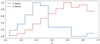 |
Fig. 2. Normalized histograms of the distribution of redshifts z for BCGs fitted with single-Sérsic (red) and double-Sérsic (blue) models. |
The histogram of the BCG Sérsic indices is shown in Fig. 3. The single-Sérsic model fits BCGs with all values of the Sérsic index n, and the distribution appears mostly flat. When a double-Sérsic model is required, the outer component has a very small value of n (mostly between 1 and 2) and the distribution appears more peaked.
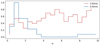 |
Fig. 3. Normalized histograms of the Sérsic indices n for BCGs fitted with single-Sérsic (red) and double-Sérsic (blue) models. For BCGs fitted with two components, we consider the Sérsic index of the outer component. |
Similar results were found in Chu et al. (2021). A first natural interpretation could be that as the redshift increases, the spatial resolution decreases. At lower redshifts, because the galaxies are better resolved, it is possible to distinguish the inner component from the outer component in some galaxies. As a result, galaxies at higher redshifts would be correctly fitted with a single profile, as the centre is not correctly resolved. However, Chu et al. (2021) show that this is not true: degrading the resolution of low-redshift BCGs to the resolution at z = 1 returns comparable results, implying that the models are resolution-independent. Moreover, we find similar distributions of z and n with the HST and CFHTLS samples, which strengthens our point, since the HST resolution is much higher than that of the CFHTLS.
We display in Fig. 4 the Sérsic index n as a function of the effective radius Re in logarithmic scale, colour-coded with redshift. Two-component BCGs are mainly concentrated in a zone with small Sérsic index (n < 2) and large effective radius (Re > 20 kpc), and they are also low-redshift objects (z < 0.4). When considering only those well fitted with one Sérsic, we find that the Sérsic indices increase as a function of the logarithm of the effective radius. Here, we find n = (5.13 ± 0.21)log(Re)+(−0.29 ± 0.26) (with a correlation coefficient R = 0.62 and significant with a p-value p ≪ 10−5)4. In the following, we consider R = 0.20 as the minimum value showing a faint trend, and define p = 0.05 as our significance level.
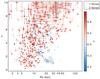 |
Fig. 4. Sérsic index n as a function of effective radius Re, colour-coded with redshift. Dots correspond to BCGs fitted with one Sérsic component and empty squares to BCGs fitted with two Sérsic components. For BCGs fitted with two components the properties of the outer component are considered. |
The absolute magnitude and effective radius as a function of redshift are displayed in Fig. 5. Absolute magnitudes range between −26 and −22 with no dependence on redshift. The effective radius is also redshift-independent. A very faint trend for BCGs to become brighter and bigger with redshift up to z = 1.8 is reported in Chu et al. (2021) (correlation coefficient R = −0.29 with a p-value p = 0.007 for the absolute magnitude to become brighter, and R = −0.40 in logarithmic scale with p < 10−3 for the size of BCGs to increase). Within the same redshift range as the present study, they measure no correlation for either of these two properties (R = 0.11 for the absolute magnitude and R = 0.27 for the effective radius, with p = 0.31 and p = 0.01 respectively). By increasing the sample size by more than a factor of ten, we therefore confirm that BCGs have not grown in luminosity or size since z = 0.7 (lower correlations R = 0.06 and R = 0.14, respectively, with p = 0.06 and p ≪ 0.05).
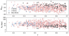 |
Fig. 5. Absolute magnitude (top) and effective radius (bottom) measured in the CFHTLS i filter, as a function of redshift. BCGs fit with a single component are represented by red dots, BCGs better fit with two components have their outer parameter represented by empty blue squares. Blue BCGs (see Sect. 2) are identified by dark stars. For BCGs fitted with two components the properties of the outer component are considered. |
The mean surface brightness, not corrected and corrected by a factor of (1 + z)4 for cosmological dimming, shows no significant dependence with redshift (Fig. 6). As a result, none of the measured parameters (brightness, surface brightness, size, Sérsic index) is observed to evolve with redshift up to z = 0.7.
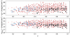 |
Fig. 6. Mean surface brightness as a function of redshift not corrected (top) and corrected (bottom) for cosmological dimming. The symbols are the same as in Fig. 5. For BCGs fitted with two components the surface brightness of the outer component is considered. |
Blue BCGs, identified by dark stars in the previous figures, also do not show any signs of evolution, but they seem to occupy preferential locations in these relations. For the most part, blue BCGs tend to be at higher redshifts (76% at z > 0.5), less bright (mean absolute magnitude for blue BCGs Mabs, i, blue = −23.5, for red BCGs Mabs, i, red = −24.2), and smaller (mean effective radius for blue BCGs Re, blue = 8 kpc, for red BCGs Re, red = 22 kpc) (see Fig. 5), and to have brighter mean surface brightnesses than their red BCG counterparts (mean surface brightness for blue BCGs μblue = 22.1, for red BCGs μred = 22.6) (see Fig. 6).
3.3. Kormendy relation for BCGs
The Kormendy relation (Kormendy 1977) between the mean surface brightness and the effective radius is shown in Fig. 7 before (left) and after (right) correcting for the (1 + z)4 cosmological dimming effect. With more than 1000 objets, here the Kormendy relation is very well defined (R > 0.88, p = 0). Without correction for cosmological dimming, we measure the relation as ⟨μ⟩ = (3.34 ± 0.05)log Re + (18.65 ± 0.07). Similarly to Bai et al. (2014) and Chu et al. (2021), we find that the slope of the Kormendy relation stays constant with redshift. The relation is also independent of the model used (single- or double-Sérsic profiles).
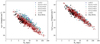 |
Fig. 7. Kormendy relation before (left) and after (right) correcting for cosmological dimming. The symbols with various colours correspond to different redshift intervals. For BCGs fitted with two components we consider the properties of the outer component. |
After correcting for cosmological dimming, we find ⟨μ⟩ = (3.49 ± 0.04)log Re + (16.72 ± 0.05). This removes the redshift dependence observed in the left figure, and tightens the relation observed.
3.4. Properties of the double-Sérsic BCG inner component
As in Chu et al. (2021), we do not find any correlation for any of the properties of the inner component of the double-Sérsic BCGs with redshift. The similar sample sizes of about 40 BCGs in Chu et al. (2021) and the present paper do not enable us to better constrain the inner part of these galaxies, and we do not have good enough statistics for our analysis to become significant. Even so, we note that compared to the outer component, the inner component tends to be brighter by at least one magnitude (we recall the selection criterion we applied on double-Sérsic BCGs to retain only those with an inner component that does not contribute much to the total luminosity of the galaxy) and tends to be smaller in size by at least a factor of 3.
The Kormendy relation is also very well defined for the inner component at smaller effective radii and brighter mean surface brightnesses (R = 0.93, p ≪ 0.05) than the relation illustrated in Fig. 7. For the inner component, the relation uncorrected for cosmological dimming is ⟨μ⟩ = (4.69 ± 0.29)log Re + (17.94 ± 0.15).
4. Effect of the ICL on luminosity profiles of galaxies
Despite its faint nature, the ICL may contribute in the outskirts of BCGs and have an influence on their luminosity profiles at large radii. We try here to quantify how much the ICL affects the BCG profiles in model fitting.
We make use of the ICL and background images, kindly provided by Y. Jimenez-Teja, to estimate the effect of the ICL on the shape and photometry measured by GALFIT. Jiménez-Teja et al. (2018) study the ICL fraction in a sample of clusters from the CLASH and Frontier Fields (FF) surveys observed with the HST. We compared the fits obtained with GALFIT on the original HST images with those obtained after subtracting the ICL using the maps provided by Y. Jimenez-Teja. We prefer to use these HST data rather than our current CFHTLS sample for this study as we have spectroscopic redshifts available for the HST sample, better spatial resolution, and the clusters studied in Jiménez-Teja et al. (2018) have deep images on which the ICL was well studied and detected. To check which model between the single-Sérsic and the double-Sérsic models fits our galaxies best, the BCGs are first modelled with GALFIT on the original images. We find that all BCGs need a second component according to the F-test described in Sect. 3.
We then subtract the ICL and background from our images and run GALFIT on these final images, which only contain the BCG. We then compare the returned parameters, and check if subtracting the ICL allows us to remove the inner component needed on the original images. This should indeed allow us to understand if the double-Sérsic model BCGs observed mostly at low redshifts (z ≤ 0.4) are an effect of the ICL being more easily detectable at lower z.
From a sample of 11 clusters up to z = 0.54, four BCGs could not be fitted properly with GALFIT with one or two components. The remaining seven clusters studied here are shown in Table 1. We find that all BCGs, even after subtracting the ICL, are still better fitted using two Sérsic profiles. Thus, we deduce that the ICL does not affect the inner structure of the galaxy, and the need for a second component is not caused by the ICL. By comparing the parameters obtained on the original and ICL subtracted images, by letting all parameters free in GALFIT, we found that the presence of the ICL could disturb the profile of the outer component of the model (in particular, higher effective radius by about a factor of two or three). To better estimate how much the ICL can affect our models, we chose to model one more time the BCGs on the original images, but we fixed the inner component with the parameters obtained on the images without ICL. As the ICL mainly affects the outskirts of the profile, the inner region of the BCG is supposed to be hardly modified. By fixing the inner component, we make sure that we only take into account the differences caused by the ICL.
Sample of the seven clusters from Jiménez-Teja et al. (2018) studied and successfully modelled with GALFIT.
The parameters measured with two components can be found in Table 2. For all seven BCGs, the absolute magnitude MABS of the external component is brighter after removing the ICL (with a difference ΔMABS ≤ 2). After subtracting the ICL, the BCGs also have brighter effective surface brightness values, with Abell 2744 presenting the biggest difference of almost 3 mag/arcsec2. Additionally, for all cases, the effective radii increase in the presence of ICL, some of them drastically. The measured effective radius can be up to 13 times bigger when the ICL is still present in the images. This is the case for MACS J1149+2223.
Parameters obtained from fitting the luminosity profiles with two Sérsic components for the ICL sample.
To further illustrate this, we plot the Kormendy relation obtained with the seven BCGs, before and after subtracting the ICL (Fig. 8). The relation after subtracting the ICL is shifted at lower Re and brighter ⟨μ⟩, which is consistent with our previous remarks. The slope of the Kormendy relation does not depend on the presence of the ICL.
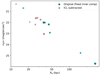 |
Fig. 8. Kormendy relation obtained for the seven BCGs in our sample before (blue) and after (red) subtracting the ICL on the original images. Each cluster is represented by a different symbol. |
The outer component profile on ICL-subtracted images still presents a low Sérsic index with n < 2 for all BCGs. The Sérsic indices without ICL are smaller than those measured with ICL, resulting in a flatter profile in the outskirts. This is to be expected, as the ICL would extend the profile at higher radii with very faint surface brightness, and the stars that constitute the ICL would blend with the stars that are bound to the BCG in the outskirts. The galaxy would thus appear less compact, bigger, and more diffuse in the presence of ICL.
Since the component with very low Sérsic index (n < 2) is still present even after removing the ICL from the original images, we thus conclude that the dichotomy observed in the distribution of Sérsic indices and redshifts, following the best model used, is not related to the ICL. Drawing any conclusions regarding the evolution of the size of BCGs with redshift can be tricky, however, as the ICL can affect the profile at large radius.
We tried to take the ICL into account by adding a third Sérsic profile when fitting the original images, and by fixing the parameters of the first two components to those obtained on the ICL subtracted images. Although a Sérsic profile might not be the best choice to model the ICL, our goal was only to check if GALFIT would be able to detect a third component in addition to the BCG. If successful, we could then try to fit three Sérsic profiles instead of two to our whole sample in order for it not to be affected by the ICL contribution.
The test was done on the cluster RX J2129 (chosen arbitrarily from the BCGs that were well fitted previously). A third component was successfully detected and was modelled with faint surface brightness (μICL = 25.24), large effective radius (Re, ICL = 190 kpc, i.e. more than four times bigger than that of the outer component), and very low Sérsic index (n = 0.4). Though this result was expected, as the ICL is by nature a very extended envelope with faint surface brightness, GALFIT returns a very elongated component (b/a = 0.2), whereas the ICL map appears close to circular. We thus conclude that GALFIT does not manage to correctly model the ICL and has difficulties in properly fitting components with very faint surface brightness. Adding a third component, in addition to being even more time consuming, is not possible with GALFIT to correct for the effect of the ICL on the outer profile of BCGs.
5. Effect of the depth of the images
As demonstrated above, the presence of BCGs with two Sérsic components observed mostly at low redshifts (z < 0.4) is neither due to the lower resolution at higher redshifts nor to the presence of ICL at low redshifts. In Chu et al. (2021), we degraded the resolution of low-redshift clusters to that at redshift z = 1 and in Sect. 4 we remove the ICL from our images to check if these two parameters can influence the choice of the best fitting model, according to the F-test. In both cases we found that we still need two components to properly fit the BCGs that were better modelled with two Sérsics on the original images.
Although we increased by more than a factor of ten the sample size up to z = 0.7 from Chu et al. (2021), we find similar numbers for galaxies better fitted by two Sérsic profiles. Either this is related to the evolution of BCGs, or another observational bias comes into play. To confirm this, we study how the depth of the images affects the model distribution shown in Fig. 2 and in Chu et al. (2021).
We measure the magnitude at 80% completeness, m80, of our catalogues and show the distribution of the model chosen as a function of m80 (see Fig. 9). The images in Chu et al. (2021) obtained with HST are deeper than those used in the present study, based on the CFHTLS. In Chu et al. (2021, Fig. 9, bottom plot) the distribution of m80 has a peak at m80 = 25.4, and can reach m80 = 28.0. With our CFHTLS sample, we measure a peak at m80 = 24.7 (Fig. 9, top plot), and no cluster has m80 > 25.5. This is consistent with the value indicated in the TERAPIX documentation5.
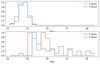 |
Fig. 9. Normalized distributions of the magnitudes at 80% completeness for the sample in this paper (top) and in Chu et al. (2021, bottom). The red histograms represent BCGs well fitted with a single component; blue histograms are BCGs better fitted with two components. |
With the HST data, out of 54 BCGs up to z = 0.7, 37 (69%) were better modelled with two Sérsics. BCGs better modelled with two components have images that go deeper than m80 = 25.2. For the deepest images (m80 > 26.5), the BCGs that need an additional component become dominant. Only one BCG was well fitted with a single Sérsic; the other 13 BCGs in that redshift range were better fitted with the more complex model. In the present study, in the same redshift range, we find that only 5% of BCGs need an additional component. Not only does the depth of the CFHTLS images not go as deep as the HST images, but it is also limited to a magnitude m80 = 25, which is below the magnitude of the peak measured for HST for those fitted with two components. We can guess that if deeper images were available for the CFHTLS, the structure of the BCGs would be better resolved and the number of two-component BCGs would increase.
In another attempt to highlight the influence of the depth of the images on the model used to fit the BCGs, we made use of the Deep fields of the CFHTLS. Eight BCGs in our sample were observed both in the Wide and Deep surveys, allowing us to compare directly the effect of the depth of the images on the luminosity profiles of the BCGs. Using the Deep survey, we find that six out of eight BCGs have a two-component structure. On the other hand, all but one of the same objects observed in the Wide survey lack an inner component. Additionally, the p-values computed on the Wide images (pW > 0.35 on average) are much higher than those obtained on the Deep images (pD < 0.1), indicating that the residuals of the two models tend to become similar as the images become shallower. For one BCG still lacking an inner component on the Deep image, the Wide p-value (pW = 0.59) drops to pD = 0.18 for the Deep image. This suggests that an even deeper image would allow us to resolve the inner component that is currently ‘hidden’. This BCG is also the farthest galaxy in our sample of eight BCGs, at z = 0.65. On the contrary, the BCG that was better modelled with two components in both images is the one at the lowest redshift, z = 0.19.
It may be important to note that in Chu et al. (2021), double-Sérsic BCGs are also observed at redshifts higher than z > 0.4. Although they are more dominant at lower redshifts and not as much at higher redshift, we still account for two-component galaxies up to z = 1.8. By plotting a z − m80 diagram, we distinguish two populations at z > 0.7. The first is the dominant population of single-Sérsic BCGs at z > 0.7, modelled on images with m80 < 26 mag arcsec−2; the second is the population of double-Sérsic BCGs, modelled on images with m80 > 27 mag arcsec−2. Consequently, if deeper surveys were available, we could assume that not only would the fraction of two-component BCGs increase at low redshifts, but this would happen at higher redshifts as well.
We also checked if the ICL could be detected in our images, and thus if the ICL affects our study, by measuring its surface brightness on the images provided by Jiménez-Teja et al. (2018) and comparing it with the limit computed for the CFHTLS images. We were able to do this, as images provided by Jiménez-Teja et al. (2018) are very deep images limited to magnitude 27.7 in the F814W ACS filter. Taking the example of RX J2129, the profile in surface brightness is shown in Fig. 10. We find a maximum surface brightness of 26 mag arcsec−2 in the centre of the cluster. The profile becomes dimmer the farther we go from the centre, and reaches a surface brightness of 28 mag arcsec−2 at distances r > 0.7 arcsec (r > 2.6 kpc) from the centre. When compared to the surface brightness limit of our CFHTLS sample (μCFHTLS, 80 = 21.5 mag arcsec−2), the ICL is too faint to be observed in our images. We measured a surface brightness μICL = 26 mag arcsec−2 for the ICL, which is fainter than the surface brightness limit measured on the CFHTLS images. We can thus confirm that the results shown previously are physical and are not affected by ICL.
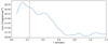 |
Fig. 10. Surface brightness profile of the ICL in the cluster RX J2129. The surface brightness was computed in a circular aperture, centred on the cluster centre, with a radius r. The red vertical line represents the Kron radius of the BCG. |
6. Alignment of BCGs with their host clusters
With the purpose of studying the alignment of BCGs with their host clusters, we measured their positions angles (PA) and ellipticities with GALFIT. Out of the 974 BCGs that were fitted by either one or two Sérsic profiles, 126 have a minor-to-major axis ratio b/a ≥ 0.9. As in Chu et al. (2021), we exclude these galaxies as an ellipticity close to unity leads to high uncertainties on the measurement of the PA, and also to an ill-defined PA. We thus end up with 848 BCGs.
We measured the cluster ellipticities by fitting ellipses on the density maps with a 3σ clipping, applying the ellipse function in the Python photutils package6. All clusters with b/a ≥ 0.9 were excluded. This reduced the sample to 639 clusters.
Similarly to West et al. (2017), we measured the PA of clusters by computing the moments of inertia on the galaxy density maps provided by Sarron et al. (2018), and estimated the uncertainties with bootstrap resamplings. For each cluster, we generated 100 bootstraps of half of the pixels of the density maps, in a radius R500, c corresponding to the radius within which the mean density is 500 times the critical density of the Universe at the redshift of the cluster, ρc(z). The size of R500, c was computed from the R200, c radius obtained for each cluster in Sarron et al. (2018). The conversion was done using the relation given in Sun et al. (2009): R500, c = 0.669 R200, c. This R200, c was derived from the M200 estimate of Sarron et al. (2018) inferred from an X-ray derived mass to optical richness scaling relation:
We initially wanted to exclude all clusters that present large uncertainties on their PAs. However, we found that most clusters tend to have very high uncertainties of around 45 degrees. This can be explained by the fact that, as stated in Sect. 2, clusters are detected in density maps that cover a wide redshift bin (on average, the width of the redshift bin is δz = 0.15), which means one detection can overlap with another cluster at a nearby redshift. The presence of filaments, which link clusters in the cosmic web, can also bias the measured PA. For all these reasons, the uncertainties computed by bootstrap resampling can be large if the cluster is not rich (and thus has a low S/N on density maps), if it is circular, or if it is not isolated.
We chose to cut the samples by removing clusters with uncertainties bigger than 45, 40, and 35 degrees. This reduced our samples to 420, 203, and 116 clusters and BCGs, respectively.
The alignments (differences between the cluster and BCG PAs) for the final samples are illustrated in Fig. 11. For all three histograms, even with the largest uncertainties on the PA of the cluster, we still observe a peak at lower differences. We measure, respectively (for errors of 45, 40, and 35 degrees), 44 ± 2%, 51 ± 3%, and 57 ± 4% of BCGs aligned within 30 degrees with their host clusters (uncertainties on the alignment fractions were computed by bootstrap resampling). On the contrary, only 24%, 22%, and 18% of BCGs differ by more than 60 degrees from the major axis of the cluster. This shows a tendency for BCGs to align with the major axis of their host clusters that is discussed in Sect. 7. To assess the confidence that our observation is not due to random fluctuations in a sample with a finite number of clusters, we computed the expected uncertainty on frandom through bootstrap realisations of sampling from a random distribution for N = 420 and 116 clusters, respectively. This allows us to estimate that the observed alignment is not due to random fluctuations at 3.4σ (ΔPAcluster < 45 deg) and 4σ (ΔPAcluster < 35 deg), respectively.
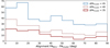 |
Fig. 11. Histograms of the alignments (absolute difference of PAs) between BCGs and their host clusters. The histograms were obtained after excluding circular objects and systems, and excluding clusters with large PA uncertainties (ΔPAcluster > 45 degrees in blue, ΔPAcluster > 40 degrees in light red, ΔPAcluster > 35 degrees in dark red). |
Furthermore, we find that BCGs in very massive clusters of Mcluster > 5 1014 M⊙ (and thus the most massive BCGs, by converting cluster mass to BCG mass using the relation given in Bai et al. 2014), and bigger BCGs with Re, BCG > 30 kpc, tend to be better aligned than the less massive ones. All BCGs in that size and mass range, from Chu et al. (2021, 2 BCGs) and in the present paper (12 BCGs), are found to be better aligned than 30 degrees with the major axis of their host clusters. It is difficult to confirm this with less massive galaxies, however, because of the large scatter in the Mcluster versus |PAcluster – PABCG| relation (similarly, MBCG versus |PAcluster – PABCG|) and the Re, BCG versus |PAcluster – PABCG| relations.
7. Discussion and conclusions
Making use of the galaxy cluster catalogue of Sarron et al. (2018), we developed an algorithm to detect BCGs in optical images from the CFHTLS. We estimate that 70% of the BCGs in our sample were successfully detected. The final sample of BCGs built and studied in this paper consists of 1238 BCGs.
This method requires large images in order to properly estimate the background (at least 2 Mpc to be far enough from the cluster centre), as well as images in several filters to obtain a good photometric redshift estimate of the galaxies in the cluster field. With the CFHTLS, five filters were available to fit the objects with the LePhare code, enabling Sarron et al. (2018) to estimate photometric redshifts with a typical accuracy of 0.05 × (1 + z).
Several studies such as McDonald et al. (2016), Cerulo et al. (2019), Fogarty et al. (2019), Castignani et al. (2020) and Chu et al. (2021) have identified BCGs with unusual blue colours, showing signs of recent starbursts. However, such BCGs are scarce, and increasing their statistics is necessary to better understand the processes that lead these galaxies to behave differently from their red counterparts. By computing the (g − i) colours of the BCGs, we also estimate the fraction of blue (g − i < 0) BCGs in the Universe up to z = 0.7. We find that 9% of BCGs in our sample are blue, which is consistent with the estimates given in the cited papers.
By applying the same method as in Chu et al. (2021), we modelled the luminosity profiles of the BCGs by fitting two models, one with a single Sérsic component and one with two Sérsic components. The model was chosen using the statistical F-test: we observed two populations with a separation at z = 0.4, below which some BCGs tend to require an additional component to take into account the brighter bulge. Up to z = 0.7, in Chu et al. (2021), we found that 77% of BCGs were better modelled with two components, while here only 5% are better modelled with two Sérsics in the same redshift range. Even though we significantly increase the size of our sample, the number of two-component BCGs did not increase, and we find that the fraction of double-Sérsic BCGs actually decreases. In order to understand and explain why these galaxies with a more important bulge exist mostly at lower redshifts, we checked for any observational bias that could affect our study.
Although the spatial resolutions of this sample and of the sample in Chu et al. (2021) are different, we still find similar distributions for the best model, with double-Sérsic BCGs found mainly at lower redshifts (z < 0.4). We also find similar distributions for the Sérsic indices, with two-component BCGs having lower indices (n < 2), and single-component BCGs presenting indices that cover a wide range between 0 and 10, with a flatter distribution. This hints that the resolution of the images does not play a large role in model fitting. We confirmed this in Chu et al. (2021) by degrading the resolution of HST images at low z and verifying that the fits returned by GALFIT were unchanged.
We already took into account the distance at which the galaxies are observed by considering a filter that is above the 4000 Å break, and thus by always modelling the same red stellar population. However, it is all the more difficult to detect objects with faint surface brightness at high redshifts, without deep exposure times. We thus pondered if ICL, which has very faint surface brightness, might be detectable at lower redshifts, and would thus constitute the second component observed.
By removing the ICL contribution, using images provided by Jiménez-Teja et al. (2018), we show that the presence of ICL can affect the outskirts of the galaxy, and can flatten the profiles at large radii. The presence of ICL can decrease the outer Sérsic index, and increase the size of the BCG. Nonetheless, a second component with low Sérsic index is still needed even after subtracting the ICL. The presence of double-Sérsic BCGs with low index at low redshift is thus also not an effect of the ICL. Moreover, the images studied here are not deep enough to detect the ICL, which is too faint, with a surface brightness μICL ≥ 26 mag arcsec−2. We conclude that our study is not affected by the presence of ICL.
It should be noted that Kluge et al. (2020, 2021), who study a sample of 170 local BCGs up to z = 0.08, find a fraction of 71% of BCG+ICL systems that are well described with a single Sérsic component. The remaining 29% are better fitted with an additional component. This outer component of the double-Sérsic BCG+ICL system would trace the unrelaxed star material that might have been accreted in the recent past.
In this study we find that 95% of the BCGs in our sample at higher redshifts are well modelled with a single Sérsic component, and 5% need two components. The very different fractions between the two studies could be due to the depth of the images and/or to the presence of ICL. The limiting magnitude in Kluge et al. (2020, 2021) is deeper, SBlim = 30 g′ mag arcsec−2, which allows them to detect the ICL surrounding the BCG. In the present study the magnitude at 80% completeness in the i CFHTLS filter is m80 = 24.7. We also show for a small sample of seven BCGs from Jiménez-Teja et al. (2018) that the presence of a second component is independent from the presence of ICL. If the ICL does not play a role in the existence of a second component, then it cannot explain the difference between Kluge et al. (2020, 2021) and our study. A large sample of BCGs with deep images, as in Kluge et al. (2021), should be used to disentangle the ICL contribution with a similar method to the one we applied to the ICL-subtracted images from Jiménez-Teja et al. (2018).
Lastly, we compare the completeness of our catalogues. We recall that in Chu et al. (2021) 85% of BCGs at redshift z ≤ 0.4 are two-component galaxies, whereas here they only represent 16% of our sample at z ≤ 0.4. We find that double-Sérsic component BCGs in Chu et al. (2021) tend to appear in images that have a depth of the order of m80 > 26.5 mag arcsec−2. Our current CFHTLS data do not go as deep as the HST images, and the structure of the BCG is thus not as well determined. We could assume that repeating this study with deeper images would reveal the existence of an inner component at z ≤ 0.4 for most of the BCGs that are well modelled with a single Sérsic component in this paper. The presence of such an inner structure would indicate that bulges of BCGs may have formed first, and the extended envelope would have formed later on, at z ≤ 0.4. As Edwards et al. (2019) state, the cores and inner regions of BCGs were already formed long ago and stopped evolving, whereas the outer regions as well as the ICL started developing recently via minor mergers. This would also agree with the assumption that the ICL was formed at later times (z < 1.0), as stated by Jiménez-Teja et al. (2018) and references therein. Montes & Trujillo (2017) claim that the ICL saw most of its formation happen at z = 0.5; this would agree with the discrepancy between the two models we observe around z = 0.4, which could hint at a more important contribution of the ICL to the luminosity profile of BCGs at z ≤ 0.4. According to Lauer et al. (2014), from a study of 433 z ≤ 0.08 BCGs, although the inner portions would have already been assembled before the cluster was formed, the envelope would be expanded by dry mergers as the BCG spends time in the dense centre of the cluster. These dry mergers would not make the BCG brighter, but they would contribute greatly to the extension of its outer envelope. This inside-out scenario has been confirmed by many authors (De Lucia & Blaizot 2007; van Dokkum et al. 2010; Bai et al. 2014; Ragone-Figueroa et al. 2018; Edwards et al. 2019; Dalal et al. 2021). As they experience more interactions with other galaxies, and thus as their envelope forms as they accrete more and more matter, BCGs can be expected to evolve from single-Sérsic into double-Sérsic BCGs.
In Chu et al. (2021), double-Sérsic BCGs are observed up to z = 1.8, even though they are not dominant at higher redshifts. These two-component galaxies are found in the deepest images with limiting magnitudes m80 > 27 mag arcsec−2. The remaining population of single-Sérsic BCGs are modelled on images with m80 < 26 mag arcsec−2. The separation between the two models at higher redshifts that depends on the depth of the images highlights the importance of deep surveys. We would expect to detect two components in all BCGs, but this requires deep images and long exposure times. Even though the depth of the images could be a solution to resolving the structure of these central galaxies, we can still wonder if other cluster properties may be linked to the properties of this inner component. We do not find any correlation between the properties of the inner component and redshift, or with the cluster properties. Moreover, the small sample size of double-Sérsic BCGs does not enable us to draw any significant conclusions. Deeper surveys are needed to confirm our results and assumptions, and determine any link between the presence of an inner component and BCG growth.
In order to understand whether BCGs are still growing today, we looked for correlations between redshift and the physical properties of BCGs measured with GALFIT. We find no evolution as a function of redshift for the effective radius and absolute magnitude. In Chu et al. (2021), no correlation could be found for the mean surface brightness when no dimming correction was applied, up to z = 1.8. A trend could be seen up to z = 0.7 (R = 0.29, p = 0.013), but in fact this trend was caused by cosmological dimming. After correcting for this effect, the trend is no longer measured (R < 0.1). We once again verified this result, as no correlation could be found here between the corrected mean surface brightness and redshift. The large size of our sample enables us to confirm the results shown in Chu et al. (2021) up to z = 0.7, namely that BCGs were mainly formed before 0.7 (z = 1.8 in our previous study), and have properties that appear to have remained stable since then.
Following the work of Graham & Colless (1997) and Bai et al. (2014), we demonstrate that the Sérsic index varies as the logarithm of the effective radius: n = (5.13 ± 0.21)log(Re) +(−0.29 ± 0.26), while Graham & Colless (1997) find approximately n ∝ 3.22 log(Re). Our relation is steeper than that found by these authors, which means the measured Sérsic indices are more sensitive to small variations of the effective radius.
We also plot the Kormendy relation for BCGs, which is very well defined with our sample. Our relation, not corrected for cosmological dimming, ⟨μ⟩ = (3.34 ± 0.05)log Re + (18.65 ± 0.07), agrees within 1σ with that given in Bai et al. (2014) and Chu et al. (2021), and within 3σ with Durret et al. (2019):
⟨μ⟩ = (3.50 ± 0.18)log Re + (18.01 ± 0.23) (Bai et al. 2014);
⟨μ⟩ = (3.33 ± 0.73)log Re + C (Chu et al. 2021);
⟨μ⟩ = (2.64 ± 0.35)log Re + (19.7 ± 0.5) (Durret et al. 2019).
The dependence with redshift is due to cosmological dimming, which moves the relation to fainter surface brightnesses without affecting the sizes of the BCGs. The slope measured is also steeper than that of Bai et al. (2014) measured for non BCG early type galaxies: ⟨μ⟩ = (2.63 ± 0.28)log Re + C.
Following the work of Donahue et al. (2015), West et al. (2017), Durret et al. (2019), De Propris et al. (2020) and Chu et al. (2021), we show that the major axis of the BCG tends to align with that of the host cluster. We find that at least (44 ± 2)% of BCGs are aligned with their host clusters within 30 degrees. By only considering the best measured PAs (uncertainties smaller than 35 degrees), this percentage goes up to (57 ± 4)%. If BCGs had a random orientation, we would expect a uniform distribution, and thus only frandom = 33% of BCGs aligned with the major axis of their host clusters within 30 degrees. We confirm that the measured alignment fractions are not due to random fluctuations as the number of clusters studied is finite. We also confirm the results by Faltenbacher et al. (2009), Niederste-Ostholt et al. (2010) and Hao et al. (2011) who find stronger alignments for brighter and bigger galaxies. In the hierarchical scenario of structure formation, matter and galaxies fall into the centre of clusters along cosmic filaments. This would create tidal interactions that can explain the observed alignment of BCGs with their host clusters. Thus, contrary to other cluster members, as was found by West et al. (2017) who show that non BCGs members of a cluster have a random orientation in the cluster, the BCG properties are linked to the cluster.
This study shows, with increased statistics, evidence for an early formation of the brightest central galaxies in clusters. Most of their matter content was already in place by z = 0.7, and we showed in Chu et al. (2021) that this conclusion can most likely be applied up to z = 1.8. New datasets in the infrared (JWST, Euclid) should enable us to confirm this result at higher redshifts with better statistics. In the present paper, we also estimate in a first approach the contribution of the ICL to such studies.
Linear regressions were made using the Python scipy lingress function: https://scipy.org/
Acknowledgments
We are very grateful to Y. Jiménez-Teja for providing us with her ICL images. We also thank A. Ellien for discussions on the ICL. We thank the referee for her/his constructive comments and suggestions. F.D. acknowledges continuous support from CNES since 2002. I.M. acknowledges financial support from the State Agency for Research of the Spanish MCIN through the “Center of Excellence Severo Ochoa” award to the Instituto de Astrofísica de Andalucía (SEV-2017-0709), and through the program PID2019-106027GB-C41. Based on observations obtained with MegaPrime/MegaCam, a joint project of CFHT and CEA/DAPNIA, at the Canada-France-Hawaii Telescope (CFHT) which is operated by the National Research Council (NRC) of Canada, the Institut National des Sciences de l’Univers of the Centre National de la Recherche Scientifique (CNRS) of France, and the University of Hawaii. This work is based in part on data products produced at Terapix and the Canadian Astronomy Data Centre as part of the Canada-France-Hawaii Telescope Legacy Survey, a collaborative project of NRC and CNRS. This research has made use of the NASA/IPAC Extragalactic Database (NED) which is operated by the California Institute of Technology, under contract with the National Aeronautics and Space Administration.
References
- Adami, C., Sarron, F., Martinet, N., & Durret, F. 2020, A&A, 639, A97 [NASA ADS] [CrossRef] [EDP Sciences] [Google Scholar]
- Arnouts, S., Cristiani, S., Moscardini, L., et al. 1999, MNRAS, 310, 540 [Google Scholar]
- Ascaso, B., Aguerri, J. A. L., Varela, J., et al. 2010, ApJ, 726, 69 [Google Scholar]
- Bai, L., Yee, H., Yan, R., et al. 2014, ApJ, 789, 134 [Google Scholar]
- Bernardi, M. 2009, MMNRAS, 395, 1491 [NASA ADS] [CrossRef] [Google Scholar]
- Bertin, E. in Astronomical Data Analysis Software and Systems XX, eds. I. N. Evans, A. Accomazzi, D. J. Mink, & A. H. Rots, ASP Conf. Ser., 442, 435 [Google Scholar]
- Binggeli, B. 1982, A&A, 107, 338 [NASA ADS] [Google Scholar]
- Bruzual, G., & Charlot, S. 2003, MNRAS, 344, 1000 [NASA ADS] [CrossRef] [Google Scholar]
- Castignani, G., & Benoist, C. 2016, A&A, 595, A111 [NASA ADS] [CrossRef] [EDP Sciences] [Google Scholar]
- Castignani, G., Pandey-Pommier, M., Hamer, S. L., et al. 2020, A&A, 640, A65 [NASA ADS] [CrossRef] [EDP Sciences] [Google Scholar]
- Cerulo, P., Orellana, G. A., & Covone, G. 2019, MNRAS, 487, 3759 [Google Scholar]
- Chu, A., Durret, F., & Márquez, I. 2021, A&A, 649, A42 [NASA ADS] [CrossRef] [EDP Sciences] [Google Scholar]
- Cui, W., Murante, G., Monaco, P., et al. 2014, MNRAS, 437, 816 [Google Scholar]
- Dalal, R., Strauss, M. A., Sunayama, T., et al. 2021, MNRAS, 507, 4016 [NASA ADS] [CrossRef] [Google Scholar]
- De Lucia, G., & Blaizot, J. 2007, MNRAS, 375, 2 [Google Scholar]
- De Propris, R., West, M. J., Andrade-Santos, F., et al. 2020, MNRAS, 500, 310 [Google Scholar]
- Donahue, M., Connor, T., Fogarty, K., et al. 2015, ApJ, 805, 177 [Google Scholar]
- Durret, F., Tarricq, Y., Márquez, I., Ashkar, H., & Adami, C. 2019, A&A, 622, A78 [NASA ADS] [CrossRef] [EDP Sciences] [Google Scholar]
- Edwards, L. O. V., Salinas, M., Stanley, S., et al. 2019, MNRAS, 491, 2617 [Google Scholar]
- Ellien, A., Slezak, E., Martinet, N., et al. 2021, A&A, 649, A38 [NASA ADS] [CrossRef] [EDP Sciences] [Google Scholar]
- Faltenbacher, A., Li, C., White, S. D. M., et al. 2009, Res. Astron. Astrophys., 9, 41 [Google Scholar]
- Fogarty, K., Postman, M., Li, Y., et al. 2019, ApJ, 879, 103 [Google Scholar]
- Graham, A., & Colless, M. 1997, MNRAS, 287, 221 [Google Scholar]
- Hao, J., Kubo, J. M., Feldmann, R., et al. 2011, ApJ, 740, 39 [NASA ADS] [CrossRef] [Google Scholar]
- Henriques, B. M. B., White, S. D. M., Lemson, G., et al. 2012, MNRAS, 421, 2904 [Google Scholar]
- Ilbert, O., Arnouts, S., McCracken, H. J., et al. 2006, A&A, 457, 841 [NASA ADS] [CrossRef] [EDP Sciences] [Google Scholar]
- Jiménez-Teja, Y., & Dupke, R. 2016, ApJ, 820, 49 [Google Scholar]
- Jiménez-Teja, Y., Dupke, R., Benítez, N., et al. 2018, ApJ, 857, 79 [Google Scholar]
- Jiménez-Teja, Y., Vílchez, J. M., Dupke, R. A., et al. 2021, ApJ, 922, 268 [CrossRef] [Google Scholar]
- Kluge, M., Neureiter, B., Riffeser, A., et al. 2020, ApJS, 247, 43 [Google Scholar]
- Kluge, M., Bender, R., Riffeser, A., et al. 2021, ApJS, 252, 27 [Google Scholar]
- Kormendy, J. 1977, ApJ, 218, 333 [NASA ADS] [CrossRef] [Google Scholar]
- Lauer, T. R., Postman, M., Strauss, M. A., Graves, G. J., & Chisari, N. E. 2014, ApJ, 797, 82 [Google Scholar]
- Margalef-Bentabol, B., Conselice, C. J., Mortlock, A., et al. 2016, MNRAS, 461, 2728 [Google Scholar]
- Márquez, I., Durret, F., Delgado, R. G., et al. 1999, A&AS, 140, 1 [NASA ADS] [CrossRef] [EDP Sciences] [Google Scholar]
- Márquez, I., Masegosa, J., Durret, F., et al. 2003, A&A, 409, 459 [NASA ADS] [CrossRef] [EDP Sciences] [Google Scholar]
- McDonald, M., Stalder, B., Bayliss, M., et al. 2016, ApJ, 817, 86 [Google Scholar]
- Montes, M., & Trujillo, I. 2017, MNRAS, 474, 917 [Google Scholar]
- Niederste-Ostholt, M., Strauss, M. A., Dong, F., Koester, B. P., & McKay, T. A. 2010, MNRAS, 405, 2023 [NASA ADS] [Google Scholar]
- Ragone-Figueroa, C., Granato, G. L., Ferraro, M. E., et al. 2018, MNRAS, 479, 1125 [NASA ADS] [Google Scholar]
- Sarron, F., & Conselice, C. J. 2021, MNRAS, 506, 2136 [NASA ADS] [CrossRef] [Google Scholar]
- Sarron, F., Martinet, N., Durret, F., & Adami, C. 2018, A&A, 613, A67 [NASA ADS] [CrossRef] [EDP Sciences] [Google Scholar]
- Schlafly, E. F., & Finkbeiner, D. P. 2011, ApJ, 737, 103 [Google Scholar]
- Schlegel, D., Finkbeiner, D., & Davis, M. 1998, ApJ, 500, 525 [Google Scholar]
- Springel, V., White, S. D. M., Jenkins, A., et al. 2005, Nature, 435, 629 [Google Scholar]
- Stott, J. P., Collins, C. A., Burke, C., Hamilton-Morris, V., & Smith, G. P. 2011, MNRAS, 414, 445 [Google Scholar]
- Sun, M., Voit, G. M., Donahue, M., et al. 2009, ApJ, 693, 1142 [NASA ADS] [CrossRef] [Google Scholar]
- Thomas, D., Maraston, C., Schawinski, K., Sarzi, M., & Silk, J. 2010, MNRAS, 404, 1775 [NASA ADS] [Google Scholar]
- van Dokkum, P. G., Whitaker, K. E., Brammer, G., et al. 2010, ApJ, 709, 1018 [Google Scholar]
- West, M. J., de Propris, R., Bremer, M. N., & Phillipps, S. 2017, Nat. Astron., 1, 0157 [Google Scholar]
All Tables
Sample of the seven clusters from Jiménez-Teja et al. (2018) studied and successfully modelled with GALFIT.
Parameters obtained from fitting the luminosity profiles with two Sérsic components for the ICL sample.
All Figures
|
Fig. 1. Histogram of the computed p-values. BCGs that could not be fitted with a single component have a default p-value = 0, and those that could not be fitted with two components have a p-value = 1. |
| In the text | |
|
Fig. 2. Normalized histograms of the distribution of redshifts z for BCGs fitted with single-Sérsic (red) and double-Sérsic (blue) models. |
| In the text | |
|
Fig. 3. Normalized histograms of the Sérsic indices n for BCGs fitted with single-Sérsic (red) and double-Sérsic (blue) models. For BCGs fitted with two components, we consider the Sérsic index of the outer component. |
| In the text | |
|
Fig. 4. Sérsic index n as a function of effective radius Re, colour-coded with redshift. Dots correspond to BCGs fitted with one Sérsic component and empty squares to BCGs fitted with two Sérsic components. For BCGs fitted with two components the properties of the outer component are considered. |
| In the text | |
|
Fig. 5. Absolute magnitude (top) and effective radius (bottom) measured in the CFHTLS i filter, as a function of redshift. BCGs fit with a single component are represented by red dots, BCGs better fit with two components have their outer parameter represented by empty blue squares. Blue BCGs (see Sect. 2) are identified by dark stars. For BCGs fitted with two components the properties of the outer component are considered. |
| In the text | |
|
Fig. 6. Mean surface brightness as a function of redshift not corrected (top) and corrected (bottom) for cosmological dimming. The symbols are the same as in Fig. 5. For BCGs fitted with two components the surface brightness of the outer component is considered. |
| In the text | |
|
Fig. 7. Kormendy relation before (left) and after (right) correcting for cosmological dimming. The symbols with various colours correspond to different redshift intervals. For BCGs fitted with two components we consider the properties of the outer component. |
| In the text | |
|
Fig. 8. Kormendy relation obtained for the seven BCGs in our sample before (blue) and after (red) subtracting the ICL on the original images. Each cluster is represented by a different symbol. |
| In the text | |
|
Fig. 9. Normalized distributions of the magnitudes at 80% completeness for the sample in this paper (top) and in Chu et al. (2021, bottom). The red histograms represent BCGs well fitted with a single component; blue histograms are BCGs better fitted with two components. |
| In the text | |
|
Fig. 10. Surface brightness profile of the ICL in the cluster RX J2129. The surface brightness was computed in a circular aperture, centred on the cluster centre, with a radius r. The red vertical line represents the Kron radius of the BCG. |
| In the text | |
|
Fig. 11. Histograms of the alignments (absolute difference of PAs) between BCGs and their host clusters. The histograms were obtained after excluding circular objects and systems, and excluding clusters with large PA uncertainties (ΔPAcluster > 45 degrees in blue, ΔPAcluster > 40 degrees in light red, ΔPAcluster > 35 degrees in dark red). |
| In the text | |
Current usage metrics show cumulative count of Article Views (full-text article views including HTML views, PDF and ePub downloads, according to the available data) and Abstracts Views on Vision4Press platform.
Data correspond to usage on the plateform after 2015. The current usage metrics is available 48-96 hours after online publication and is updated daily on week days.
Initial download of the metrics may take a while.