| Issue |
A&A
Volume 622, February 2019
|
|
|---|---|---|
| Article Number | A118 | |
| Number of page(s) | 27 | |
| Section | Interstellar and circumstellar matter | |
| DOI | https://doi.org/10.1051/0004-6361/201833207 | |
| Published online | 07 February 2019 | |
IRAM and Gaia views of multi-episodic star formation in IC 1396A
The origin and dynamics of the Class 0 protostar at the edge of an HII region
1
SUPA, School of Science and Engineering, University of Dundee, Nethergate,
Dundee DD1 4HN,
UK
e-mail: This email address is being protected from spambots. You need JavaScript enabled to view it.
2
SUPA, School of Physics and Astronomy, University of St Andrews, North Haugh,
St Andrews KY16 9SS,
UK
3
Harvard-Smithsonian Center for Astrophysics,
60 Garden Street,
Cambridge,
MA
02138,
USA
4
Department of Astronomy, University of Arizona,
933 North Cherry Avenue,
Tucson,
AZ 85721,
USA
5
INAF/Osservatorio Astrofisico di Arcetri,
Largo E. Fermi 5,
50125, Firenze,
Italy
6
Dipartimento di Fisica “Enrico Fermi”, Università di Pisa,
Largo Pontecorvo 3,
56127 Pisa,
Italy
7
Department of Astronomy & Astrophysics, 525 Davey Laboratory, Pennsylvania State University,
University Park PA
16802,
USA
8
Jet Propulsion Laboratory,
M/S 180-703, 4800 Oak Grove Drive,
Pasadena,
CA
91109,
USA
Received:
11
April
2018
Accepted:
17
December
2018
Abstract
Context. IC 1396A is a cometary globule that contains the Class 0 source IC 1396A-PACS-1, which was discovered with Herschel.
Aims. We use IRAM 30m telescope and Gaia DR2 data to explore the star formation history of IC 1396A and investigate the possibilities of triggered star formation.
Methods. IRAM and Herschel continuum data were used to obtain dust temperature and column density maps. Heterodyne data reveal the velocity structure of the gas. Gaia DR2 proper motions for the stars complete the kinematics of the region.
Results. IC 1396A-PACS-1 presents molecular emission similar to a hot corino with warm carbon chain chemistry due to the UV irradiation. The source is embedded in a dense clump surrounded by gas at velocities that are significantly different from the velocities of the Tr 37 cluster. CN emission reveals photoevaporation, while continuum data and high-density tracers (C18O, HCO+, DCO+, and N2D+) reveal distinct gaseous structures with a range of densities and masses.
Conclusions. By combining the velocity, column density, and temperature information and Gaia DR2 kinematics, we confirm that the globule has experienced various episodes of star formation. IC 1396A-PACS-1 is probably the last intermediate-mass protostar that will form within IC 1396A; it shows evidence of being triggered by radiation-driven implosion. Chemical signatures such as CCS place IC 1396A-PACS-1 among the youngest known protostars. Gaia DR2 data reveal velocities in the plane of the sky ~4 km s−1 for IC 1396A with respect to Tr 37. The total velocity difference (8 km s−1) between the Tr 37 cluster and IC 1396A is too small for IC 1396A to have undergone substantial rocket acceleration, which imposes constraints on the distance to the ionizing source in time and the possibilities of triggered star formation. The three stellar populations in the globule reveal that objects located within relatively close distances (<0.5 pc) can be formed in various star-forming episodes within ~1–2 Myr. Once the remaining cloud disperses, we expect substantial differences in evolutionary stage and initial conditions for the resulting objects and their protoplanetary disks, which may affect their evolution. Finally, evidence for short-range feedback from the embedded protostars, and in particular, the A-type star V390 Cep, is also observed.
Key words: stars: protostars / photon-dominated region / stars: individual: IC 1396A-PACS-1 / stars: individual: HD 206267 / open clusters and associations: individual: Tr37 / molecular data
© ESO 2019
1. Introduction
The IC 1396A dark globule is one of the classical examples of bright-rimmed clouds (BRC) at the edge of an H II region (Sharpless 1959; Osterbrock 1989; Patel et al. 1995). The globule is illuminated by the O6.5 trapezium-like system HD 206267 in the center of the Tr 37 cluster (Kun & Pasztor 1990; Peter et al. 2012). HD 206267 is located at about 4.5 pc projected distance, considering the 870 pc distance to Tr 37 (Contreras et al. 2002). The main structure consists of a dark cloud about ~5.4 arcmin (~1.4 pc) in size. Behind the tail of this cometary-shaped BRC, dark globules and ionized rims extend over more than half a degree. These structures cover only a small part of the large bubble-shaped nebula around the Tr 37 cluster, which has been beautifully imaged in Hα (Barentsen et al. 2011) and by IR space missions, such as AKARI (Huang & Li 2013).
Early molecular-line observations suggested the presence of highly embedded sources and the potential of the region to undergo a substantial episode of star formation (Loren et al. 1975). The total gas content was estimated to be about 200 M⊙ (Patel et al. 1995). Several very young objects were confirmed with the advent of the mid-IR observatories, starting with IRAS (Sugitani et al. 1991) and continuing with the Spitzer Space Telescope. Reach et al. (2004) and Sicilia-Aguilar et al. (2006a) identified more than 40 embedded young stars, most of them low-mass Class I protostars and T Tauri stars. Spitzer data also revealed protoplanetary disks around many of the young T Tauri stars around the globule, and of variable accretion or variable obscuration in some of them (Morales-Calderón et al. 2009). The interaction between the optical stars and the nebula is also clear. Spitzer revealed a delicate structure of filaments and reddened objects interlaced within the globule, including heated structures behind the ionization rim (and around the eye-shaped hole containing V 390 Cep) that confirm the interaction between stars and the globule, and also knots suggestive of heating by jets and outflows from the embedded population. Imaging in [S II] showed jets and outflows, often associated with the known optical and IR sources (Sicilia-Aguilar et al. 2013).
Deep optical and near-IR photometry and spectroscopy (Sicilia-Aguilar et al. 2005a, 2013; Getman et al. 2012) led to the identification and classification of numerous young stars in and around the globule, and X-ray imaging also confirmed a substantial young population (Getman et al. 2012). The sources in IC 1396A, younger and less evolved than the population in the Tr 37 cluster, were also strong candidates for triggered or sequential star formation. Gas dynamics showed expansion of the H II region and ionization front around HD 206267, which could lead to triggered or sequential star formation in the dense globules around the massive star (Patel et al. 1995). The young members of IC 1396A would be part of the multiple star-forming episodes within the entire Cep OB2 region (~120 pc in diameter), which has suffered triggered or sequential bursts of star formation starting some 10–12 Myr ago (Patel et al. 1998). The ages derived from gas dynamics were also in agreement with the isochronal ages of young stars in Tr 37 and IC 1396A (Sicilia-Aguilar et al. 2005a; Getman et al. 2012) and with the evolutionary status of the stars and disks as seen with Spitzer (Reach et al. 2004; Sicilia-Aguilar et al. 2006a). The presence of younger stars could be equally well explained by either triggered star formation by the action of a previously formed population and the expansion of the H II region in a radiation-driven implosion scenario (RDI; Sandford et al. 1980; Bertoldi 1989), or by time-sequential formation across the molecular cloud. Dynamical evidence of triggering is usually elusive, and velocity observationsin clouds similar to IC 1396A are often inconclusive regarding triggering on large scales (e.g., Mookerjea et al. 2012).
Although early millimeter- and molecular-line observations showed an overdensity at the tip of IC 1396A (Loren et al. 1975; Patel et al. 1995), the large beams used did not allow resolving any point source at this location. Our Herschel/PACS observationsof IC 1396A revealed a remarkable object at the very tip of the cloud and facing the ionized rim: IC 1396A-PACS-1 (Sicilia-Aguilar et al. 2014, from now on Paper I). The object is the brigthest 70 μm point source in the region, and it has some extended structure running along the BRC rim at 160 μm. Its spectral energy distribution (SED) agrees with that of a Class 0 source with a very low temperature (~16–20 K; Paper I). Its very early evolutionary state is also in agreement with the lack of any other positive identification at optical and IR wavelengths. None of the outflows detected in [S II] (Sicilia-Aguilar et al. 2013) is related to IC 1396A-PACS-1. The fact that this object is located in the coolest and densest part of the globule suggested that it is the most embedded and the youngest of all the members of IC 1396A (Paper I).
The discovery of the Class 0 source with the Herschel Space Telescope is the motivation for the detailed continuum and molecular line observations with the IRAM telescope presented here. This paper is the first part of our study to understand the formation history and structure of the object from a dynamical point of view. A second paper (Sicilia-Aguilar et al., in prep) will focus on the chemical analysis of the region. The study of the region will be completed by SMA observations at higher angular resolution(Patel et al. 2015, and in prep). The IRAM observations and ancillary data are described in Sect. 2. In Sect. 3 we derive the physical and dynamical parameters of the region. The formation history of IC 1396A is discussed in Sect. 4, and our results are summarized in Sect. 5.
2. Observations and data reduction
2.1. IRAM EMIR and NIKA data
The observations were obtained using the EMIR heterodyne receiver (Carter et al. 2012) for molecular-line observations, and the bolometer camera NIKA (Monfardini et al. 2010) for continuum observations. Both instruments have the advantage that they allow simultaneous observations in two bands, with several options for the case of EMIR, and 1.3 and 2.1 mm in the case of NIKA. We used NIKA to produce a uniform map of the entire IC 1396A globule, and EMIR to obtain line observations of the Class 0 source and its surroundings. The beam size of IRAM at 1.3 mm (~11.8′′; the beam size at 2 mm is 17.5′′) is comparable to the FWHM of Herschel/PACS at 160 μm, which provides excellent spatial resolution that allows us to study the same structures as are detected with Herschel.
The NIKA data were obtained on 2014 February 28 using the limited bolometer array before the upgradeto NIKA-2. Given the large size of the globule, the region was divided into four 4′ × 4′ maps, whichwas the most efficient arrangement in terms of total time, following the exposure time calculations for NIKA. Each map took a total of 2.5 h of on-the-fly (OTF) mapping (including scan and cross-scan maps), achieving an rms ~11.5 mJy at 1.3 mm and2.5 mJy at 2.0 mm in clean areas. The data were reduced by the NIKA team following the procedures for the NIKA Data Products v11, which builds on the techniques described in Catalano et al. (2014). First, clean time ordered information is created, and bad pixels are flagged. Instrumental effects are flagged and filtered and cosmic rays are removed by flagging peaks at 5σ level. The data are then corrected for atmospheric absorption and calibrated. The IC 1396A field has the complication that it includes both point-like and extended emission. For this project, we focused on the detection of the Class 0 source and nearby structure, which means that part of the fainter cloud may not be properly extracted. A total of 160 scans with typical integration times 140 s were combined into a single OTF map. The atmospheric opacity, measured through skydips, ranged from τ = 0.01 to 0.33 at 1 mm (average 0.18) and 0.01 to 0.25 at 2 mm (average 0.14). The atmospheric and electronic noise decorrelation is done following the iterative procedure masking the point source as described in Catalano et al. (2014). The final map is created by avoiding the flagged data and weighting each detector sample by the inverse variance of the detector time-line. The errors induced by the filtering have been estimated to be around 5%, while the nominal calibration errors of the 1 mm and 2 mm NIKA channels are 15% and 10%, respectively (Catalano et al. 2014). The final map reveals strong emission at the tip of the globule, with IC 1396A-PACS-1 being detected as a point-like source (see Fig. 1).
To obtain the molecular-line data, we observed with EMIR E0/E2 parallel mode on 2014 March 5 and 6. The beam sizes for the two EMIR frequency ranges were ~12′′ (for E2) and ~27′′ (for E0). To optimize the observing times, we mapped only the region around the Class 0 source, including the bright rim behind the ionization front. For each setup, OTF maps with uniform coverage in an area of ~1.4′× 1.4′ (which results in a mapped area around 2.2′ × 2.2′ with a lower signal-to-noise ratio, S/N, toward the edges) were obtained. Each map consisted of a scan and perpendicular cross-scan map to minimize the instrumental signature. The initial plan was to use the low-resolution backends for EMIR, which result in a velocity resolution of 0.25 km s−1 at 230 GHz or 0.65 km s−1 at 90 GHz, together with a large frequency coverage (see Table 1 for details). Since the source was brighter than expected, we switched to the high-resolution backends after the first set of observations, obtaining velocity resolutions of 0.06 km s−1 at 230 GHz, and 0.16 km s−1 at 230 GHz. Therefore, we have maps with a large frequency coverage, and also detailed maps with high-velocity resolution data on selected lines. The EMIR parallel mode was used to map three E2/E0 configurations, including 12CO(2-1) and HCO+(1-0), C18 O(2–1) and N2 H+(1–0), and 13CO(2–1) and CS(2–1). The last configuration was only observed at low resolution, since the high-resolution mode included both the C18 O(2–1) and the 13CO(2–1) lines. Planets were used as primary focus calibrators, and a nearby bright source was used for focusing before starting the maps. The atmospheric opacity for the EMIR observations was determined using the chopper wheel calibration. The calibration was repeated regularly depending on weather conditions. For the continuum maps, OFF positions were taken in locations that were clean from nebular emission. The detailed observing conditions and exposure times are listed in Table 1. Since there is partial overlap between different instrumental configurations, all observations that cover the relevant frequency range were combined tomaximize the S/N in the line analysis. This means that for the analysis of low-resolution data, both low- and high-resolution data were combined, as well as the regions between 214920–221860 MHz (covered by both the 13CO and C18O setups), 87680–91490 MHz (covered by the N2 H+ and HCO+ setups) and 92500–97475 (included in the N2 H+ and CS setups). There was no overlap for the high-resolution data, which were reduced and analyzed independently.
Although most of the strong lines are detected toward extended parts of the globule, some of the higher density tracers reveal very compact emission. We lack a constraint on the emitting structure of the source, therefore it is hard to estimate to which extent these lines may be affected by beam dilution. In particular, DCO+ and N2 D+ are only observed toward the Class 0 source. From their strenghts relative to the non-deuterated species in comparison to what is observed toward other protostars in similar environments (e.g., Pety et al. 2007), we deduce that the emitting region is probably not much different in size from the ~11′′ beam. The 160 μm observations reveal that the envelope size is probably comparable to or larger than the PACS 160 μm point spread function (PSF; ~ 11′′~ 12′′ for the medium scan speed of 20′′ s−12, which is very similar to the IRAM beam at 230 GHz). Further higher resolution observations will be needed to determine the source structure.
The molecular-line data were reduced using the GILDAS/ Class software3. The data were calibrated following standard IRAM procedures using the MIRA4 package at the telescope to account for atmospheric corrections. The beam efficiencies are the standard values for the telescope5 and have been estimated with observations of the Moon and planets (Kramer et al. 2013). We reduced the data by extracting each strong line individually. A constant baseline, measured over a small frequency range around eachline, was subtracted locally. For the final maps, the data were regridded using a pixel spacing of 8′′ and a convolving kernel of 11.9′′ (for the E2 data) or a pixel spacing of 16′′ and a convolving kernel of 19.6′′ (for the E0 data). Maps with aresolution of 16′′ (for E2) or 32′′ (for E0) where then constructed using the Class xy_map task. The regridded maps are the starting point for the momenta and bitmap analysis to explore the spatial origin of the emission. Because of the large size of the beam, some leakage across the map occurs for several lines, but these regions were excluded from the analysis (see Appendix B for details). The resulting maps show strong line emission toward the globule, and in particular, the Class 0 source, with a systemic velocity around −7.8 km s−1, in agreement with Patel et al. (1995).
All the lines we identified in the region with the low-resolution data are listed in Table A.1. The multiple long-carbon chains (e.g., c-C3H2, C3 H, and C4 H) and other molecular species typical of protostars at the edge of an HII region (e.g., HCOOH, CH3OH, and CH3CHO) suggest that the source contains a hot corino with warm carbon chain chemistry (WCCC; Watanabe et al. 2012) illuminated by UV radiation. Further high-resolution observations are required to confirm this hypothesis. With the low resolution and relatively low sensitivity for faint lines, it is hard to distinguish the emission from the ionization front and the source without further interferometric data. We leave the complex chemistry analysis for a subsequent paper, and concentrate here on the gas dynamics and the structure of the region. The lines that are strong enough for a detailed high-velocity resolution analysis are listed in Table 2. We also include in this table the CS(2–1) line since it conveys important information about the photodissociation (or photon-dominated) region (PDR), even though it was only observed in the low-velocity resolution mode. Figure 2 shows some of the complex molecular lines we detected.
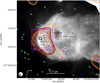 |
Fig. 1 Observations of IC 1396A. Grayscale background image: Herschel/PACS 70 μm. Orange contours: NIKA 1.3 mm data (15 contours, starting at 3σ = 0.007 Jy beam−1 up to 0.3 Jy beam−1 in log scale). Brown contours: NIKA 2 mm data (15 contours, starting at 3σ = 0.003 Jy beam−1 up to 0.14 Jybeam−1 in log scale). The rms increases toward the edges of the field. The field observed with EMIR is marked with a pink dashed box. Known young objects are marked as green stars (detected in the optical; Sicilia-Aguilar et al. 2004, 2005a, 2013; Barentsen et al. 2011), magenta stars (detected in the IR; Reach et al. 2004; Sicilia-Aguilar et al. 2006a; Morales-Calderón et al. 2009), and blue inverted triangles (X-ray detections; Getman et al. 2012). The Class 0 source, marked with a black square, is located in the coolest and densest part of the globule. V 390 Cep is marked with a red circle. The protostar α (Reach et al. 2004) is also labeled. The beams for 1.3, 2, and 3 mm are shown in the lower left corner. |
Summary of the molecular line observations.
Strong lines detected in the high-resolution spectra.
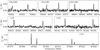 |
Fig. 2 Some of the complex molecules and carbon chain lines detected toward the region. Top panel: CH3 CHO. Middle panel: C4H. Bottom panel: C2H. |
2.2. Ancillary data
A wealth of existing optical and IR data were used to obtain a complete (multiphase, dust and gas, and temperature range from stellar photospheres to tens of K) view of the globule and its embedded population. Our Herschel/PACS data at 70 and 160 μm6 (for further details regarding observations and data reduction, see Sicilia-Aguilar et al. 2015, Paper I) are particularly useful for the characterization of the dust content in the globule and of IC 1396A-PACS-1. Our [S II] narrow-band imaging, obtained with CAFOS on the 2.2 m telescope in Calar Alto (Sicilia-Aguilar et al. 2013) allows us to characterize the edge of the PDR and the impact of the embedded population in the cloud. Finally, Spitzer IRAC and MIPS data (Reach et al. 2004; Sicilia-Aguilar et al. 2006a; Morales-Calderón et al. 2009), together with optical high-resolution spectroscopy (Sicilia-Aguilar et al. 2006b), complete the characterization of the low-mass cluster members in the region and the radial-velocity picture obtained from the molecular lines, respectively.
In addition, we used Gaia DR2 data (Gaia Collaboration 2016, 2018a) that are available through Vizier (Gaia Collaboration 2018b) to explore the velocities of the stars that are associated with IC 1396A and the Tr 37 cluster in connection with the molecular gas observations. Gaia has been successfully used to identify the cluster structure in other young clusters (e.g., Roccatagliata et al. 2018; Franciosini et al. 2018), and can help to obtain a three-dimensional picture of the region. We compiled the list of cluster members in Tr 37 and the IC 1396A region based on spectroscopically identified members (Contreras et al. 2002; Sicilia-Aguilar et al. 2005a, 2006b, 2013), Spitzer identifications (Reach et al. 2004; Sicilia-Aguilar et al. 2006a; Morales-Calderón et al. 2009), Hα photometry (Barentsen et al. 2011), and X-ray surveys (Mercer et al. 2009; Getman et al. 2012). This produced a list of over 800 members detected with Gaia, 354 of which had low errors (matching radius <0.5 arcsec, relative parallax error σω /ω < 0.1, and proper motion errors below 2 mas yr−1). Of these, 6 sources are associated with IC 1396A, including V390 Cep, which is known to be physically associated with the globule through the signs of interaction within the eye-shaped hole. A histogram with the Gaia parallaxes for Tr 37 and IC 1396A is shown in Fig. 3.
For a cluster at a relatively large distance that is composed of mostly low-mass, faint stars, the errors from Gaia DR2 are often non-negligible, which results in biased distances if the parallaxes are simply inverted. Because of this, we followed the Bayesian inference methods of Bailer-Jones (2015) and Astraatmadja & Bailer-Jones (2016a,b) to estimate distances and their asymmetric errors. The distance to the cluster members was obtained by assuming an exponentially decreasing density prior, which is the preferred one for DR2 (Bailer-Jones et al. 2018), with a characteristic length l = 1.35 kpc (Astraatmadja & Bailer-Jones 2016a,b). Following Bailer-Jones (2015), the prior for an exponentially decreasing density can be written as a function of the distance r and the characteristic length l,
 (1)
(1)
For this, the unnormalized posterior is a function of the parallax ω and the parallax error σω
![Mathematical equation: \begin{equation*} P^*_{r^2 e^{-r}}(r | \omega, \sigma_{\omega})=\begin{cases} \frac{r^2 e^{-r/l}}{\sigma_{\omega}} \textrm{exp}[-(\omega-1/r)^2/2\sigma^2_{\omega}] &\text{if $r>0$},\\ 0 & \text{otherwise}. \end{cases} \end{equation*}](/articles/aa/full_html/2019/02/aa33207-18/aa33207-18-eq2.png) (2)
(2)
The best estimate of the distance was calculated as the mode of the unnormalized posterior, which can be obtained from equating the derivative of the posterior to zero (Bailer-Jones 2015). Using the 354 stars with good Gaia data, we find that the average distance to the cluster is found to be 945 pc, where the error bars mark the 5–95% confidence intervals. This is consistent with the previous value of 870 pc (Contreras et al. 2002), especially as we take into account that Gaia DR2 seems to be slightly biased toward larger distances (Stassun & Torres 2018), which will be corrected in future data releases. The stars associated with IC 1396A are consistent with the cluster distance, as expected from the evident physical relation between the globule and HD 206267 (see Fig. 3 left).
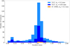 |
Fig. 3 Histogram of the parallaxes of the known Tr 37 cluster members with good Gaia data (see text). The stars associated with IC 1396A are plotted in yellow. |
3. Data analysis
3.1. Dust temperature and column density maps
Although optical and Spitzer images suggest a relatively uniform globule with a hole around the position of V 390 Cep, Herschel unveiled denser, colder material behind the ionization front (Paper I). The NIKA data confirm the Herschel results, showing a sharp rise inintensity behind the ionization rim, with an intensity varying by over a factor of 40 at both 1.3 and 2 mm between the maximum point at the Class 0 source and the lower density structures to the west (see Fig. 1).
The temperature and column density map from Herschel data alone (Sicilia-Aguilar et al. 2015) is highly uncertain because only two wavelengths were used. Here, we revise the SED of the Class 0 object, together with the dust temperature and column density maps around IC 1396A-PACS-1 using the NIKA data in combination with Herschel/PACS. For the object SED, we combined the Herschel data (see Paper I) with the integrated NIKA flux at the position of the Class 0 source. We defined the source limits based on the background emission around the extended structure, which is 0.09 and 0.04 Jy beam−1 at 1.3 and 2 mm, respectively. The errors in the NIKA fluxes depend not only on the calibration and filtering uncertainties (see Sect. 2.1), but also on the uncertainties that define the source limits in a region with highly variable background, for which we adopted a conservative estimate of ~30%. The SED isdisplayed in Fig. 4. Assuming that the dust is optically thin and that the emission is dominated by a single temperature, the flux emission at a given frequency ν can be written as
 (3)
(3)
Here, kν is the mass absorption coefficient, Ω is the solid angle subtended by the emitting region, Σ is the mass column density, and Bν(T) is the blackbody emission for a temperature T at the frequency ν. The frequency dependence can be further simplified assuming that the dust mass absorption coefficient kν varies as a power law with frequency, with values that are typically around 2 (e.g., Schneider et al. 2010; Juvela et al. 2012; Preibisch et al. 2012; Roccatagliata et al. 2013). Such a power law also offers a good fit to more detailed dust models in the far-IR and millimeter range (Ossenkopf & Henning 1994).
Although the large NIKA beam includes part of the extended structures detected with Herschel 70 μm data, and thus the interpretation of the emission needs to be regarded with care, the NIKA data confirm that the source is dominated by graybody-like emission, as had been suggested by Herschel. The best-fitting temperatures are in the range of 15–17 K and thus do not significantly change with respect to our previous results based on the two Herschel data points (Paper I). We now take advantage of the NIKA data to derive further constraints on the dust model. The zero-point of this power-law fit depends on the dust properties, including grain sizes, composition, and the presence of icy mantles (Ossenkopf & Henning 1994), all of which are likely to vary throughout a molecular cloud, especially in the surroundings of young objects.
Figure 4 shows the effect of modifying the dust mass absorption coefficients at 70 μm and the power-law exponent of the frequency dependence of the dust mass absorption coefficient, β. Although the typical gas densities in the cloud are expected to be lower (see Sect. 4.2) than those required for substantial dust coagulation (Ossenkopf & Henning 1994), the densities are likely much higher in the source, and dust coagulation and thick ice mantles are a possibility. The temperature is relatively well constrained regardless of the dust model that is used, even though the data suggest a range of temperatures between ~15–17 K in the source. A larger dust mass absorption coefficient would result in lower column densities and lower source masses, even though the value for grains with thin ice mantles of k70 = 118 cm2 g−1 (derived from model 1.b in Table 1 in Ossenkopf & Henning 1994) provides a very good fit to the data. The choice of a larger k70 = 505 cm2g−1 for a model with thick ice mantles (derived from model 1.c in Table 1 in Ossenkopf & Henning 1994) does not appear to be justified by the data. A lower value of β down to 1.7–1.5, as would be expected from grain growth, offers a better fit, even though it is very hard to distinguish a lower β from the effect of a slight variation of temperature along the line of sight of some degrees (as has been noted in other regions, e.g., Juvela & Ysard 2012).
The best-fitting mass column density Σ from Eq. (3) can be used to derive a mass for the envelope of the Class 0 object. Assuming a gas-to-dust ratio (Rgas/dust = 100) and take into account the mass of the hydrogen atom (mH) and the mean molecular weight (μ = 2.8), the hydrogen number column density (NH) can be estimated as
 (4)
(4)
which can be integrated over the size of the object to derive a total mass. The limits of the source are uncertain, with the object appearing as a compact source at 70 μm and the envelope being resolved at 160 μm (Paper I). Assuming a size similar to the NIKA 1 mm beam, we obtain a mass in the range of 7–18 M⊙ for typical models with k70 = 118 cm2 g−1 and β = 1.5–1.9. Given that the lower masses result from the fits that better adjust to the Herschel and that the source is likely optically thick at 70 μm, higher masses are likely more representative of the Class 0 envelope mass. The NIKA 2 mm datum probably contains part of the cloud emission, since the source envelope is resolved at 160 μm and appears smaller than the NIKA 2 mm beam. A larger dust mass absorption coefficient would result in a lower mass of the source, and extending the source limits to the NIKA 2 mm beam would result in a mass that would be higher by a factor of 2.
To derive the temperature and column density maps, we extended the assumption of single dust temperature and optically thin material to the whole cloud (see Roccatagliata et al. 2013, for further details on this approximation). The first assumption breaks down if the cloud has a temperature structure along the line of sight, which is usually expected. In regions with different temperatures, the emission is dominated by the highest temperature on the line of sight. If emission from a hot point-source (such as a star or protostar) is significant, then the temperaturewill also be biased toward higher values. In our case, the only protostars with significant emission at 70 μm (compared to the background) in the region are IC 1396A-PACS-1 itself and 21364660 + 5729384 (also called α and located beyond our EMIR field; Reach et al. 2004; Sicilia-Aguilar et al. 2014). The assumption of optically thin material may break down for the 70 μm emission in the very dense parts of the cloud, in particular, around IC 1396A-PACS-1.
The dust column density and temperature structure can be derived by fitting the multiwavelength continuum data point by point using Eq. (3) to obtain a mass column density, Σ, and temperature, and Eq. (4) to derive the hydrogen number column density. For this exercise, we took β = 1.9 (the typical choice for star-forming clouds, Roccatagliata et al. 2013; Sicilia-Aguilar et al. 2015), and for comparison, β = 1.7. We regridded the NIKA and Herschel/PACS maps to the same pixel size (3′′ × 3′′, corresponding to the sampling of our 160 μm PACS maps) and fitted Eq. (3) on a pixel-by-pixel basis to obtain the local temperature and column density. Since the spatial resolution of the 70 μm Herschel data is significantly higher than that of the IRAM data, spatial structures at scales smaller than the IRAM beam are not significant. The pixel-to-pixel variations provide information on the uncertainties of the procedure. For each choice of β, we constructed three separate maps: one including all four Herschel and NIKA bands, a second one including only the 160 μm PACS band and the two NIKA channels, and a third one including both Herschel/PACS bands plus NIKA 1.3 mm channel. The first has the main limitation that the 70 μm band has substantial emission from the Class 0 point source itself, which breaks down the assumption of optically thin material on the source location. The second choice is better suited to characterizing the column density and temperature in the densest parts of the cloud (around IC 1396A-PACS-1), while the third map offers a better view of the extended, less dense cloud (see Fig. 5).
A further limitation of the maps is that because of the filtering that is applied to NIKA data, we underestimate the emission from the low-density parts of the cloud. This results in lower emission coming from regions with extended emission, which would bias the results toward higher temperatures (and lower densities) along the line of sight. To estimate what these losses mean in terms of mass and column density, we can use the differences observed between the three maps described above together with the limits in column density detected in our maps, which can be compared to the column density limits observed with Herschel data only in the region (Paper I, Sicilia-Aguilar et al. 2015). The lowest background column density detected is on the order of 1 × 1021 cm−2 for maps including Herschel data (which is similar to what would be expected for extinction along the line of sight for a region at ~900 pc). Integrating this over the area of the globule, we obtain ~10 M⊙ of low-density material that could be missing in the whole globule. In addition, the globule tail has no significant NIKA emission, and is therefore not included in our mass estimate. Further discussion of this aspect is presented in Sect. 3.2 for the gas-inferred masses.
Despite these uncertainties, the relative values along the line of sight are significant. The temperature and column density maps confirm that the Class 0 source is located in the coldest and densest part of the globule. The NIKA data trace the coldest and densest material more accurately than our previous PACS-only maps (Paper I). In particular, the lack of (proto-)stellar emission and emission associated with the rim behind the photoionization front in the NIKA data compared to PACS allows us to obtain a more accurate picture of the cold envelope around IC 1396A-PACS-1. NIKA also confirms the presence of a low-temperature but lower density region south of PACS-1 (from now on, NIKA S, see Fig. 5), where we do not detect any evidence of ongoing star formation.
The peak of the hydrogen column density at the Class 0 source position is in the range 0.5–10 × 1023 cm−2 for a temperature 14–18 K (depending on the wavelengths used to derive NH 7). Even in the relatively dense NIKA S clump, the densities drop by a factor of 2–6, and the temperatures are about 2–3 degrees higher than around IC 1396A-PACS-1. The differences in density are more marked in the maps that are based on long-wavelength data. Beyond these dense areas, the densities drop to 1–9 × 1021 cm−2 in the parts of the globule that still have some millimeter emission, and below 3 × 1020 cm−2 in the parts with Herschel emission only (Sicilia-Aguilar et al. 2015).
By integrating the column density maps pixel by pixel, we can estimate the total mass in different parts of the globule, keeping in mind that because of the optimization for source extraction in the NIKA maps, the dust emission with low column density may be slightly underestimated. The differences between the maps including NIKA and both (or only one) of the PACS images allow us to estimate the errors in a more accurate way. The total mass in IC 1396A within regions with column densities higher than our 1 × 1021 cm−2 threshold varies depending on the model used and on whether we give more or less weight to the longer or shorter wavelengths. As in Fig. 4, models that include the shorter wavelengths tend to have higher temperatures and thus lower masses than models that include the longer wavelengths. A shallower β = 1.7 tends to produce masses that are nearly a factor of 2 lower than the masses derived with β = 1.9, although lower β values may be hard to justify in the less-dense parts of the globule.
Depending on the choice of parameters and datasets, the total mass of the globule can vary by nearly an order of magnitude between 35 and 270 M⊙. A higher value is more consistent with the complete gas maps obtained for the region (Patel et al. 1995), although wedid not include the whole globule tail. Because the extinction toward the Tr37 cluster is AV = 1.67 mag, with atypical variance between objects of around 0.5 mag (attributed to thin cloud material all around the region plus extinction from circumstellar material; Sicilia-Aguilar et al. 2005a), there is likely a substantial mass of low-density material that is not detected in our maps. The mass in the denser 28′′ region around IC 1396A-PACS-1 ranges between 8 and 80 M⊙, but with themost accurate mass derived from SED fitting, higher masses are favored. For comparison, the NIKA S clump contains between 1–16 M⊙ (with the large range here motivated by the fact that the limits of the clump are poorly defined in flux or temperature and column density), which is only a small fraction of the mass surrounding the Class 0 source. Therefore, regardless of the dust model that is assumed, the head of IC 1396A that contains the Class 0 source also contains about one quarter of the total mass of the globule and is significantly denser than the rest of the structure. We also note that the largest difference inmass, temperature, and column density is not due to small variations in the dust model adopted, but rather on whether the map is more or less strongly weighted toward the shorter or longer wavelengths, with the Herschel-based maps giving higher temperatures and substantially lower masses. To improve these results, a multitemperature fit with additional far-IR and submillimeter data is required, which is beyond the scope of this work.
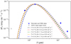 |
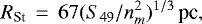
Fig. 4 SED of the Class 0 source including the Herschel and NIKA detections and the MIPS 24 μm upper limit (non-detection) compared to the emission of several modified blackbodies with temperatures 15 and 17 K, β = 1.9, 1.7, and 1.5, and k70 = 118 and 505 cm2g−1 (see discussion in text). Error bars are smaller than the dots for the Herschel data. |
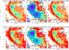 |
Fig. 5 Temperature (color scale) and NH (contours) in the IC 1396A region, derived from all four datapoints (Herschel 70 and 160 μm and the NIKA data; left panels), the Herschel 160 μm and the NIKA data (middle panels), and the Herschel 70 and 160 μm and the NIKA 1.3 mm data (right panels), using a dust model with k70 = 118 cm2 g−1, β = 1.9 (top panels), and k70 = 118 cm2 g−1, β = 1.7 (bottom panels). The 70 μm position of the Class 0 source is marked with a black square, and NIKA S is marked with a triangle. The beams of the two NIKA bands are shown, together with a size indicator. The temperature scales are adapted in each case to show the full range of temperatures with as much detail as possible. Note that there are some biases toward lower or higher temperatures depending on the wavelengths used, as described in the text; relative values are more accurate. The long-wavelength fit is better at determining the global cloud temperature and structure, while the result from the inclusion of the 70 μm temperature is biased toward point-like stellar contributions especially near intermediate-mass protostars such as the objects north of V 390 Cep and the protostar α. The temperature and column density are derived only in the pixels with emission higher than 3σ over the background at all wavelengths. The column density contours mark the 5e21,1e22,5e22,1e23 cm−2 levels, noting that the NIKA + Herschel 160 μm maps start at 1e22 only as they are noise-dominated below this threshold. |
3.2. Gas temperatures and column densities
For the lines that are narrow and strong enough and span a range of upper level energies (Eup) that is wide enough, we estimated the temperatures and densities with a rotational diagram. Given the complexity of the region, we concentrate at this stage on narrow lines that are observed toward the map center, which is dominated by a single component, because complex lines (such as the HCO transitions and the broad CN lines) would need to first be decomposed into their various velocity and density contributors to obtain a meaningful fit. The complete chemical analysis, including the various velocity components, will be presented in a second paper. The main limitation for this exercise is that the lines are weak and the beam is too large for us to be able to distinguish the spatial distribution of the line emission, therefore some of the lines we explored might in part be related to emission from the PDR and in part to the Class 0 source, as is observed for the strongest c-C3H2 line, for instance. Future interferometric data are required for a more detailed picture.
We usedthe CASSIS software8 to extract all the lines in the spectra, fitting a baseline plus Gaussian model to every individual line for a given molecule, examining the fits and the lines for any inconsistent velocities that might represent a line misidentification. For the rotational diagram fit, we assumed an uncertainty of 15% in the flux calibration. The HCOOH lines have large errors and lead to no meaningful excitation temperature, which suggests that some of the transitions are either misclassified, contaminated by other species, or that the emission originates in different regions with various temperatures. The transitions of c-C3H2, CH3CHO, CH3CN,CH3OH, and CCS produce good rotational diagrams and reveal the temperature structure of the gas in the region, although the fit for the CH3OH line has a very large uncertainty. A total of four transitions identified as C4 H produce poor fits regarding velocity and/or S/N, but excluding them results in eight well fit lines for the rotational diagram. An opacity correction to the fits does not significantly change the results, since the errors are dominated by the S/N of the lines. Table 3 summarizes the results, which are displayed in Fig. 6.
The rotational diagrams reveal gas temperatures and column densities that are consistent with the dust observations, assuming typical abundances in star-forming regions. Considering that all the lines are strongest toward the Class 0 source, we can compare the observed temperatures and column densities with those derived for the dust in Sect. 3.1. The density peak around IC 1396A-PACS-1 has a column density of 2 × 10²²–1 × 1024 cm−2 and a temperature around 15–17 K (depending on the wavelengths used to derive the maps). The excitation temperatures of c-C3H2, CCS, and CH3OH are significantly lower than the dominant temperature, which can be due to the fact that the temperature derived from the continuum images is dominated by the highest temperature along the line of sight. CH3CN and CH3CHO track material at a higher temperature than the rest, consistent with observations of WCCC. For CH3OH we find a column density on the order of 1 × 1014 cm−2, which, compared to the hydrogen column density of 2 × 10²²–1 × 1024 cm−2, suggests a ratio CH3OH/H2 = 1 × 10⁻⁸–1 × 10⁻¹⁰, in line with values found in envelopes of cold cores in an early evolutionary stage (van der Tak et al. 2000; Kristensen et al. 2010; Öberg et al. 2014). The higher temperature of CH3CN is consistent with an origin in a deeper and warmer region of the core (Öberg et al. 2014), although the relative abundance with respect to CH3OH (~0.02) is lower than expected, which may be due to beam dilution. CCS is usually found in early-stage star formation and would suggest an age <105 yr for IC 1396A-PACS-1 (Suzuki et al. 1992; de Gregorio-Monsalvo et al. 2006), placing it among the youngest known young stellar objects (YSOs). The abundance of c-C3H2 is similar to what is found in other low-mass star-forming regions, although the low temperature is in contrast with the usual origin of the molecule in the WCCC region (Sakai et al. 2010). Some contamination from c-C3H2 from the PDR region is expected because of the large beam and because some c-C3H2 emission is detected toward the densest parts of the PDR as well (see Sect. 3.3), which may also be the reason for the discrepant temperature values.
A further constraint on the gas mass can be obtained from the integrated line intensity for optically thin lines (Scoville et al. 1986). Our main limitation is the lack of a reliable measure of the excitation temperature since we did not observe several transitions for the same molecule. We followed the procedure in Pineda et al. (2010) to estimate the excitation temperature from the optically thick CO line9. We used their relation between the corrected main-beam temperature (Tmb,c) and the excitation temperature (Tex),
![Mathematical equation: \begin{equation*} T_{\textrm{mb,c}}= T_0 \Big[ \frac{1}{e^{T_0/T_{\textrm{ex}}}-1} - \frac{1}{e^{T_0/T_{\textrm{bg}}}-1} \Big] (1-e^{-\tau}),\vspace*{-3pt}\end{equation*}](/articles/aa/full_html/2019/02/aa33207-18/aa33207-18-eq6.png) (5)
(5)
where T0 = hν∕k for the line frequency, Tbg = 2.73 K is the background temperature, and τ is the line opacity. The main-beam temperatureis related to T by the telescope efficiencies, which gives a factor of 1.559 for the CO(2–1) frequency and 1.522 for the C18O(2–1) transition (Kramer et al. 2013). For a source that is large enough (which may be applied to CO since it is extended rather uniformly over the whole field), the beam filling factor can be taken to ~1. Since CO is optically thick, we can derive its excitation temperature from the line peak, obtaining 39.8 K on the Class 0 source, for which T
 = 22 K for the CO(2–1) line. For comparison, the value for the globule average is 36.6 K (T
 = 20 K), and for the NIKA S clump (T
 = 18 K), we find 33.5 K. Assuming the same excitation temperature for all the CO lines, we can use Eq. (5) to derive the optical depth of the 13CO and C18O lines.
We find that τ13CO ~1 in all regions, which means that it is marginally optically thick. For C18O, the assumption that the emission comes from a region that is far larger than the beam breaks down. While it is true that the emission is strongly peaked at the position of the Class 0 source, there is some significant emission toward NIKA S and all around the globule. We thus estimate a filling factor of 0.7 for the compact sources (assuming a size comparable to the NIKA 2 mm beam for the C18O emission, see, e.g., Shimajiri et al. 2014). This gives us τC18O = 0.31 in the Class 0 source, and τC18O = 0.16 in the NIKA S clump. With these values, the C18O column density (NC18O) can be derived (see, e.g., Scoville et al. 1986; Ao et al. 2004; Pineda et al. 2010). Assuming that the excitation temperature is much higher than the background temperature and using the beam-averaged opacity τ, we obtain
 (6)
(6)
where h and k are the Planck and Boltzmann constants, respectively, J is the quantum number of the lower level, B is the rotational constant (54.891 GHz for C18O10), and μ is the electric dipole moment (0.1098 Debye for C18O).
To calculate the mass of the sources, we need to take the abundance of C18O with respect to H2 into account. There is a substantial uncertainty in this, which moreover depends on the type of region observed (e.g., PDR regions vs. YSO vs. HII regions), with some authors suggesting lower (Areal et al. 2018) or higher (Shimajiri et al. 2014) C18O versus H2 abundances that can lead to significantly different results. We adopted the calibration of Frerking et al. (1982) for high-density enviroments in ρ Ophiuchus. The resulting H2 column densities range from 8.5e + 23 cm−2 in the Class 0 source to 4.1e + 23 cm−2 in NIKA S, and 7e + 22 cm−2 for the globule average within the EMIR map. These values are roughly comparable to the values derived from the 160μ plus NIKA 1 mm, 2 mm column density map, and as in this case, more weighted toward lower temperatures and higher densities. Using the same mean molecular weight 2.8 and taking the size of the sources into account, we estimate a mass for the Class 0 source of about 45 M⊙ and 22 M⊙ for the NIKA S clump, which is roughly consistent with the higher estimates based on dust emission. Given the uncertainties in the C18O abundance, the possibility of some degree of C18O being frozenonto the grains and, to a lesser extent, the uncertainties in the excitation temperature, the above given masses are highly uncertain. The results agree well with the amount of mass expected around a forming intermediate-mass star, however.
Since we did not observe the whole globule with EMIR, it is not possible to derive a full-globule mass. The mass derived from the gas observations toward the mapped globule tip suggests that the total gas mass may be a few times higher than the globule estimate from dust mass. Although the dust-based and the gas-based mass estimates for the Class 0 source agree within a factor of a few for the lower temperature estimate, the gas-derived mass of NIKA S is significantly higher, being about half (instead of about 12–20%) of the mass associated with the Class 0 clump. This may be due to a combination of gas freezing in the colder regions (althoug this is not detected in the maps or in the SMA maps; Patel et al. 2015), filtering of extended emission in the NIKA maps, uncertainties in the C18O/H2 ratio, and variations of the excitation temperature and the C18O/H2 ratio throughout the different parts of the globule.
Results of the rotational diagrams obtained with CASSIS.
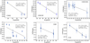 |
Fig. 6 Rotational diagrams showing the best fits to the observed molecular lines. |
3.3. Emission line analysis: exploring the velocity structure of IC 1396A
The global structure of IC 1396A is well characterized by a combination of multi-wavelength, multi-species data. Figure 7 shows a cut through IC 1396A-PACS-1, starting in the outer part cleared by HD 206267, and including the edge of the PDR and along the globule. The Herschel/PACS data clearly show the onset of the dusty globule and the density enhancement where IC 1396A-PACS-1 is located. Narrow-band [S II] data (Sicilia-Aguilar et al. 2013) reveal the peak of the PDR, behind which the dust density rapidly increases. The peak flux of various tracers also reflects their nature, associated with the PDR and/or with the dense globule. The profile across the globule rim and the projected distance between the ionization region (marked by the [S II] peak) and the maximum density (shown by both the Herschel/PACS data and the molecular high-density tracers in Fig. 7) is ~0.09 pc, which is similar to what it would be expected for RDI in a relatively small but massive and dense cloud (Miao et al. 2009) about 0.4 Myr after the onset of significant exposure to ionizing radiation.
A portion of the CN, CS, HCO+, HNC and HCN appears associated with the PDR rim, while highest-density tracers (C18O, N2 D+, DCO+, and SO) peak at the position of the source and the Herschel dust rim, suggesting that the molecular line emission originates from dark regions that are protected from the UV front. The HNC and HCN data can be used as a temperature tracer, since the HNC/HCN ratio is higher than unity in cold regions, and below unity in warmer regions (e.g., Tennekes et al. 2006). Figure 7 shows how the HNC/HCN ratio decreases toward the west of the globule compared to the higher value of HNC/HCN at the source position, revealing a higher temperature toward the less dense parts of the globule, as expected for external heating.
To explore the velocity structure in the region, we first extracted integrated velocity maps of the lines observed with good S/N in the high-velocity resolution mode (see Appendix B). It is not practical to plot the data for individual channels because of the high-velocity resolution of the data and the large number of channels (e.g., over 50 for the 12CO main component and more than 30 for C18O). We therefore present the velocity-integrated line intensity calculated in nine 0.5 km s−1 velocity bins, centered from −9.25 to −5.25 km s−1, which corresponds to the total velocity span observed for all lines. These maps are the first step to visualize and investigate the velocities associated with the different structures within the globule. Based on the velocity maps, on the Herschel data, and on the column density/temperature maps derived from Herschel and NIKA data, we extracted the part of the spectrum corresponding to several distinct structures within IC 1396A, which include the following:
the Class 0 object IC 1396A-PACS-1 (labeled “Class 0” from now on),
the edgeof the PDR region (“PDR”),
the 13CO clump to the southwest of the region (“Clump SW”), which appears globally redshifted,
the arc-shaped structure to the north of the Class 0 object (“Rim N”),
the arc-shaped structure to the south of the Class 0 object (“Rim S”), and
NIKA S, the dense and cold region to the south of the Class 0 object that shows strong NIKA 1 mm emission, as described above.
All the regions were selected to be isolated to avoid contamination by nearby regions, although some contamination is unavoidable because of the beam size. For each region, we estimated the average line emission using GILDAS/Class, which was then used to analyze the velocity structure of the cloud. Figure 8 shows the location of the various components compared to the diverse features in continuum and line emission. These regions appear clearly distinct in their molecular emission (velocity, intensity, and line profile) and also in their general physical properties, although because of projection effects and because of the three-dimensional (3D) structure of the region, we can expect some degree of contamination from other structures in all of them11.
The global structure of the low-density tracers is very complex because the line profiles can include different velocity components along the line of sight even when we integrate over different (projected) spatial locations. The 12CO line is strongly saturated on the globule around the systemic velocity and thus does not offer much information. Nevertheless, the line wings can be used to estimate the limits of the maximum velocities observed in low-density gas along the line of sight, as we discuss in Sect. 4.2. In addition, a faint 12CO component at −0.7 ± 0.1 km s−1 is detected throughout the entire mapped region (see Fig. 10). There is no evidence of gas at this velocity in 13CO or any otherof the tracers, which is a signature of low density and of the line being optically thin. The intensity of the faint 12CO component is quite uniform, increasing toward the west of the region. Its line wings extend up to ±2 km s−1, which is more than is observed in other optically thin lines.
Higher density tracers reveal the density enhancement inside the globule, and even the asymmetry between the less dense northern part and the denser southern side of IC 1396A. When we exclude the lines that are highly saturated and have distorted profiles (12CO and 13CO) and concentrate on lines that are observed toward all five regions (such as C18O, HCO+, and HNC; Fig. 9), we also observe that the line width increases off-source and that the Class 0 object is systematically blueshifted by 0.5–1 km s−1 with respectto the surrounding nebula. The blueshifted asymmetry points toward collapse, while the increased line width is consistent with increased turbulence and the bulk motions in the surrounding clump. The off-source line profiles are also asymmetric but less sharply peaked than on-source. They are blue-dominated and thus suggestive of collapse or, in case of a globule thatis being photoionized on the far side from our line of sight, it could be a sign of generalized RDI. The broad but asymmetric profiles of the lines in the less dense parts of the globule are consistent with the gas being disrupted and removed from the globule by the effect of HD 206267.
Only the region around IC 1396A-PACS-1 has significant emission in high-density tracers (such as DCO+, N2 D+, and H2CO; see Fig. 9). There is weak DCO+ emission associated with Rim S, although it is one order of magnitude weaker than the emission associated with the IC 1396A-PACS-1 core. This indicates that the Class 0 protostar is forming in the densest parts of the globule, and is consistent with the column density that is a factor of 5–10 higher around IC 1396A-PACS-1, measured by the continuum observations. The 13CO line is saturated at the position of the source, while the C18O presents a blue-asymmetric profile. There is no evidence of CO depletion in the source, despite the detection of nitrogenated species and the potential disparity between gas-based and dust-based masses, which could be an effect of the large beam and the complexity of the source to be explored with higher resolution observations (see Patel et al., in prep). The C18O line profile could be interpreted as infall, athough the proximity of the PDR and the photoevaporative velocities associated with it and the fact that the 13CO presents the same blue-dominated profile toward the rest of the cloud suggest that the profile could be also affected by global cloud motions and photoevaporation. The rest of emission lines from high-density tracers, especially for those detected with high S/N (DCO+ and N2 D+), are the best indicators of the properties and velocity of the Class 0 source, and in this case, they are also found to be asymmetric, with a blueshifted peak, which is suggestive of infall in the densest parts of the core.
We also find that the SW clump, in addition to being redshifted, has systematically larger line widths than the rest of the structures. In general, the cloud positions have a significantly stronger extended red tail than the object. Both the Class 0 source and the PDR lack these red tails, which is a further point suggesting the association of IC 1396A-PACS-1 and the ionization front. Detailed inspection of the spectra reveals two components in several of the lines (CN and HCN), centered at approximately −8 and −6 km s−1. The redshifted component could be a sign of photoevaporation in the outer parts of the globule facing the O star, while the blueshifted component would correspond to the material associated with IC 1396A-PACS-1. The presence of a redshifted tail and broader lines within the SW clump suggests a higher range of velocities and turbulence, a signature of mass loss and dispersion along several directions over the line of sight, compared to what is observed toward the Class 0 source and PDR rim. Other relatively massive protostars such as α are too far from this redshifted clump for it to be caused by outflows, and the embedded globule population is mostly composed of late-type Class I and Class II objects that are not expected to drive such powerful and broad outflows as to explain the SW redshifted emission.
The next step was to analyze the pixel-by-pixel structure in the different line tracers for which we have high-resolution data. Since the lines are highly complex and often self-absorbed, we used a multi-Gaussian approach to create a model-independent, non-parametric way of describing the line strength, velocity, and width. Although multi-Gaussian fits have been successfully used on large scales (e.g., Hacar et al. 2013), the environment around IC 1396A-PACS-1 is highly complex and the multi-Gaussian fits are strongly degenerate. Therefore, in an analogy to complex optical emission lines (e.g., Sicilia-Aguilar et al. 2017), we instead derived several line parameters, including line peak and peak velocity, integrated flux, line width, and line asymmetry (blue vs. red components for both the flux and the velocity). As occurs in the optical, molecular emission lines can be extremely complex, and thus a simple geometrical fit does not have a direct physical interpretation, especially in regions where saturation and/or self-absorption occur. The advantage of the fit is that it allowed us to derive line-based parameters that take the global shape of the line into account and thus enabled us to systematically explore emission, velocities, and line asymmetry on a pixel-by-pixel scale. In this way, we can visualize and detect changes of the structure that are not seen by other means such as channel maps, especially in cases where the structure is very complex and the velocity resolution very high.
For this exercise, the lines were first interactively fit with a multi-Gaussian model containing one to three Gaussian components, selected according to the line shape and the χ2 of the fit. This fit was then used to derive the line parameters, including flux, peak velocity, width, and asymmetry in flux and in velocity (seemore details in Appendix C). As long as the Gaussian model profiles provide a good fit (χ2 ≤ 1) to the line, the derived parameters have the advantage that they are not significantly dependent on the particular choice of Gaussian components, so that the line parameters are model independent, circumventing the intrinsic degeneracy of the fit. After this exercise, we can explore the position-velocity, position-width, position-intensity, and position-asymmetry diagrams to derive information about the region. Since the lines originate in gas with different temperatures and densities, the velocities and velocity dispersion in the different gaseous lines give us a 3D dynamical picture of the region, whose details are discussed in Sect. 4.1.
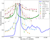 |
Fig. 7 Intensity of various tracers along a cut across the tip of the globule along the line between HD 206267 and IC 1396A-PACS-1. The normalized flux in [S II] and PACS/70 μm data along the same region is also shown. The position of IC 1396A-PACS-1 is marked as a vertical dashed line. HD 206267 would be located at RA = 324.74007, thus at ΔRA = +0.46907° along the same line. The physical scale for a distance of 945 pc is 0.178 pc per ΔRA = 0.02°. |
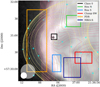 |
Fig. 8 Selected areas in IC 1396A marked by colored boxes. The background gray image with white contours is the Herschel/PACS 70 μm map. The yellow contours show the NIKA 1.3 mm emission as in Fig. 1. The violet contours display the 13CO emission (23 linear contours in the range 8–30 K (T |

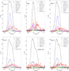 |
Fig. 9 Average emission lines detected toward the various regions delineated in Fig. 8. The line profiles and strength between the Class 0 core and the rest of the regions are significantly different. The Rim S region also appears to be denserthan the rest, although it is clearly less dense than observed toward the Class 0 source. High-density tracers (N2 H+ and DCO+) are only observed toward the densest regions. The CN line (which is presented here multiplied by a factor of 3 because it is relatively weak) is strongly associated with the edges of the cloud, as expected if it is dominated by the photoevaporating cloud interface. |
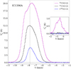 |
Fig. 10 Averaged 12CO and 13CO emission toward IC 1396A. The inset shows the faint component at velocity −0.7 km s−1. There is no detectable 13CO emission at this velocity. |
3.4. Tangential velocities from Gaia DR2
Further information regarding the velocity of the globule can be obtained from the analysis of the Gaia DR2 data (Gaia Collaboration 2016, 2018a). The cluster proper motion can be calculated by the weighted average of the individual proper motions for the 354 objects with good Gaia data (see Sect. 2.2), which is μRA = −2.5 ± 1.5 mas yr−1 and μDec = −4.6 ± 1.3 mas yr−1, respectively.The uncertainties given correspond to the typical spread in proper motion between confirmed cluster members, which are estimated as the standard deviation for the 354 cluster members.
Figure 11 shows that the spread of velocities in the plane of the sky of IC 1396A members are similar to what is observed elsewhere in the Tr 37 custer. The proper motions for the globule star V390 Cep, for which its interaction with the surrounding material offer a clear signature of association with the globule, are μRA = −3.53 ± 0.07 mas yr−1 and μDec = −4.78 ± 0.07 mas yr−1. Five more objects are seen in projection against the globule and have good-quality Gaia DR2 data. Including them together with V390 Cep, we derived the weighted mean proper motions for the globule to be μRA = −3.4 ± 0.5 mas yr−1 and μDec = −4.8 ± 0.5 mas yr−1, where the errors reflect the standard deviation of all sources found toward the globule. These values are essentially identical to the velocity of V390 Cep, and all together suggest a tendency for V390 Cep and the globule to move systematically westward (away from HD 206267, see Fig. 11). The proper motion difference is significant in RA, for which ΔμRA = −0.9 ± 0.1 mas yr−1, while the proper motion difference in the Dec direction is essentially consistent with zero, ΔμDec = −0.2 ± 0.1 mas yr−1. For a distance of 945 pc, this is equivalent to 4 km s−1 westward on the plane of the sky (in RA) and up to 0.9 km s−1 northward (in Dec).
4. Discussion: structure and formation history of IC 1396A and Tr 37
4.1. Gas dynamics in IC 1396A
The pixel-by-pixel line component analysis reveals the velocity structure on the plane of the sky with unprecedented resolution. When we consider the various lines together, we can trace the cloud at different depths around the Class 0 source. Many processes (e.g., velocity fields, infall, outflows, depletion, and self-absorption) can affect the shape of the line and thus the line parameters, which means that a single line parameter is unlikely to provide much information on physical processes or structure. Nevertheless, combining them all gives us a powerful way to explore the velocities and velocity gradients throughout the cloud (using the peak velocity for lines that are symmetric and have no signs of self-absorption), detect relative expansion and contraction in higher-density tracers (which induce shifts in the observed peak velocity and line and flux asymmetries with a dominant blue or red part, respectively), or identify the presence of more than one component (e.g., by checking line peaks vs. peaks of individual Gaussian components and the line width).
The 13CO emission rises sharply at the globule rim and is mostly saturated toward the region around IC 1396A-PACS-1, so that the 13CO line parameters do not tell much about the structure of the cloud. The C18O(2-1) line (see Fig. 12) clearly reveals the location of the density peak behind the cloud rim, showing no signs of CO depletion despite the presence of nitrogenated species, probably because of the large beam. The C18O peak velocity shows a strong gradient toward the SW clump, which shows the 3D structure of the globule. The line width also increases in the same direction, as do the line asymmetry for velocity and flux. This indicates a clear change in the velocity pattern and a distinct behavior, compared to the main part of the globule. The velocity asymmetry, and to a lesser extent, the flux asymmetry, also reveal more symmetric, less turbulent lines toward the densest parts of the region. The tendency to find a blueshifted asymmetry in the lines could be an indication of ongoing RDI collapse. The difference in line asymmetry between the inner and the outer part of the globule (Fig. 12) suggests that the globule is being eroded mostly in the outermost parts. The increased width toward the southwest and the fact that the line peak shifts by about half a km s−1 in this direction also points to higher velocities (probably due to evaporation of the near side of the globule) in this region.
Several PDR-related lines are detected within our EMIR field. This includes a very weak SiO line and CN emission. The SiO line is very weak, but detected toward the PDR, the Class 0 object, and the extended southern rim (Rim S). The CN line is remarkably broad and globally redshifted compared to all other lines. It has a typical central velocity of approximately −6.5 km s−1 and a 10% width in the 3–4 km s−1 range. A global redshift is typically observed in optical lines toward the tips of PDR pillar-like structures (McLeod et al. 2015), which is observed in the multi-Gaussian analysis of the CN line. The central velocities of all other strong lines, which appear around −7.8 km s−1, instead track denser material inside the globule. The structure of the CN line is also quite stable throughout the globule and is usually well fit by two individual Gaussian components, although since the line is weak, there is a substantial uncertainty in the line parameters. The first component peaks at approximately −6.4 km s−1, and the second peaks at approximately −8.1 km s−1. The blueshifted component dominates toward the Class 0 source and the northern side of the PDR rim. It is also the narrowest component (~0.6 km s−1), and its width increases toward the globule rim. The redshifted component is very variable in intensity and line width (~0.9−1.2 km s−1), and it does not show any discernible pattern, except that it is stronger around the PDR region. Both components can be interpreted as the redshifted and blueshifted sides of a photoevaporation flow, where the most distant side of the globule would be more photoevaporated, as expected if the far side receives more illumination by HD 206267. The velocity difference compared to the rest of lines would be about 0.6 km s−1.
The HCN and HNC lines have similar line profiles, with the difference in flux (related to the temperature) pointed out previously. The 3D maps show that HCN is quite uniform over the globule, while HNC is clearly stronger toward the rim, as expected (see Fig. 13 left). Both lines have a slight blue-dominated asymmetry, and their peak velocity does not vary much over the mapped area, but shows a relatively constant offsets of about 0.3−0.4 km s−1 (see Fig. 13 middle). This likely is an optical depth effect. HCN is more blueshifted, with a velocity similar to the blueshifted CN component (which may also indicate a photoevaporation origin), and it tends to be slightly broader than HNC.
The HCO+ line intensity increases steeply toward the globule and also shows a trend to redder velocities in the western part of the globule, which could be a sign of material loss and globule evaporation. The peak is at the rim, as expected for a high-density tracer. Higher density lines such as DCO+ and N2 D+ are detectable only in the densest part of the globule (Fig. 13 right). They have blue-dominated profiles characteristic of infall, and a peak velocity of −7.8 km s−1 (DCO+) and −8.0 km s−1 (N2 D+). The lines are relatively narrow and weak, which makes it difficult to analyze the line parameters in detail.
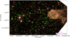 |
Fig. 11 Proper motions of the Tr 37 cluster members between HD 206267 (marked with a large white star) and IC 1396A with parallax errors below 0.2 mas and proper motion errors below 2mas yr−1, shown over the IRAC 1 3.6 μm/Spitzer map of the region. The arrows represent the proper motion with respect to the mean cluster proper motion pmRA = −2.5 ± 1.5 mas yr−1, pmDec = −4.6 ± 1.3 mas yr−1. The stars associated with IC 1396A, including V390 Cep (marked with a blue circle), have proper motions consistent with the cluster, with no evidence of strong acceleration in the plane of the sky. |
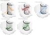 |
Fig. 12 Pixel-by-pixel rendering of the integrated flux, peak velocity, line width, flux asymmetry, and velocity asymmetry (colored dots) for the C18O(2–1) line. The black contours delineate the structures seen in the globule with Herschel/PACS 70 μm. |
 |
Fig. 13 Pixel-by-pixel rendering of the integrated flux (left panel) and peak velocity (middle panel) of the HCN(1–0) (yellow dots) and HNC(1–0) (brown dots) lines, and the integrated flux for the DCO+ (3–2) (yellow dots)and N2H+(3–2) (brown dots) lines (right panel). The black contours mark the structures seen in the globule with Herschel/PACS 70 μm. Only the densest parts of the cloud produce significant emission in the high-density tracers N2 H+ and DCO+. |
4.2. Velocity history of IC 1396A within Tr 37
IC 1396A-PACS-1 lies at the interface between a dense cloud and a PDR, as shown in Fig. 7. Based on existing narrow-band images, IC 1396A is a dark globule (Osterbrock 1989; Barentsen et al. 2011), illuminated by HD 206267 mostly from the east. The [S II] images also reveal that although the rim is significantly bright, the [S II] emission from the globule is not significantly different from what is observed toward the H II region (see Fig. 7 and Sicilia-Aguilar et al. 2013). Combined with the thin rim observed in the Herschel continuum data (Paper I), this suggests that the pair HD 206267 and IC 1396A are at a low angle with respect to the plane of the sky. As mentioned in Sect. 4.1, both the velocity and the line width of the CN line are suggestive of an origin in the photoevaporated material around the edge of the globule. The distance between the globule tip and the massive star must be at least equal to the projected distance of 4.9 pc (considering the revised cluster distance of 945 pc). This distance is significantly larger than typically observed toward other photoevaporated globules (such as the Pillars of Creation, at ~2 pc; McLeod et al. 2015).
The velocities of the clouds around the Tr 37/IC 1396 region are very diverse. Wilson (1953) measured a radial velocity of −7.8 km s−1 for HD 206267. This result was later revised by Stickland (1995), who obtained a (highly uncertain) systemic velocity of around −24.8 km s−1 and signatures of spectroscopic binarity. Velocities derived for the CO molecular line emission of the nebular structures in the whole region by Patel et al. (1995) range between VLSR = +5 to −9 km s−1, with IC 1396A having VLSR = −7.9 km s−1. The velocity we derive for IC 1396A is fully consistent with that value, VLSR = −7.8 km s−1 on average, and with previous estimates of the velocity of the globule (Morgan et al. 2010). Lines with various optical depths show slightly different velocities, which suggests a small variation by ~0.3 km s−1 throughout different depths. In particular, lines associated with the PDR are clearly redshifted compared to high-density tracers. This is consistent with the surface of the cloud being eroded.
The radial velocities of the parental cluster Tr 37 are significantly different from those of IC 1396 by about 7 km s−1. Sicilia-Aguilar et al. (2006b) used optical spectroscopy to measure the radial velocities of T Tauri stars (and their spread) in Tr 37, obtaining a typical radial velocity cz = −15.0 ± 3.6 km s−1 (VLSR ~ −1 km s−1), which is clearly distinct from that of IC 1396A. Molecular-line 12CO emission has been also detected toward a star with a remarkably massive disk (GM Cep; Sicilia-Aguilar et al. 2008), confirming the VLSR = −1 ± 2 km s−1, in agreement with the optical mean velocity of the Tr 37 cluster. The 12CO weak component centered at −0.7 km s−1 (Fig. 10) appears relatively uniform over IC 1396A, which suggests that it corresponds to a diffuse component tracing low-density remnant material of the original cloud that gave rise to Tr 37. Combined with the velocity in the plane of the sky measured with Gaia, we obtain a velocity difference of about 8 km s−1 in magnitude between IC 1396A and Tr 37. This distinct velocity suggest different origins for both the main Tr 37 cluster and IC 1396A within parts of the many clouds that constitute the Cep OB2 region (Patel et al. 1998). With this in mind, the connection between Tr 37 and IC 1396A has to be revised. Exploring the causes of this velocity offset is a first step in this direction. Gravity is unlikely to provide the observed velocity difference. If we consider the approximate mass of the main Tr 37 cluster to be around 1000 M⊙ 12, the velocity expected if IC 1396A were being gravitationally pulled by the main cluster would be on the order of 1 km s−1. Even if we assume a mass higher by 20 times to account for the gas that is now dispersed (for a star formation efficiency of 5%), the gravitational pull would not exceed 4.5 km s−1. This is clearly insufficient to explain the disparate velocities of Tr 37 and IC 1396A. If we consider infall toward the higher mass of the L1149 and L1143 clouds, which are located 50 pc to the east of Tr 37 and have a total mass of 25 200 M⊙ (Patel et al. 1998), the maximum infall velocity expected would only average ~1.5 km s−1.
The natural expansion of H II regions can provide velocity differences between massive star clusters and their surrounding clouds. Considering the expansion of a Strömgren sphere (McKee et al. 1984; Osterbrock 1989), the Strömgren radius RSt is given by
 (7)
(7)
where S49 is the rate of ionizing photons emitted by the star in units of 1049 photons s−1 (~1.5 for an O6.5 star like HD 206267; Sternberg et al. 2003) and nm is the meannumber density of the cloud. For an isothermal sound speed of cs = 10 km s−1, this translates into an expansion time of
 (8)
(8)
For IC 1396A/HD 206267 and a typical number density of 10 cm−3 (Patel et al. 1998), these values correspond to ~16.5 pc in about 1.4 Myr, which is consistent with the ~15 pc ring of bright-rimmed clouds observed around HD 206267 (Patel et al. 1995; Barentsen et al. 2011). Denser environments would result in smaller radii. For instance, for a distance of 2–2.5 pc, a minimum density of 200 cm−3 would be needed to keep the ionization front from propagating inside a globule, which is well below the estimated density in the thickest parts of IC 1396A.
Rocket acceleration (Elmergreen 1976a,b) of the globule by the effect of the radiation from HD 206267 could induce a velocity away from the ionizing source in a globule like IC 1396A. The magnitude of the imparted velocity can be up to several tens of km s−1, as predicted by some models of BRC evolution (Miao et al. 2006, 2009) and observed in other globules (McLeod et al. 2015). The global velocity observed for IC 1396A is much lower than expected for sustained rocket acceleration, although some degree of rocket acceleration cannot be excluded. To acquire this velocity, globules usually need to be at most at a 2–2.5 pc distance from the ionizing star. One problem with strong rocket effect acceleration is that it predicts line-of-sight velocities on opposite sides of the globule tail and body that are comparable to the bulk motion of the globule (Miao et al. 2006, 2009). Such velocity spreads have been observed in photoevaporated globules (McLeod et al. 2015), but they are inconsistent with the small velocity spread observed for IC 1396A in molecular lines. Our EMIR data detect variations up to ~0.3 km s−1 for lines with different optical depths, up to 2 km s−1 between the red and blue peaks of the CN line, and up to ±4 km s−1 for low-density gas according to the line wings of CO (see Sect. 4.1 and Fig. 10), which would suggest that rocket acceleration accounts for up to a few km s−1 at most. In this respect, the simple expansion models for H II regions from Patel et al. (1995) provide velocities that agree better with the current observations, with a rapid acceleration that would quickly stabilize after 1–2 Myr around a value of ~4–6 km s−1 (see Patel et al. 1995). This value is similar to the velocity on the plane of the sky measured with Gaia, but on the lower side for the observed bulk velocity difference of 8 km s−1. The angle between the velocity vector and the plane of the sky is ~60°, pointing to the west and toward the observer.
If the observed velocity is exclusively caused by rocket acceleration with respect to HD 206267, the angle between the observer, HD 206267, and the globule would be about 30°. This would result in a current distance to the star of nearly 10 pc, which is close to the limit at which the O6.5 star can supply enough ionizing radiation to significantly affect the globule (~11 pc for an O6.5 star with an ionizing flux of 1.5 × 1049 photons s−1; Sternberg et al. 2003; Bisbas et al. 2011). The usual requirement of an ionizing photon flux of at least 1 × 10⁹ photons cm−2s−1 (Bisbas et al. 2011; Miao et al. 2009) imposes a minimum angle of about 30° between IC 1396A and the line of sight toward HD 206267 for the massive star to have a significant effect on the globule. If IC 1396A had been moving at a constant rate, the observed velocities would place it at only 1.1 pc from HD 206267 1 Myr ago. For such a close distance, however, the total expected rocket acceleration would instead be on the order of tens of km s−1 (Miao et al. 2006, 2009) instead of the 8 km s−1 that is observed. The ages of HD 206267 and the Tr37 cluster are 3–4 Myr (Sicilia-Aguilar et al. 2005a; Getman et al. 2012), which poses an additional problem to the idea that the globule is being radially accelerated. A very close (1–2 pc) globule near a massive star would be subject to strong acceleration and would lose matter at a rate of at least several tens of solar masses per Myr (McLeod et al. 2016), which would halve the mass of a globule like IC 1396A in about 0.3–0.4 Myr (Miao et al. 2006, 2009) for an ionizing photon flux of ~1.5e11 cm−2 s−1. This value is reached at a distance of about 1 pc from HD 206267. This means that if the velocity is entirely radial, it cannot have been constant in time (scenario 1), or that the velocity we observed cannot be exclusively due to rocket acceleration in the radial direction away from the star (scenario 2).
While the expansion of the H II region is expected to slow down with time, rocket acceleration is expected to increase in time, and the velocity saturates when the HII region is about 10 pc away and ~2 Myr old (Patel et al. 1995). In scenario 1, IC 1396A would currently be at about ~10 pc from the ionizing source (~30° angle with respect to the line of sight toward HD 206267). This distance is comparable to the models for the expansion of an H II region for an age between 2 and 3.5 Myr for Tr 37 (see Fig. 11 in Patel et al. 1995), but the bulk velocity of 8 km s−1 is about a factor of 2 higher than expected. This means that a short time at the observed velocity would bring IC 1396A too close to HD 206267 for the velocity to be so low compared to the predictions of rocket acceleration.
For scenario 2 and with the angle limitation imposed by the current minimum ionizing flux mentioned above, the only possibility would be to have a larger angle so that IC 1396A would be closer to the plane of the sky and thus currently closer to HD 206267. A closer current distance is also required to cause the observed overpressure (Morgan et al. 2004). This would help understanding the Hα and [S II] emission, and would reconcile the velocity in the plane of the sky with the expansion velocities of the H II region. Nevertheless, scenario 2 also requires an extra velocity component in the radial direction with an origin other than rocket acceleration and/or expansion within the H II region.
Although the expansion velocity is not expected to be constant, the H II region expansion velocities change slowly after the first 1–1.5 Myr (see Patel et al. 1995, Fig. 11). For a cluster age between 3–4 Myr, this means that we can consider the velocity constant in the past 1.5–2 Myr, which are the most relevant for the formation of the population associated with IC 1396A since their ages are estimated to be ~1 Myr (Sicilia-Aguilar et al. 2005a; Getman et al. 2012). For each possible angle between the line of sight, HD 206267, and IC 1396A, we can thus calculate the current distance and extrapolate the distances back in time within the last <2 Myr. The minimum distance to the ionizing source, together with the time at which this minimum distance was reached, are also easy to estimate. Figure 14 shows the results.
The distance to the ionizing source is also a critical parameter for estimating the time needed to disrupt the cloud and whether this time allows for substantial star formation, and it depends on the position of the cloud (see Fig. 14, bottom). For example, for the minimum angle of 30° with respectto the line of sight, a minimum distance of 1.1 pc would have been reached some 1.2 Myr ago (consistent with the Class I/II population), but the distance would only have increased since then, reaching values at the present time that are nearly incompatible with the formation of the Class 0 source.
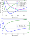 |
Fig. 14 Top panel: distance between IC 1396A and HD 206267 as a function of the current angle with respect to the line of sight (βt=0). Bottom panel: minimum distance between IC 1396A and HD 206267 (blue) and time at which the minimum distance was reached (green) as a function of the current angle with respect to the line of sight (βt=0). The time isgiven in Myr, with the current time set at 0 Myr, which makes all quantities negative. The velocity is considered constant and equal to the velocity observed in the plane of the sky and radial directions, which is a good approximation for the past 2–1.5 Myr (see text). The distances at which the ionizing photon flux is equal to 1e9 and 1e10 cm−2 s−1 are shown as horizontal dotted and dashed lines, respectively. |
4.3. Triggered, sequential, and multi-episode star formation
The revised position and velocity history affects the triggering scenario by affecting the location of the globule with respect to the ionizing source in time. Scenario 1, in which IC 1396A had been initially much closer to the massive star, results in the problem that the observed velocities are only slightly higher than the expansion velocities of the H II region, which is unexpected from rocket acceleration and from what is observed in other BRC (e.g., McLeod et al. 2015). Scenario 1 would also suggest thatthe globule was much closer to the ionizing source 1–2 Myr ago at the time when the most evolved population inside IC 1396A formed (V390 Cep, 14-141, and the Class I/II objects associated with the globule, ~1–2 Myr ago; Reach et al. 2004; Sicilia-Aguilar et al. 2005b, 2006a).
Although IC 1396A is significantly more massive than most of the globules used in RDI simulations, the distance behind the ionization rim at which stars are forming is expected to increase with decreasing ionizing flux (Bisbas et al. 2011). Since the Class 0 source is formed closest to the ionization rim, it is likely that the closest distance between IC 1396A and HD 206267 was reached at about the time of the formation of IC 1396A-PACS-1, thus ≤0.1 Myr. With all associated uncertainties, this suggestsan angle over 70°, which wouldplace the line between IC 1396A and HD 206267 nearly on the plane of the sky. Therefore, if we consider that the Class I population in the globule is farther away from the globule rim than the Class 0 source, we would expect that the globule was located farther away when the 1–2 Myr old population formed. This would result in an angle with respect to the line of sight of at least 37° (assuming an age of 2 Myr for this first population of stars that are now Class II and Class I sources) or 68° (assuming an age of 1 Myr for the first triggered population), which may compromise the possibilities of triggering for the older globule population.
For scenario 2, a velocity component is required that is not related to expansion away from HD 206267. The relatively low observed global velocity can be explained if the globule has in the past been at distances from the ionizing source that are too large to induce any significant acceleration. This is achieved if the current position of the line between HD 206267 and the globule is relatively close to the plane of the sky (<20° with respect to the plane of the sky), which is in agreement with the appearance in Hα and [S II], as mentioned above. Scenario 2 nevertheless introduces the problem that the globule may have been too far away from HD 206267 at the time when the Class I/II population formed for triggered star formation to be efficient. Thus, the options remain that either rocket acceleration and RDI-triggered star formation models are poorly understood or that the only star for which consistent evidence of triggered star formation exists is the Class 0 source IC 1396A-PACS-1.
These dynamical and age considerations make it difficult to confirm the triggering of the oldest populations within the globule. If IC 1396A were located beyond the ϕion = 1e9 cm−2s−1 line about ~1–2 Myr ago, when V390 Cep and 14-141 formed, it would have been beyond the ionization front and too far for RDI (e.g., Bisbas et al. 2011). Figure 14 shows that this is unlikely for 1 Myr at any angle, but it could have been the case for angles lower than about 55° with respect to the line of sight for stars with ages ≥2 Myr old.
Considering that the intermediate-mass star V390 Cep, which belongs to the most evolved globule population, is carving its own ionization hole within the globule without any noticeable external effects, star formation seems to have started relatively unaffected by external influences (either because of a large distance or because it was very highly embedded). The second burst of star formation, resulting in the embedded Class I and Class II sources (Reach et al. 2004; Sicilia-Aguilar et al. 2006a; Getman et al. 2012), appears to be distributed behind the head of the globule, which together with the age difference suggests an RDI-triggering origin (Getman et al. 2012), although the dynamical evidence seems elusive so far. More and deeper observations targeting the lower-density gas and distributed population in the globule could be used to search for further dynamical clues. As the globule approached HD 206267, the ionizing front would have started to erode the less dense parts of the globule, carving it in until it reached the denser core around the Class 0 object IC 1396A-PACS-1. The pressure of the ionization rim now acts directly on the core, as the 70 μm filament shows and as the density, temperature, and turbulence tracers indicate. Therefore, IC 1396A-PACS-1 is the only object in IC 1396A for which an unambiguous sign of triggering exists.
IC 1396A is comparable to the models of 30 M⊙ clouds in the presence of a perpendicular UV radiation field by Kinnear et al. (2014, 2015). The aspect ratio and curvature of the models are very similar to the observed two-arm structure that is detected with Herschel (Paper I) and extends on both sides of the Class 0 source. The collapse time, once exposed to the UV field, would be well below 1 Myr, which is also consistent with the recent formation of the Class 0 source compared to the age of HD 206267 and the Tr 37 cluster. The high mass in the dense core containing IC 1396A-PACS-1 is consistent with the higher-density models in Kinnear et al. (2014), although symmetric clouds tend to produce two cores at the two gravitational foci or ends of the linear structure, which is not the case here. Asymmetries in the direction of the incident UV radiation with respect to the initial dense cloud are also seen in the models if the initial shape of the cloud is elongated along the direction of the incoming UV radiation (Kinnear et al. 2015). The observed differences between the dense core and the rest of the cloud (about 3–4 orders of magnitude in column density) are also consistent with the models, as well as the relatively lower density toward the center of the globule, away from the edges, due to gravitational focusing (Kinnear et al. 2015). The initial density structure of the globule could also contribute to the north-south density difference at the tip of IC 1396A.
4.4. Future evolution of IC 1396A
Considering the current densities and temperatures in the globule, IC 1396A-PACS-1 is also likely to be the last star-forming episode in IC 1396A. Although the NIKA data reveal several smaller clumps in IC 1396A, the temperature maps show that the gas there is significantly warmer, less dense, and contains less mass altogether. Higher resolution observations are required to search for additional star formation, but considering the lack of Herschel counterparts in these regions, it is highly unlikely that more intermediate-mass stars are forming in the globule. Formation of faint, low-mass objects cannot be ruled out at this stage in the denser southern clump and around IC 1396A-PACS-1. IC 1396A-PACS-1 is the predecessor of an intermediate (probably B-type) star (similar to the intermediate-mass star formation inferred in other BRCs, e.g., Morgan et al. 2004). If more low-mass stars were to form within the clump, it could evolve into an irregularly shaped mini-cluster, similar to others observed in other Tr 37, such as those around the binary B star CCDM+5734 (Sicilia-Aguilar et al. 2015).
The NIKA image reveals high-density clumps associated with some of the objects: around the Class II, M1-type, emission line star 21365947+5731349, around the IR source behind 14-141 (at the rim of the V390 Cep hole), on the Class I protostars 21355793+5729099 and 21360798+5726371, surrounding the protostars ϵ and δ, and between the Class I protostar 21364596+5729339 and the K6 Class II object 21364762+5729540 (see reference to the objects in Sicilia-Aguilar et al. 2006a, 2013; Reach et al. 2004). All these objects are Class I and Class II sources without high-mass envelopes, which suggests that the NIKA emission traces extended cloud material and not envelopes. There is a further faint emission to the west of the K6 diskless star 11-2487, although because we lack velocity information, it may correspond to material in the background and not be associated with Tr 37. Although the [S II] forbidden-line map revealed several outflows associated with the low-mass population at the tip of IC 1396A (Sicilia-Aguilar et al. 2013), we do not find any evidence of molecular line emission associated with any of the rest of Class I protostars and T Tauri stars within our EMIR field. This is probably due to a combination of the complexity of the molecular emission from the cloud and PDR, the large beam of IRAM, and the fact that all the objects are of low mass, with low envelope masses and relatively low accretion rates.
The fact that the bulk of the Class I and Class II sources are associated with the less dense material in the globule suggests that a substantial amount of cloud mass has been removed from around the objects. Given that the average ages for objects in the globule is 1 Myr (Sicilia-Aguilar et al. 2006a; Getman et al. 2012), a substantial gas heating and removal needs to have taken place on a relatively short timescale. The connection of the known stars with the warmer parts of the globule may also suggest small-scale feedback, as observed around V390 Cep, but since our temperature estimates are dominated by the highest temperatures along the line of sight, we cannot exclude that far-IR emission from the stars themselves contributes to artificially increase the temperature estimates in their surroundings.
The approximate mass loss due to photoevaporation can be estimated following a method similar to that of McLeod et al. (2015). In their approximation, the total mass loss dM/dt is given by
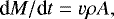 (9)
(9)
where v is the velocity of the photoevaporated gas, ρ is the mass density in the photoevaporating regions, and A is the area of the globule. We consider the velocity of the photoevaporating gas to be on the order of 0.6 km s−1 (from the CN two-component data) and up to ±4 km s−1 for the lowest-density gas with 12CO emission only. The typical column density of the globule in the outermost parts that are subject to photoevaporation can be estimated to be on the order of 7 × 1021 cm−2 (from the NH map), measuring it toward the small, well-defined clump with a radius of 25 arcsec at 21:36:56 +57:31:5813 can be used to estimate an approximate number density ρ = 2 × 104 cm−3. Although the number density of the globule can be significantly higher in the innermost parts, if the photoevaporation is regulated by the photon rate emitted by HD 206267, the rate will not significantly change once the low-density parts of the globule are eroded and denser parts are exposed. Summing over the whole globule area of about 1.5 pc2, we estimate a mass-loss rate on the order of 4 × 10⁻⁴ M⊙ yr−1, which would result in the evaporation of the whole globule on a timescale below 0.5 Myr. This value is on the high end for a globule around a O6.5 star (McLeod et al. 2015), and it is also suggestive of a relatively close distance to the ionizing source at present.
In this calculation, we must note that our dust-derived mass is a factor of 3 lower than previous estimates (Patel et al. 1998), which is probably caused by the fact that our observations are sensitive only to the densest regions. A globule mass of ~100–300 M⊙ is only a few times the mass in stars, based on the stellar census (most of them low-mass stars, see Reach et al. 2004; Sicilia-Aguilar et al. 2006a; Getman et al. 2012). Although some of the sources may be seen in projection, at least half of them show significantly higher extinction and/or are in an earlier evolutionary phase than Tr37, which is suggestive of an association with the globule population. This is an indication that the original globule must have been significantly more massive than it currently is to result in a reasonable star-forming rate, as has been noted by Getman et al. (2012). The fact that substantial mass loss needs to have occurred during the life of the globule is also a sign that despite distance, external photoevaporation must have played an important role in shaping the globule and its population.
From all the above considerations, the environment around IC 1396A-PACS-1 comprises the densest and coldest part of the cloud. Its high density has likely contributed to keep it cold and isolated from previous star formation episodes until the pressure from the expanding H II region was enough to start triggering the collapse. The most massive optically visible star within IC 1396A is V 390 Cep, which is classified as an intermediate-mass star (and thus likely 2–4 M⊙, Contreras et al. 2002; Siess et al. 2000). As an object with A/F spectral type, it produces a very low ionizing flux compared to massive stars, but its action on the cloud is clearly noticeable on small spatial scales, having resulted in the opening of the eye-shaped hole in the globule (see Figs. 1 and 11). The temperature map also reveals local heating and short-scale feedback by the embedded population.
Local feedback in the cloud can be estimated using the A/F-type star V390 Cep as example. With the data on stellar properties and magnitudes (SIMBAD, Wenger et al. 2000), we can estimate its ionizing photon rate to be S ~ 1.5 × 1044 s−1. For this calculation, we assumed the same spectrum as for a white dwarf with the same temperature, and scaled the result to the total stellar luminosity of 2.42 L⊙ (Hills 1973), which gives us S49 ~1.5 × 10⁻⁵ s−1. This flux would result in the opening of a small Stromgren sphere, about 0.15–0.07 pc in radius (depending on the initial cloud density), which agrees well with the observed 0.08 pc size of the hole. The hole is a sign that the local feedback by low-mass stars can be of importance in a cloud with crowded star formation, and its associated gas removal and heating may prevent further star formation on small, nearby scales and significantly contribute to cloud heating and mass loss in the absence of (or far away from) massive stars. The fate of the dense structure along the southern rim and its possibilities of further low-mass star formation may also depend on this small-scale feedback, since the rest of the globule is warmer and significantly less dense.
5. Summary and conclusions
Our NIKA and EMIR data image the IC 1396A globule at millimeter wavelengths with significantly increased resolution compared to previous millimeter studies. We used the dust and gas data to trace the temperature, density, and dynamics of the region, and investigated the origin and triggers of the star formation episodes within the globule. Combining the IRAM data with Gaia DR2 velocities and proper motions, we completed the 3D picture of the region.
Emission suggestive of warm carbon chain chemistry (WCCC) corino is found toward IC 1396A-PACS-1, consistent with the location of the source in an environment with high UV irradiation, although some contamination from PDR lines cannot be excluded at present due to the large IRAM beam. The observed chemistry, and in particular, the presence of CCS associated with the source, place the object among the youngest known protostars. Further interferometric observations are required to confirm the properties and structure of the source.
The head of the globule where IC 1396A-PACS-1 is located appears to be significantly more massive than the rest of the cloud, containing about a quarter of the mass inferred from continuum data, and it is significantly denser and colder than the rest of IC 1396A. From the temperature, density, and dynamical analysis, we conclude that the star formation episode that produced IC 1396A-PACS-1 is probably the last one in IC 1396A, at least regarding intermediate-mass stars, given that the region around the Class 0 object is the last region that appears to be sufficiently dense, cold, and quiescent.
The dynamics of the cloud and its surroundings reveal a new picture of the region. The main velocity of the globule is significantly different from the velocity of Tr 37 (−7.8 vs −1 km s−1), considering both the radial velocities of the stars and of the surrounding gas. We detected a faint 12CO component at −0.7 km s−1, which probably corresponds to the remnants of the cloud that formed Tr 37. The Gaia DR2 stellar proper motions, together with the gas radial velocities, reveal a total velocity of ~8 km s−1 for IC 1396A with respect to Tr 37, which is too low compared to expected rocket acceleration if the globule had been much closer to HD 206267 in the past. Depending on the angle of the globule with respect to the massive star and the line of sight, the distance between IC 1396A and the ionizing source varies, which affects the possibilities of triggering for the older 1–2 Myr population. This result prompted us to revise the history of triggered and sequential star formation in the region, and it also demonstrates the power of combined radial velocity and Gaia data to understand cluster structure and formation history with unprecedented detail.
The formation of V 390 Cep and 14-141 seems to have occurred in a rather undisturbed way. RDI triggering is the most likely formation mechanism for the Class 0 source IC 1396A-PACS-1, and it can be inferred from the blue-dominated profiles of the molecular lines observed toward the source and the globule. The location of the ClassI/II/III population inside IC 1396A is suggestive of RDI (Getman et al. 2012), although the large distance of the globule at the time the stars were formed could have been a problem for triggering.
Finding several star-forming episodes within a structure as small as the IC 1396A globule (~0.5 pc in size) suggests that various modes of sequential fragmentation and star formation can occur in clouds, even on very small spatial scales. The population emerging from such an scenario can thus have age differences of 1–2 Myr, which would also include differences in the evolutionary stage of their disks. Moreover, having various star-forming episodes potentially triggered by different mechanisms may also result in a variety of initial conditions for neighboring protostars, which could lead to potential differences in disk formation and could affect their future evolution.
Acknowledgements
We thank the referee for their thoughtful comments that contributed to clarifying the paper. We also thank the editor, M. Tafalla, for his help during the review process. We are very grateful to the personnel at the IRAM telescope for their help and for making the observation stays so enjoyable. In particular, we are very grateful to M. González, N. Billot, and I. Hermelo for their help with the observation preparation and the observations at the telescope. We also thank Sylvie Cabrit, Ana López-Sepulcre, Nina Sartorio, and Ian Bonnell for their comments and discussion. This work is based on observations carried out under project number 166-13 with the IRAM 30m telescope. IRAM is supported by INSU/CNRS (France), MPG (Germany) and IGN (Spain). This work has made use of data from the European Space Agency (ESA) mission Gaia (https://www.cosmos.esa.int/gaia), processed by the Gaia Data Processing and Analysis Consortium (DPAC, https://www.cosmos.esa.int/web/gaia/dpac/consortium). Funding for the DPAC has been provided by national institutions, in particular the institutions participating in the Gaia Multilateral Agreement. V.R. is partly supported by the European Union’s Horizon 2020 research and innovation programme under the Marie Sklodowska-Curie grant agreement No 664931. This research has made use of the SIMBAD database, operated at CDS, Strasbourg, France. This research was carried out in part at the Jet Propulsion Laboratory, which is operated forNASA by the California Institute of Technology. This research includes analysis carried out with the CASSIS software and the JPL (http://spec.jpl.nasa.gov/) spectroscopic database. CASSIS has been developed by IRAP-UPS/CNRS (http://cassis.irap.omp.eu). This work makes use of the NIST Diatomic Spectral database (https://www.nist.gov/pml/diatomic-spectral-database).This work is partly based on observations obtained with the Herschel Space Telescope within open time proposal “Disk dispersal in Cep OB2”, OT1_asicilia_1. Herschel is an ESA space observatory with scienceinstruments provided by European-led PI consortia and with important participation from NASA.
Appendix A: Line list
The table below contains the entire list of lines detected in the spectra, listed according to their frequency and observed toward the center of the field. For very weak lines, it is not possible to infer the spatial distribution of the emission. The S/N is variable throughout the dataset, especially considering that some of the regions were covered by more than one setup, as listed in Table 1. The presence of multiple carbon chains results in the classification of the source as a potential hot corino.
Lines identified in the low-resolution spectra as observed in the region-averaged spectra.
Appendix B: Velocity-integrated maps for strong lines
Figures B.1–B.6 show the velocity-integrated bit maps for all the strong lines that were observed with the high-resolution configuration. In order to clarify the location of the emitting regions, all maps are shown over the Herschel/PACS 70 μm image. Some of the strong lines show a quadrant structure in some of the momentum maps that is caused by leakage from the strong source. This is stronger toward the edges, where the S/N is lower. The analysis does not include these regions.
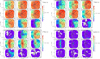 |
Fig. B.1 Velocity integrated bit maps. The colors show the line intensity integrated around 0.5 km s−1 per velocity bin between 3σ and the maximum. White is used when no line emission beyond 3σ is detected in the bin (the bottom of the color scale would usually correspond to the noise level). The velocity bins are much larger than the spectral resolution for the sake of space, as most of the lines are detected in between tens to over two hundred channels. The contours mark for reference the Herschel 70 μm emission on a log scale between 0.1 and 2 Jy beam−1. The beam size is shown for each line. Symbols: IC 1396A-PACS-1 (large black square), other YSO candidates (small black stars). From left to right, top to bottom panels: 12CO, 13CO, C18O, and H2CO. |
 |
Fig. B.5 As Fig. B.1. From left to right, top to bottom panels: HCO, HCO 86.67 GHz, and HCO 86.71 GHz. |
Appendix C: Details on the multi-Gaussian fits and derived line parameters
For the velocity-position analysis, the spectra were first extracted pixel by pixel and then fit using customized interactive Python routines to derive the line properties for each coordinate position. The fit consists of one, two, or three Gaussian components, which can be chosen interactively by the user upon examination of the line and consideration of the χ2 value. In particular, the lines are fit with respect to their velocities using the function f(v),
 (C.1)
(C.1)
where n = 1, 2, or 3, Ai is the amplitude, vi the central velocity, and σi the width ofeach Gaussian component. The fit cannot be directly compared to a physical model, but it is instead used to collect model-free information on how the line profile and intensity varies from pixel to pixel, which can later be interpreted in terms of density, depletion, collapse, or expansion of the gas and to distinguish potential multiple components and multiple velocity structures. Multi-Gaussian fits are usually highly degenerate, especially in the case of low S/N data, therefore we did not use the Gaussian parameters directly, but derived several line properties from them (see Fig. C.1 for a graphical representation), including the velocity of the peak, the line width measured at 10% of the peak height, the flux asymmetry (measured as the ratio of the blue vs. red parts of the observed velocity-integrated flux with respect to the fitted line peak), and velocity asymmetry (measured as the ratio between the line width toward the blue vs. the red parts of the line with respect to the line peak). As long as the fits reproduce the line appropriately (with χ2 ≲1), these properties do not dependent on the individual Gaussians nor on the number of Gaussians used for the fit, which is consistent within the errors. The errors in the individual line parameters are derived from the comparison between the fitted and the observed profiles, taking into account the noise in each particular spectrum. In addition, we also determined the velocity-integrated flux for the whole line by summing the flux in the various observed velocity bins, starting at the 3σ level.
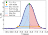 |
Fig. C.1 Line parameters derived from the line fit (dark blue line) for a C18O line, with the data shown as the black step-plot. The peak velocity and flux (Vpeak, Fpeak) are self-explanatory. The line width is measured at 10% of the peak height. The blue and red side of the velocity width are used to determine the blue and red velocity, and the corresponding velocity asymmetry as the ratio of the blue/red velocity. The integrated flux is measured starting at 3σ. The blue and red parts of the flux are ratioed to obtain the flux asymmetry. Although the underlying multi-Gaussian fit is highly degenerate (blue, green, and red dotted lines), the line parameters derived (integrated flux, peak velocity and flux, line width, velocity, and flux asymmetries) will be independent of the fit if the final fit reproduces the line adequately. |
References
- Ao, Y., Yang, J., & Sunada, K. 2004, AJ, 128, 1716 [NASA ADS] [CrossRef] [Google Scholar]
- Areal, M. B., Paron, S., Celis Peña, M., et al. 2018, A&A, 612, A117 [NASA ADS] [CrossRef] [EDP Sciences] [Google Scholar]
- Astraatmadja, T. L., & Bailer-Jones, C. A. L. 2016a, ApJ, 832, 137 [NASA ADS] [CrossRef] [Google Scholar]
- Astraatmadja, T. L., & Bailer-Jones, C. A. L. 2016b, ApJ, 833, 119 [NASA ADS] [CrossRef] [Google Scholar]
- Bailer-Jones, C. A. L. 2015, PASP, 127, 994 [NASA ADS] [CrossRef] [Google Scholar]
- Bailer-Jones, C. A. L., Rybizki, J., Fouesneau, M., Mantelet, G., & Andrae, R. 2018, AJ, 158, 58 [NASA ADS] [CrossRef] [Google Scholar]
- Barentsen, G., Vink, J. S., Drew, J. E., et al. 2011, MNRAS, 415, 103 [NASA ADS] [CrossRef] [Google Scholar]
- Bertoldi 1989, ApJ, 346, 735 [NASA ADS] [CrossRef] [Google Scholar]
- Bisbas, T. G., Wünsch, R., Whitworth, A. P., Hubber, D. A., & Walch, S. 2011, ApJ, 736, 142 [Google Scholar]
- Blitz, L., & Thaddeus, P. 1980, ApJ, 241, 676 [NASA ADS] [CrossRef] [Google Scholar]
- Catalano, A., Calvo, M., Ponthieu, N., et al. 2014, A&A, 569, A9 [NASA ADS] [CrossRef] [EDP Sciences] [Google Scholar]
- Carter, M., Lazareff, B., Maier, D., et al. 2012, A&A, 538, A89 [NASA ADS] [CrossRef] [EDP Sciences] [Google Scholar]
- Caselli, P., & Ceccarelli, C. 2012, A&ARv, 20, 56 [NASA ADS] [CrossRef] [MathSciNet] [Google Scholar]
- Contreras, M. E., Sicilia-Aguilar, A., Muzerolle, J., et al. 2002, AJ, 124, 1585 [NASA ADS] [CrossRef] [Google Scholar]
- Da Rio, N., Tan, J. C., Covey, K. R., et al. 2017, ApJ, 845, 105 [NASA ADS] [CrossRef] [Google Scholar]
- de Gregorio-Monsalvo, I., Gómez, J. F., Suárez, O., et al. 2006, ApJ, 642, 319 [NASA ADS] [CrossRef] [Google Scholar]
- Elmergreen, B. G. 1976a, ApJS, 32, 147 [NASA ADS] [CrossRef] [Google Scholar]
- Elmergreen, B. G. 1976b, ApJ, 205, 405 [NASA ADS] [CrossRef] [Google Scholar]
- Franciosini, E., Sacco, G. G., Jeffries, R. D., et al. 2018, A&A, 616, L12 [NASA ADS] [CrossRef] [EDP Sciences] [Google Scholar]
- Frerking, M. A., Langer, W. D., & Wilson, R. W. 1982, ApJ, 262, 590 [NASA ADS] [CrossRef] [Google Scholar]
- Gaia Collaboration (Prusti, T., et al.) 2016, A&A, 595, A1 [NASA ADS] [CrossRef] [EDP Sciences] [Google Scholar]
- Gaia Collaboration (van Leeuwen, F., et al.) 2017, A&A, 601, A19 [NASA ADS] [CrossRef] [EDP Sciences] [Google Scholar]
- Gaia Collaboration (Brown, A. G. A., et al.) 2018a, A&A, 616, A1 [NASA ADS] [CrossRef] [EDP Sciences] [Google Scholar]
- Gaia Collaboration 2018b, VizieR Online Data Catalog: I/345 [Google Scholar]
- Getman, K. V., Feigelson, E. D., Sicilia-Aguilar, A., et al. 2012, MNRAS, 426, 2917 [NASA ADS] [CrossRef] [Google Scholar]
- Getman, K. V., Feigelson, E. D., Kuhn, M. A., et al. 2014, ApJ, 787, 108 [NASA ADS] [CrossRef] [Google Scholar]
- Hacar, A., Tafalla, M., Kauffmann, J., & Kovács, A. 2013, A&A, 554, A55 [NASA ADS] [CrossRef] [EDP Sciences] [Google Scholar]
- Hernández, J., Calvet, N., Briceño, C., Hartmann, L., & Berlind, P. 2004, AJ, 127, 1682 [NASA ADS] [CrossRef] [Google Scholar]
- Hildebrand, R. H. 1983, QJRAS, 24, 267 [NASA ADS] [Google Scholar]
- Hills, J. G. 1973, A&A, 28, 63 [NASA ADS] [Google Scholar]
- Huang, Y.-F., & Li, J.-Z. 2013, Res. Astron. Astrophys., 13, 557 [NASA ADS] [CrossRef] [Google Scholar]
- Juvela, M., & Ysard, N. 2012, A&A, 539, A71 [NASA ADS] [CrossRef] [EDP Sciences] [Google Scholar]
- Juvela, M., Pelkonen, V.-M., White, G. J., et al. 2012, A&A, 544, A14 [NASA ADS] [CrossRef] [EDP Sciences] [Google Scholar]
- Kinnear, T. M., Miao, J., White, G. J., & Goodwin, S. 2014, MNRAS, 444, 1221 [NASA ADS] [CrossRef] [Google Scholar]
- Kinnear, T. M., Miao, J., White, G. J., Sugitani, K., & Goodwin, S. 2015, MNRAS, 450, 1017 [NASA ADS] [CrossRef] [Google Scholar]
- Kramer, C., Peñalver, J., Greve, A. 2013, IRAM Tech. rep., http://www.iram-institute.org/medias/uploads/eb2013-v8.2.pdf [Google Scholar]
- Kristensen, L. E., van Dishoeck, E. F., van Kempen, T. A., et al. 2010, A&A, 516, A57 [NASA ADS] [CrossRef] [EDP Sciences] [Google Scholar]
- Kuhn, M. A., Feigelson, E. D., Getman, K. V., et al. 2014, ApJ, 787, 107 [Google Scholar]
- Kun, M., & Pasztor, L. 1990, Ap&SS, 174, 13 [NASA ADS] [CrossRef] [Google Scholar]
- Loren, R. B., Peters, W. L., & Vanden Bout, P. A. 1975, ApJ, 195, 75 [NASA ADS] [CrossRef] [Google Scholar]
- Marschall, L. A., & van Altena, W. F. 1987, AJ, 94, 71 [NASA ADS] [CrossRef] [Google Scholar]
- McKee, C. F., van Buren, D., & Lazareff, B. 1984, ApJ, 278, L115 [NASA ADS] [CrossRef] [Google Scholar]
- McLeod, A. F., Dale, J. E., Ginsburg, A., et al. 2015, MNRAS, 450, 1057 [NASA ADS] [CrossRef] [Google Scholar]
- McLeod, A. F., Gritschneder, M., Dale, J. E., et al. 2016, MNRAS, 462, 3537 [NASA ADS] [CrossRef] [Google Scholar]
- Mercer, E. P., Miller, J. M., Calvet, N., et al. 2009, AJ, 138, 7 [NASA ADS] [CrossRef] [Google Scholar]
- Miao, J., White, G. J., Nelson, R., Thompson, M., & Morgan, L. 2006, MNRAS, 369, 143 [NASA ADS] [CrossRef] [Google Scholar]
- Miao, J., White, G. J., Thompson, M. A., & Nelson, R. P. 2009, ApJ, 692, 382 [NASA ADS] [CrossRef] [Google Scholar]
- Mihalas, D. 1978, Stellar Atmospheres (San Francisco: W.H. Freeman and Company) [Google Scholar]
- Monfardini, A., Swenson, L. J., Bideaud, A., et al. 2010, A&A, 521, A29 [NASA ADS] [CrossRef] [EDP Sciences] [Google Scholar]
- Mookerjea, B.,Ossenkopf, V., Ricken, O., et al. 2012, A&A 542, L17 [NASA ADS] [CrossRef] [EDP Sciences] [Google Scholar]
- Morales-Calderón, M., Stauffer, J. R., Rebull, L., et al. 2009, ApJ, 702, 1507 [NASA ADS] [CrossRef] [Google Scholar]
- Morgan, L. K., Thompson, M. A., Urquhart, J. S., White, G. J., & Miao, J. 2004, A&A, 426, 535 [NASA ADS] [CrossRef] [EDP Sciences] [Google Scholar]
- Morgan, L. K., Thompson, M. A., Urquhart, J. S., White, G. J., & Miao, J. 2006, A&A, 457, 207 [NASA ADS] [CrossRef] [EDP Sciences] [Google Scholar]
- Morgan, L. K., Figura, C. C., Urquhart, J. S., & Thompson, M. A. 2010, MNRAS, 408, 157 [NASA ADS] [CrossRef] [Google Scholar]
- Myers, P. C. 1983, ApJ, 270, 105 [NASA ADS] [CrossRef] [Google Scholar]
- Öberg, K. I., Lauck, T., & Graninger, D. 2014, ApJ, 788, 68 [NASA ADS] [CrossRef] [Google Scholar]
- Ossenkopf, V.,& Henning, T. 1994, A&A, 291, 943 [NASA ADS] [Google Scholar]
- Osterbrock, D. E. 1989, Astrophysics of Gaseous Nebulae and Active Galactic Nuclei, (Herndon, VA: University Science Books) [CrossRef] [Google Scholar]
- Padoan, P., & Nordlund, Å. 2011, ApJ, 730, 40 [NASA ADS] [CrossRef] [Google Scholar]
- Patel, N. A., Goldsmith, P. F., Snell, R. L., Hezel, T., & Xie, T. 1995, ApJ, 447, 721 [NASA ADS] [CrossRef] [Google Scholar]
- Patel, N. A., Goldsmith, P. F., Heyer, M. H., & Snell, R.L. 1998, ApJ, 507, 241 [NASA ADS] [CrossRef] [Google Scholar]
- Patel, N. A., Sicilia-Aguilar, A., & Goldsmith, P. 2015, AAS Meeting Abstracts, 225, 211.03 [Google Scholar]
- Peter, D., Feldt, M., Henning, T., & Hormuth, F. 2012, A&A, 538, A74 [NASA ADS] [CrossRef] [EDP Sciences] [Google Scholar]
- Pety, J., Goicoechea, J. R., Hily-Blant, P., Gerin, M., & Teyssier, D. 2007, A&A, 464, L41 [NASA ADS] [CrossRef] [EDP Sciences] [Google Scholar]
- Pickett, H. M., Poynter, R. L., Cohen, E. A., et al. 1998, J. Quant. Spectr. Rad. Transf., 60, 883 [NASA ADS] [CrossRef] [Google Scholar]
- Pineda, J. L., Goldsmith, P. F., Chapman, N., et al. 2010, ApJ, 721, 686 [NASA ADS] [CrossRef] [Google Scholar]
- Preibisch, T., Roccatagliata, V., Gaczkowski, B., et al. 2012, A&A, 541, A132 [NASA ADS] [CrossRef] [EDP Sciences] [Google Scholar]
- Reach, W., Rho, J., Young, E., et al. 2004, ApJS, 154, 385 [NASA ADS] [CrossRef] [Google Scholar]
- Roccatagliata, V., Preibisch, T., Ratzka, T., & Gaczkowski, B. 2013, A&A A6, A554 [Google Scholar]
- Roccatagliata, V., Sacco, G. G., Franciosini, E., & Randich, S. 2018, A&A, 617, L4 [NASA ADS] [CrossRef] [EDP Sciences] [Google Scholar]
- Sakai, N., Sakai, T., Hirota, T., & Yamamoto, S. 2010, ApJ, 722, 1633 [NASA ADS] [CrossRef] [Google Scholar]
- Sandford, M. T., II, Whitaker, R. W., & Klein, R. I. 1980, ApJ 260, 183 [Google Scholar]
- Schneider, N., Motte, F., Bontemps, S., et al. 2010, A&A, 518, L83 [NASA ADS] [CrossRef] [EDP Sciences] [Google Scholar]
- Scoville, N. Z., Sargent, A. I., Sanders, D. B., et al. 1986, ApJ, 303, 416 [NASA ADS] [CrossRef] [Google Scholar]
- Sharpless, S. 1959, ApJS, 4, 257 [Google Scholar]
- Shimajiri, Y., Kitamura, Y., Saito, M., et al. 2014, A&A, 564, A68 [NASA ADS] [CrossRef] [EDP Sciences] [Google Scholar]
- Sicilia-Aguilar, A., Hartmann, L., Briceño, C., Muzerolle, J., & Calvet, N. 2004, AJ 128, 805 [NASA ADS] [CrossRef] [Google Scholar]
- Sicilia-Aguilar, A., Hartmann, L., Szentgyorgyi, A., et al. 2005a, AJ, 129, 363 [NASA ADS] [CrossRef] [Google Scholar]
- Sicilia-Aguilar, A., Hartmann, L. W., Hernández, J., Briceño, C., & Calvet, N. 2005b, AJ, 130, 188 [NASA ADS] [CrossRef] [Google Scholar]
- Sicilia-Aguilar, A., Hartmann, L., Calvet, N., et al. 2006a, ApJ 638, 897 [NASA ADS] [CrossRef] [Google Scholar]
- Sicilia-Aguilar, A., Hartmann, L., Fürész, G., et al. 2006b, AJ 132, 2135 [NASA ADS] [CrossRef] [Google Scholar]
- Sicilia-Aguilar, A., Merín, B., Hormuth, F., et al. 2008, ApJ, 673, 382 [NASA ADS] [CrossRef] [Google Scholar]
- Sicilia-Aguilar, A., Kim, J. S., Sobolev, A., et al. 2013, A&A 559, A29 [NASA ADS] [CrossRef] [EDP Sciences] [Google Scholar]
- Sicilia-Aguilar, A., Roccatagliata, V., Getman, K., et al. 2014, A&A, 562, A131 Paper I [NASA ADS] [CrossRef] [EDP Sciences] [Google Scholar]
- Sicilia-Aguilar, A., Roccatagliata, V., Getman, K., et al. 2015, A&A, 573, A19 [NASA ADS] [CrossRef] [EDP Sciences] [Google Scholar]
- Sicilia-Aguilar, A., Oprandi, A., Froebrich, D., et al. 2017, A&A, 607, A127 [NASA ADS] [CrossRef] [EDP Sciences] [Google Scholar]
- Siess, L., Dufour, E., & Forestini, M. 2000, A&A, 358, 593 [Google Scholar]
- Stassun, K. G., & Torres, G. 2018, ApJ, 862, 61 [NASA ADS] [CrossRef] [Google Scholar]
- Sternberg, A., Hoffmann, T. L., & Pauldrach, A. W. A. 2003, ApJ, 599, 1333 [NASA ADS] [CrossRef] [Google Scholar]
- Stickland, D. J. 1995, The Observatory, 115, 180 [NASA ADS] [Google Scholar]
- Sugitani, K., Fukui, Y., & Ogura, K. 1991, ApJS, 77, 59 [NASA ADS] [CrossRef] [Google Scholar]
- Suzuki, H., Yamamoto, S., Ohishi, M., et al. 1992, ApJ, 392, 551 [NASA ADS] [CrossRef] [Google Scholar]
- Tennekes, P. P., Harju, J., Juvela, M., & Tóth, L. V. 2006, A&A, 456, 1037 [NASA ADS] [CrossRef] [EDP Sciences] [Google Scholar]
- van der Tak, F. F. S., van Dishoeck, E. F., & Caselli, P. 2000, A&A, 361, 327 [NASA ADS] [Google Scholar]
- Watanabe, Y., Sakai, N., Lindberg, J. E., et al. 2012, ApJ, 745, 126 [NASA ADS] [CrossRef] [Google Scholar]
- Wenger, M., Ochsenbein, F., Egret, D., et al. 2000, A&AS, 143, 9 [NASA ADS] [CrossRef] [EDP Sciences] [Google Scholar]
- Wilson, R. E. 1953, General catalogue of stellar radial velocities (Carnegie Institution of Washington Publication) [Google Scholar]
Open Time proposal “Disk dispersal in Cep OB2”, OT1_asicilia_1, PI A. Sicilia-Aguilar, AORs 1342259791 and 1342259792.
Because of the temperature-column density relation, fits based on shorter wavelengths tend to have lower column densities and higher temperatures, which thus leads to lower mass estimates.
This has the strong limitation that the 13CO and C18O lines trace much deeper material than the CO line, therefore their excitation temperatures are likely different.
For instance, the whole region shows PDR-related lines, probably arising from the illuminated globule behind the dark structures we observe in the optical. We also note that the regions with potential leaks across the scan and cross-scan directions are excluded from the analysis (see Appendix B for details).
Based on the known members and considering that the region is essentially devoid of gas now (Sicilia-Aguilar et al. 2006a, 2013; Barentsen et al. 2011).
Choosing other low-density regions does not change the result by more than 30%.
All Tables
Lines identified in the low-resolution spectra as observed in the region-averaged spectra.
All Figures
|
Fig. 1 Observations of IC 1396A. Grayscale background image: Herschel/PACS 70 μm. Orange contours: NIKA 1.3 mm data (15 contours, starting at 3σ = 0.007 Jy beam−1 up to 0.3 Jy beam−1 in log scale). Brown contours: NIKA 2 mm data (15 contours, starting at 3σ = 0.003 Jy beam−1 up to 0.14 Jybeam−1 in log scale). The rms increases toward the edges of the field. The field observed with EMIR is marked with a pink dashed box. Known young objects are marked as green stars (detected in the optical; Sicilia-Aguilar et al. 2004, 2005a, 2013; Barentsen et al. 2011), magenta stars (detected in the IR; Reach et al. 2004; Sicilia-Aguilar et al. 2006a; Morales-Calderón et al. 2009), and blue inverted triangles (X-ray detections; Getman et al. 2012). The Class 0 source, marked with a black square, is located in the coolest and densest part of the globule. V 390 Cep is marked with a red circle. The protostar α (Reach et al. 2004) is also labeled. The beams for 1.3, 2, and 3 mm are shown in the lower left corner. |
| In the text | |
|
Fig. 2 Some of the complex molecules and carbon chain lines detected toward the region. Top panel: CH3 CHO. Middle panel: C4H. Bottom panel: C2H. |
| In the text | |
|
Fig. 3 Histogram of the parallaxes of the known Tr 37 cluster members with good Gaia data (see text). The stars associated with IC 1396A are plotted in yellow. |
| In the text | |
|
Fig. 4 SED of the Class 0 source including the Herschel and NIKA detections and the MIPS 24 μm upper limit (non-detection) compared to the emission of several modified blackbodies with temperatures 15 and 17 K, β = 1.9, 1.7, and 1.5, and k70 = 118 and 505 cm2g−1 (see discussion in text). Error bars are smaller than the dots for the Herschel data. |
| In the text | |
|
Fig. 5 Temperature (color scale) and NH (contours) in the IC 1396A region, derived from all four datapoints (Herschel 70 and 160 μm and the NIKA data; left panels), the Herschel 160 μm and the NIKA data (middle panels), and the Herschel 70 and 160 μm and the NIKA 1.3 mm data (right panels), using a dust model with k70 = 118 cm2 g−1, β = 1.9 (top panels), and k70 = 118 cm2 g−1, β = 1.7 (bottom panels). The 70 μm position of the Class 0 source is marked with a black square, and NIKA S is marked with a triangle. The beams of the two NIKA bands are shown, together with a size indicator. The temperature scales are adapted in each case to show the full range of temperatures with as much detail as possible. Note that there are some biases toward lower or higher temperatures depending on the wavelengths used, as described in the text; relative values are more accurate. The long-wavelength fit is better at determining the global cloud temperature and structure, while the result from the inclusion of the 70 μm temperature is biased toward point-like stellar contributions especially near intermediate-mass protostars such as the objects north of V 390 Cep and the protostar α. The temperature and column density are derived only in the pixels with emission higher than 3σ over the background at all wavelengths. The column density contours mark the 5e21,1e22,5e22,1e23 cm−2 levels, noting that the NIKA + Herschel 160 μm maps start at 1e22 only as they are noise-dominated below this threshold. |
| In the text | |
|
Fig. 6 Rotational diagrams showing the best fits to the observed molecular lines. |
| In the text | |
|
Fig. 7 Intensity of various tracers along a cut across the tip of the globule along the line between HD 206267 and IC 1396A-PACS-1. The normalized flux in [S II] and PACS/70 μm data along the same region is also shown. The position of IC 1396A-PACS-1 is marked as a vertical dashed line. HD 206267 would be located at RA = 324.74007, thus at ΔRA = +0.46907° along the same line. The physical scale for a distance of 945 pc is 0.178 pc per ΔRA = 0.02°. |
| In the text | |
|
Fig. 8 Selected areas in IC 1396A marked by colored boxes. The background gray image with white contours is the Herschel/PACS 70 μm map. The yellow contours show the NIKA 1.3 mm emission as in Fig. 1. The violet contours display the 13CO emission (23 linear contours in the range 8–30 K (T |
| In the text | |
|
Fig. 9 Average emission lines detected toward the various regions delineated in Fig. 8. The line profiles and strength between the Class 0 core and the rest of the regions are significantly different. The Rim S region also appears to be denserthan the rest, although it is clearly less dense than observed toward the Class 0 source. High-density tracers (N2 H+ and DCO+) are only observed toward the densest regions. The CN line (which is presented here multiplied by a factor of 3 because it is relatively weak) is strongly associated with the edges of the cloud, as expected if it is dominated by the photoevaporating cloud interface. |
| In the text | |
|
Fig. 10 Averaged 12CO and 13CO emission toward IC 1396A. The inset shows the faint component at velocity −0.7 km s−1. There is no detectable 13CO emission at this velocity. |
| In the text | |
|
Fig. 11 Proper motions of the Tr 37 cluster members between HD 206267 (marked with a large white star) and IC 1396A with parallax errors below 0.2 mas and proper motion errors below 2mas yr−1, shown over the IRAC 1 3.6 μm/Spitzer map of the region. The arrows represent the proper motion with respect to the mean cluster proper motion pmRA = −2.5 ± 1.5 mas yr−1, pmDec = −4.6 ± 1.3 mas yr−1. The stars associated with IC 1396A, including V390 Cep (marked with a blue circle), have proper motions consistent with the cluster, with no evidence of strong acceleration in the plane of the sky. |
| In the text | |
|
Fig. 12 Pixel-by-pixel rendering of the integrated flux, peak velocity, line width, flux asymmetry, and velocity asymmetry (colored dots) for the C18O(2–1) line. The black contours delineate the structures seen in the globule with Herschel/PACS 70 μm. |
| In the text | |
|
Fig. 13 Pixel-by-pixel rendering of the integrated flux (left panel) and peak velocity (middle panel) of the HCN(1–0) (yellow dots) and HNC(1–0) (brown dots) lines, and the integrated flux for the DCO+ (3–2) (yellow dots)and N2H+(3–2) (brown dots) lines (right panel). The black contours mark the structures seen in the globule with Herschel/PACS 70 μm. Only the densest parts of the cloud produce significant emission in the high-density tracers N2 H+ and DCO+. |
| In the text | |
|
Fig. 14 Top panel: distance between IC 1396A and HD 206267 as a function of the current angle with respect to the line of sight (βt=0). Bottom panel: minimum distance between IC 1396A and HD 206267 (blue) and time at which the minimum distance was reached (green) as a function of the current angle with respect to the line of sight (βt=0). The time isgiven in Myr, with the current time set at 0 Myr, which makes all quantities negative. The velocity is considered constant and equal to the velocity observed in the plane of the sky and radial directions, which is a good approximation for the past 2–1.5 Myr (see text). The distances at which the ionizing photon flux is equal to 1e9 and 1e10 cm−2 s−1 are shown as horizontal dotted and dashed lines, respectively. |
| In the text | |
|
Fig. B.1 Velocity integrated bit maps. The colors show the line intensity integrated around 0.5 km s−1 per velocity bin between 3σ and the maximum. White is used when no line emission beyond 3σ is detected in the bin (the bottom of the color scale would usually correspond to the noise level). The velocity bins are much larger than the spectral resolution for the sake of space, as most of the lines are detected in between tens to over two hundred channels. The contours mark for reference the Herschel 70 μm emission on a log scale between 0.1 and 2 Jy beam−1. The beam size is shown for each line. Symbols: IC 1396A-PACS-1 (large black square), other YSO candidates (small black stars). From left to right, top to bottom panels: 12CO, 13CO, C18O, and H2CO. |
| In the text | |
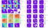 |
Fig. B.2 As Fig. B.1. From left to right, top to bottom panels: N2 H+, N2 D+, HCO+, and DCO+. |
| In the text | |
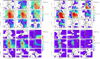 |
Fig. B.3 As Fig. B.1. From left to right, top to bottom panels: C34S, C33 S, 13 CS, and CCS. |
| In the text | |
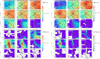 |
Fig. B.4 As Fig. B.1. From left to right, top to bottom panels: HCN, HNC, H13 CN, and HC15N. |
| In the text | |
|
Fig. B.5 As Fig. B.1. From left to right, top to bottom panels: HCO, HCO 86.67 GHz, and HCO 86.71 GHz. |
| In the text | |
 |
Fig. B.6 As Fig. B.1. From left to right, top to bottom panels: SO(2-1), SO(5-4), CN, and c-C3 H2. |
| In the text | |
|
Fig. C.1 Line parameters derived from the line fit (dark blue line) for a C18O line, with the data shown as the black step-plot. The peak velocity and flux (Vpeak, Fpeak) are self-explanatory. The line width is measured at 10% of the peak height. The blue and red side of the velocity width are used to determine the blue and red velocity, and the corresponding velocity asymmetry as the ratio of the blue/red velocity. The integrated flux is measured starting at 3σ. The blue and red parts of the flux are ratioed to obtain the flux asymmetry. Although the underlying multi-Gaussian fit is highly degenerate (blue, green, and red dotted lines), the line parameters derived (integrated flux, peak velocity and flux, line width, velocity, and flux asymmetries) will be independent of the fit if the final fit reproduces the line adequately. |
| In the text | |
Current usage metrics show cumulative count of Article Views (full-text article views including HTML views, PDF and ePub downloads, according to the available data) and Abstracts Views on Vision4Press platform.
Data correspond to usage on the plateform after 2015. The current usage metrics is available 48-96 hours after online publication and is updated daily on week days.
Initial download of the metrics may take a while.