| Issue |
A&A
Volume 621, January 2019
|
|
|---|---|---|
| Article Number | A46 | |
| Number of page(s) | 12 | |
| Section | Extragalactic astronomy | |
| DOI | https://doi.org/10.1051/0004-6361/201834291 | |
| Published online | 03 January 2019 | |
Analyzing temporal variations of AGN emission line profiles in the context of (dusty) cloud structure formation in the broad line region
1
Max Planck Institut für Astronomie, Königstuhl 17, 69117 Heidelberg, Germany
e-mail: esser@mpia.de
2
International Max Planck Research School for Astronomy & Cosmic Physics at the University of Heidelberg, Germany
3
Centre for Extragalactic Astronomy, Department of Physics, Durham University, South Road, Durham, DH1 3LE UK
4
SOFIA-USRA, NASA Ames Research Center, MS 232-12, Moffet Field, CA, 94035 USA
Received:
20
September
2018
Accepted:
2
November
2018
The formation processes and the exact appearance of the dust torus and broad line region (BLR) of active galactic nuclei (AGN) are under debate. Theoretical studies show a possible connection between the dust torus and BLR through a common origin in the accretion disk. However observationally the dust torus and BLR are typically studied separately. NGC 4151 is possibly one of the best suited Seyfert 1 galaxies for simultaneous examinations because of its high number of both photometric and spectroscopic observations in the past. Here we compare changes of the dust radius to shape variations of broad emission lines (BEL). While the radius of the dust torus decreased by almost a factor of two from 2004 to 2006 shape variations can be seen in the red wing of BELs of NGC 4151. These simultaneous changes are discussed in a dust and BEL formation scheme. We also use the BEL shape variations to assess possible cloud distributions, especially in azimuthal direction, which could be responsible for the observed variations. Our findings can best be explained in the framework of a dust inflated accretion disk. The changes in the BELs suggest that this dusty cloud formation does not happen continuously, and over the whole accretion disk, but on the contrary in spatially confined areas over rather short amount of times. We derive limits to the azimuthal extension of the observed localized BEL flux enhancement event.
Key words: galaxies: active / galaxies: clusters: individual: NGC 4151 / quasars: emission lines / galaxies: Seyfert
© ESO 2019
1. Introduction
The modern standard model of active galactic nuclei (AGN) was established more than two decades ago (Antonucci 1993; Urry & Padovani 1995). While this model is still generally accepted, it has been refined in recent years. While the dusty torus, which obstructs the view onto the central parts of the AGN depending on the inclination of the AGN, was assumed to be relatively homogeneous and symmetrical, there are findings suggesting a rather clumpy dust torus consisting of a population of individual dusty gas clouds (e.g., Nenkova et al. 2002; Hönig & Kishimoto 2010) similar to the broad line region (BLR) clouds. It is assumed that the toroidal distribution of dusty clouds has a (somewhat extended) inner edge. The location of this inner edge is regulated, possibly by dust sublimation in the intense radiation field of the inner hot accretion disk. Gas clouds located in the BLR rotate around the black hole at velocities up to a few 10 000 km s−1. Variations of both the overall flux and the shape of the broad emission lines (BEL) have been reported (e.g., Sulentic et al. 2000; Shapovalova et al. 2010; Ilić et al. 2015). In all the publications mentioned above BELs at optical wavelengths were used, but here we have used infrared spectra. This is primarily due to data availability, but it also allows us to compare the shape variations found in the optical by Shapovalova et al. (2010) for NGC 4151 to shape variations in the infrared and prominent BELs such as Paβ are not contaminated by emission lines of other chemical species (Landt et al. 2011a). The variations of the shape of the BELs can be explained by a changing and non-symmetrical distribution in azimuthal direction of those clouds in the BLR or inflows and outflows of gas clouds. A theoretical description of the relation between cloud distribution in the BLR and the resulting BEL flux is presented in Stern et al. (2015). However Stern et al. (2015) describe an azimuthally averaged temporal mean cloud distribution in radial direction, which we have modified for this article to allow for the localized temporal profile shape variations observed.
One of the promising applications of AGN is the use of the relation between the luminosity of the accretion disk and the radius of the dust torus or the inner edge of the BLR (L ∝ R0.5) as a standard ruler. In numerous reverberation campaigns this relation was found to be true both for the dust torus (e.g., Suganuma et al. 2006) and the BLR (e.g., Kaspi et al. 2000; Bentz et al. 2006). Use of the relation at higher redshifts requires to establish the well-known size-luminosity relation for local lower luminosity Seyfert AGN to brighter quasars, which are observable at larger redshifts. Lira et al. (2018) determined the BEL lag of 17 quasars with a redshift up to z = 3 and Hönig et al. (2017) proposed to use AGN as standard candle for cosmology up to z = 1.2 in the VEILS survey using dust time lags while the upper redshift limit for such studies is around four if BEL lags are used (e.g., Watson et al. 2011).
While the size-luminosity relation works for samples, its scatter is significant, and in part due to the intrinsic astrophysical processes at work in the sub-parsec-scale AGN environment. Koshida et al. (2009) found this relation for NGC 4151 as an overall trend but the evolution of the dust radius did not closely follow the evolution of the luminosity of the accretion disk. This lead to a large scatter from the overall trend.
For the solution of this problem the production and destruction of dust in AGN in relation to accretion disk luminosity changes needs to be better understood. There are two competing classes of models for the dust production in AGN: Either the dust is produced by stars outside the AGN itself (e.g., Schartmann et al. 2010) or dust might be produced locally, as outflows from the accretion disk (Czerny & Hryniewicz 2011; Czerny et al. 2017) or above the accretion disk directly at the location of the dust torus itself. The origin of the energy maintaining a geometrically thick toroidal dust structure is also debated. In contrast to radiation pressure dominated models, Bannikova et al. (2012) proposed a less dynamic model in which inclined orbits of the dust clouds and their self-gravity are responsible for the toroidal shape of the dust. In this model, the production of dust (to capture radiation pressure) is not necessary. However, it is hard to explain the observed variations of the radius of the dust torus and shape variations of BELs without the production of additional clouds. This indicates that the processes governing the radius of the dust torus as well as the formation mechanism of the broad line clouds deserves further investigation.
If the dust is not produced outside the AGN certain conditions have to be met regarding the temperatures produced by the radiation from the accretion disk: Dust sublimates at temperatures above at least 1500 K (e.g., Barvainis 1987; Schartmann et al. 2005; Nenkova et al. 2008) while Baskin & Laor (2018) suggest sublimation temperatures as high as 2000 K. On the other hand, dust can be created if the temperature drops below approximately 1000 K as shown for outflows of evolved stars where conditions similar to the BLR clouds are present (Groenewegen et al. 2009). Therefore the temperatures at the inner edge of the dust torus should be in this range and should be below 1000 K in order to produce dust. Czerny & Hryniewicz (2011) find that the inner edge of the BLR coincides with the point where the temperature inside the accretion disk drops to around 1000 K while the temperature of gas clouds above the accretion disk is still higher due to the radiation originating from the central parts of the accretion disk. From these results a model was constructed in which the dust is formed within the accretion disk. Subsequently radiation pressure lifts the dusty gas clouds above the accretion disk where the dust in the clouds is sublimated by the accretion disk radiation and the clouds become visible as part of the BLR. Additionally the sublimation of dust leads to a lower opacity of the clouds and, due to gravity exerted by the accretion disk, they subsequently fall back to the accretion disk. Baskin & Laor (2018) refined this model by exploring the dust properties in the inner parts of the AGN. This way they described the distribution of dusty and dustless gas clouds within the Czerny & Hryniewicz (2011), Czerny et al. (2017) model.
In this paper we describe a possible connection between the variability of the BELs shape of NGC 4151 to the changes of the dust radius found by Koshida et al. (2009). In Sect. 2 we describe how the BELs were extracted from the observed spectra for our analysis. This is followed by the description of the BEL profile variability in Sect. 3 and how we can model the observed BELs of NGC 4151 using (and expanding) the simple parametrization of the BLR from Stern et al. (2015) in Sect. 4. In Sect. 5 we discuss what these results suggest about how dust and the BLR is created in the inner AGN region. A summary of our findings will be given in Sect. 6.
2. Data reduction
All spectra used here were taken with the SpeX spectrograph (Rayner et al. 2003) at the NASA Infrared Telescope Facility (IRTF). They were obtained between April 2002 and June 2015 using the short cross-dispersed mode (SXD, 0.8–2.4 μm). All spectra were reduced using Spextool (Cushing et al. 2004). The 2002 spectrum was published by Riffel et al. (2006) and the next four spectra were used by Landt et al. (2008, 2011b). Information about the observations and the resulting spectra are given in Table 1. More details and information on the reduction process are provided by Riffel et al. (2006) and Landt et al. (2008). The sixth epoch from February 2010 has already been used by Schnülle et al. (2013). The last spectrum was reduced in the same way as the sixth and both spectra were calibrated as described by Vacca et al. (2003). There is an additional spectrum from February 2015 from Wildy et al. (2016) but not much changes in it compared to the June 2015 spectrum and as the June 2015 spectrum has a much better signal to noise ratio (S/N, especially important for weaker BELs) we decided to not include this here.
Journal of observations for our IRTF SpeX spectra.
For the selection of the lines used in this paper several criteria had to be met: First the BLR flux had to be sufficiently high to assure S/N of at least 30 at the peak of the continuum subtracted BEL to enable us to see the shape variations of the BELs. Furthermore, in order to get a good fit of the continuum flux, a region without any other emission lines had to be located close to the examined emission line. Emission lines with wavelength above 2.4 μm could not be taken into account as only the two newest spectra include this wavelength range. In the end we were left with three emission lines best suited for our analysis which largely fulfilled these requirements. These three lines were Paβ, O I 844 nm and Brγ. However, the mentioned S/N could be reached only for the Paβ line. For the other two lines the S/Ns are below 20. Therefore we largely focus on the Paβ line in this paper but the other two lines are also mentioned, to point out the similar changes in those lines.
In order to obtain the flux originating from the BLR the continuum flux as well as the flux from the narrow line region (NLR) had to be subtracted. In order to get a good approximation of the continuum flux at the particular emission line we apply a linear fit to a region which is free of emission lines from −14 000 to −8000 km s−1 and 8000–14 000 km s−1 from the emission line. In the case of Paβ we can only use a range between ±10 000 and ±14 000 km s−1 due to Fe II and S IX emission around 1.26 μm (visible in Fig. 1 to the left of the BEL). Flux from the NLR was determined using a Gaussian fit. The results for the full width at half maximum (FWHM) of that fit are shown in row 10 of Table 1. The fitted FWHM of the NEL profile is dominated by the effective resolution of the spectra and varies typically by only ±1 pixel around the mean. Only the April 2002 spectrum was an exception to this as the spectral resolution is a bit lower. To minimize the influence of the BLR profile variability onto the NEL fit, we re-fit the spectrum with a NEL Gauss profile of constant width equal to the mean of the individual FWHM fits for all but the 2002 dataset. In the case of the 2002 spectrum the individually measured FWHM was used. However the NEL flux was not constant for our spectra (most likely due to inaccuracies in the flux calibration) and was therefore left as a free parameter in the fits. The fits for each spectrum are shown for the Paβ line in Fig. 1. The resulting BEL plots with NEL and continuum subtracted are shown in Fig. 2 (Paβ), Fig. 3 (O I 844 nm) and Fig. 4 (Brγ). In the velocity range of the NEL small bumps can be seen for each spectrum. In most cases it is hard to confirm whether these bumps are caused by shape variations of the emission lines. They could also be caused by residuals of the NEL fit. Especially in the February 2010 case a shape variation can be seen to the right of the NEL in Fig. 1. So while it is possible that there are BEL shape variations around the NEL (i.e., at low velocities), we will concentrate on the variations in the red wings as they are unaffected by the NEL fit.
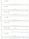 |
Fig. 1. Environment around the Paβ line in each spectrum. The data is shown in black along with the NEL fit (blue), BEL fit (green), continuum fit (red) and the sum of those fits (orange). |
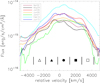 |
Fig. 2. Paβ BEL for our seven observation epochs. The color coding for the epochs is shown in the upper left corner of the plot. The subtraction of the NEL and continuum flux are described in Sect. 2. Wiggles can be seen for most epochs approximately at the center of the BEL. We cannot rule out that these are residuals from the NEL subtraction. Therefore it is not possible to tell whether these shape variations originate in the BLR. At the bottom of the figure the velocity bins used for Fig. 7 are shown and color coded from blue to red. The strongest shape variations can be seen in the red shifted part of the BEL especially around velocities of 2500 km s−1. |
3. BEL shape variation
3.1. Testing the temporal stability of the BEL profile
The evolution of BEL profiles across the seven epochs are presented in Figs. 2 (Paβ), 3 (O I 844 nm) and 4 (Brγ). Of these BELs, the Paβ line has the highest flux and S/N. The S/N of the O I 844 nm line is further reduced due to the higher continuum flux (so lower line-to-continuum-ratio) at these wavelengths compared to the Paβ line and especially at the Brγ line the continuum flux is much lower. Therefore, the further analysis is done for the Paβ line alone while it is done for the sum of the O I 844 nm and Brγ line to increase the S/N. The general findings are similar.
Apart from the overall flux changes a variation of the BEL shape can be seen in the red wings. During the first five epochs (from April 2002 to January 2007) a peak is apparent that flattens out with time and can no longer be seen in the February 2010 epoch. In the June 2015 epoch a similar peak appears again at the red wing. The apparent variations around the center of the BELs were already briefly addressed at the end of Sect. 2 and might be partly caused by residuals from the fit of the NELs. Our data does not sample strong shape variations in the blue wing. Similar emission peaks are found for the Hα and Hβ BELs of NGC 4151 by Shapovalova et al. (2010) at the same time as our IR spectra were taken at the red wings and also at earlier times in the red wings only.
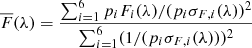
In order to measure the significance of these variations we used the rms profile of our spectra. For the classical rms approach the fitted NEL flux was normalized in order to have a constant NEL flux for all spectra and the April 2002 spectrum had to be excluded due to its lower spectral resolution. The resulting mean and rms profiles are shown in Fig. 5 along with a symmetrical BEL model which we develop in Sect. 4, based on the work of Stern et al. (2015). In Fig. 5 it becomes apparent that the mean profile of our Paβ emission line shows a significant shape discrepancy from the symmetrical profile in the red wing compared to the blue wing. Additionally the rms profile is slightly stronger in the red wing. If there were no shape variations it would be expected that the rms profile should be similar to the symmetrical profile. Nonetheless this approach of analyzing the rms spectral shape is not ideal to identify shape variations, since it mixes BEL flux variation with line profile shape variation.
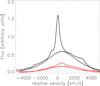 |
Fig. 5. Mean (black solid line) and rms (red solid line) profile for the Paβ line of all spectra despite the April 2002 spectrum (which had to be excluded here due to its lower spectral resolution). Along with this a model of a symmetrical BEL was plotted which we develop in Sect. 4 (red and black dotted lines) based on Stern et al. (2015). The gray dashed line shows the median flux error of individual pixels at the Paβ line. |
As we look for shape variation alone in these profiles we need to normalize the spectra in order to get rid of the overall flux changes of the BELs. For this it is necessary to subtract the constant part of the emission line, namely the NEL, first. We then introduced a fit parameter (which acts as a normalization factor) for each spectrum (pi) where the fit parameter for the May 2004 spectrum is fixed to 1.0. We then minimized the following rms profile: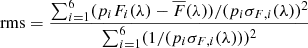 (1)
(1)
where Fi(λ) is the BEL flux and σF, i is the error of the BEL flux.  is the weighted mean flux of the seven spectra defined as
At first we determine the rms profile using the complete BELs. The resulting fit parameters pi are shown in Table 2 and the resulting rms (multiplied by a factor of three for better visibility) is shown in the left plot of Fig. 6 (dashed gray line) along with the spectra multiplied with their respective fit parameter (solid colored lines as in Fig. 2) and the weighted mean Flux (solid gray line). Looking at this rms profile we find two velocity ranges now where the variations are strong. For the first one around 0 km s−1 we can not easily tell to what extent these variations are real variations of the BELs or instead residuals from our NEL fit. Therefore we do not discuss them further here. The second peak of the rms profile is located in the region where the bumps discussed before can be seen from 2000 to 3000 km s−1.
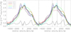 |
Fig. 6. Paβ BELs normalized with the fit parameters from the rms minimization Eq. (1) which are given in Table 2. The color coding of the BELs is given in the upper left corner. Additionally the mean spectrum (solid gray line) and the rms profile (dashed gray line) are shown. For better visibility the rms profile was multiplied by a factor of three. In the left plot the full BEL was used for the rms minimization. In order to make the minimization less sensitive to the shape variations of the BEL the indicated velocity ranges between −750 to 750 km s−1 and 2000 and 3000 km s−1 were excluded from the minimization in the right plot as the rms profile is largest in these regions indicating the strongest shape variations. |
In the next step, we excluded those velocity ranges where the rms profile peak and repeat the process determining the rms profile as shown above. We do this as we want to include only the parts of the BELs which do not change their shape in the fitting process to avoid a biased flux normalization. The results of this second iteration are shown in the right plot of Fig. 6 and the fit parameters  are given in Table 2. This does not strongly affect our fit parameters however pi is systematically smaller than
  with the exception of p0 and with
  having the largest increase. Especially on the blue wing the spectra are pushed together by this change. However at velocities between 0 and 2000 km s−1 the normalized flux of the May 2004 BEL (black line) is even further below the mean BEL while the normalized flux of the January 2007 BEL is even higher than the flux of the mean BEL. A similar behavior can be seen for the flux ratios compared to the May 2004 BEL. Excluding the varying parts of the BELs leads to a general increase in the flux ratios which is especially pronounced for the January 2007 BEL (compare rows 4 and 5 of Table 2).
We conclude that the BEL profile variation appears to be particularly pronounced between velocities of 2000 and 3000 km s−1.
3.2. Time evolution of the BEL profile
We divided our BELs in five equal velocity bins from −3250 to 4250 km s−1 (indicated by the symbols at the bottom of Figs. 2, 3, and 4). The bins are not centered around 0 km s−1 as the BELs are shifted by approximately 500 km s−1 with respect to the NELs. This velocity shift of the BELs with respect to the NEL center is also found by Shapovalova et al. (2010). We then integrated the flux in those bins as well as the overall flux from the BEL to get the ratio of those two values. This ratio is plotted in Fig. 7 over time for the Paβ BEL. Due to the lower S/N for the O I 844 nm and Brγ BELs we take the average of the ratios of the two lines for the same plot (Fig. 8). We decided not to take the sum of the fluxes to then get a combined average here as this would have lead to a higher weighting of the O I 844 nm line due to the higher flux of that BEL. The ratios are indicated by the different symbols which are also given at the bottom of the figures showing the BELs (Figs. 2–4).
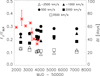 |
Fig. 7. Fluxes in different velocity bins (Fij) over the total flux from the Paβ BEL (Fi) over time for the seven spectra. The different symbols indicate the different velocity bins which are also given at the bottom of Fig. 2 and their central velocity is given at the top of the plot. The error bars are smaller than the symbols except for two of dust radii where the error bars are given. Indicated with the red stars are the radii of the last five epochs determined by Koshida et al. (2009). For those the reverberation delay in ld is plotted against time. At the same time the radius of the dust torus is reduced by a factor of approximately two, and the relative flux in the bin between 1250 and 2750 km s−1 (orange crosses) increases significantly. |
 |
Fig. 8. Same as Fig. 7 but for the sum of the ratios of the O I 844 nm and the Brγ BELs which are shown in Figs. 3 and 4. We use the sum of the two BELs to increase the S/N as the strength of those lines is much weaker than the Paβ line. A similar increase of the relative flux in the 1250–2750 km s−1 bin (filled squares) can be seen for the O I 844 nm and Brγ BEL. |
It can be seen in Fig. 7 that the relative flux in the central bin and the bin centered around 2000 km s−1 stays approximately constant between April 2002 and May 2004 and than gradually increases from the May 2004 BEL to the January 2007 BEL. The February 2010 BEL on the other hand shows an almost symmetrical BEL again (if 500 km s−1 is assumed as the center of the BEL). This supports the result from the rms profile of strong shape variations between May 2004 and January 2007. Additionally it shows that this change does not evolve randomly but the BEL flux in the red wing steadily increases.
Another feature in the BELs appears similar to an absorption of flux at 2000 km s−1 in the first period especially for the O I 844 nm and Brγ BEL. For the Paβ line it is not possible to tell whether the impression of a slightly lower flux is caused by the enhanced flux at 3000 km s−1. However as we definitely see this feature in two out of three BELs at the same velocities, this could be a real absorption-like feature. It is also possible that this is caused by a lower emission at these velocities. However the rms is significantly higher above 2000 km s−1 (compare Fig. 6) and we therefore concentrate on the variations between 2000 and 3000 km s−1. For the same reasons we neglect the slight shape variations in the blue wing. This shows that (slight) BEL shape variations are occurring throughout the BEL but are most significant between 2000 and 3000 km s−1. There are some shape variations around 0 km s−1 too, but these could be attributed to the NEL fit. Therefore, we cannot attribute these features cleanly to the BLR and we do not discuss them further in this paper.
4. Modeling BELs
Next we want to use the simple geometric parametrization of the BLR intensity distribution as described in Stern et al. (2015) to reproduce our BELs of NGC 4151. For the rest of the paper, we have used this approach to model the overall BEL profile, and extend it to realize the secondary peak observed. Of our seven spectra we chose the January 2006 spectrum as it is the highest S/N spectrum taken in the time period showing line profile variability. Additionally it shows a significant bump in the region were the rms profile is the highest (Fig. 6) and this spectrum was taken at a time when the radius of the dust torus determined by Koshida et al. (2009) was at a minimum. In total this BEL has the potential to provide the most information. The other BELs from this epoch show a similar overall width and a similar width of the bump (apart from the January 2007 BEL), although the bump intensity and location slightly changes. In order to do this we took Eq. (16) of Stern et al. (2015) describing the flux density of photons per unit velocity (v) that originate from the disk coordinate (r, φ):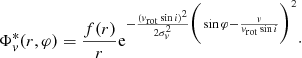 (3)
(3)
In this equation f(r) describes the radial distribution of the line emission while the exponential function describes the local line broadening due to the non-rotational velocity components (σv) in the BLR with i being the inclination between the accretion disk and the line of sight and vrot the rotational velocity (which is proportional to r−0.5 as the gravitational field is dominated by the central black hole).
In Fig. 3 of Stern et al. (2015) the influence of σv/(vrot sin i) on the shape of the BEL is shown. For values lower than one, the BEL is double peaked and for values above one the shape becomes single peaked without significant further changes for larger σv/(vrot sin i). Double peaked BELs are seen only if the FWHM reaches values above 10 000 km s−1 (e.g., Eracleous & Halpern 2003). Therefore we choose σv/(vrot sin i) = 1. The radial distribution of line emission is described by f(r)∝r1 for r < rBLR and f(r)∝r−1 for r > rBLR, where rBLR is the BLR radius measured with reverberation mapping. The changes of the BELs due to different radial distributions can be seen in Fig. 4 of Stern et al. (2015). We choose this distribution as it is the widest of the given distributions in Stern et al. (2015) and reproduces the overall shape of our BELs well. Thus we do not overestimate the rotational velocity of the BLR clouds. Applying a steeper radial profile, for example f(r)∝r±2, requires an increase of the rotational velocity by only 100 km s−1.
The inner and outer radius of the luminous BLR clouds are adopted from Baskin & Laor (2018) with values of rin = 0.18 rBLR and rout = 1.6 rBLR. The choice of rin and rout slightly influences the shape of the BEL as well. For example, a larger rout leads to additional relatively slow clouds inducing a narrower BEL hence increasing the necessary rotational velocity to reproduce the width of our BELs. A larger rin has a similar effect because the fastest clouds are removed. The inner and outer radii were determined for a constant AGN luminosity by Baskin & Laor (2018). However, the optical lightcurve of NGC 4151 (e.g., Shapovalova et al. 2008; Koshida et al. 2009) is not constant at all. Therefore BEL clouds might be present outside those radii depending on the earlier luminosities of NGC 4151 and the timescales on which BEL clouds are created and afterwards stop contributing to the BEL flux (for example by falling back to the accretion disk). As those timescales are not well understood, we use the radii from Baskin & Laor (2018).
This simple description of the BLR reproduces the overall shape of the Paβ lines very well. As the overall shape and width of the Paβ line does not change too much with time (compare Fig. 6) we only show the comparison to the January 2006 Paβ line in the upper left plot of Fig. 9. Shapovalova et al. (2010) also find that the FWHM of the BELs of NGC 4151 does not show strong changes (the FWHM only becomes smaller for a short time in 2000) despite the significantly reduced flux in a ten year span from 1996 to 2006.
 |
Fig. 9. Influence of some of the parameter space of Eq. (6) on the shape of the BEL in comparison to the observed January 2006 Paβ line (solid lines). In all plots the BEL was modeled with the parameters which reproduce the Paβ line best. These are vrot = 1500 km s−1, σv, 2 (vrot sin i)−1 = 0, vrot,2 = 2500 km s−1, σφ,2 ≈ 0.45 rad and φC, 2 = 0.5 π. The parameters varied are shown in the legends at the top of each plot. In the upper left plot the changes due to different rotational velocities are shown. The middle left plot illustrates how increasing the local line broadening leads to a wider bump. A visualization of the influence of a changing rotational velocity of the additional clouds is given in the right plot in the middle. In the lower left plot different widths of g(φ) are shown. We note that the dotted line is shifted down and the dashed dotted line is shifted up by 0.2 × 10⁻¹⁵ erg (s cm−2 Å) for better visibility. Finally in the lower left plot the center of the additional clouds (φC, 2) is varied. These plots are not to be understood as fits to the data. Rather we want to explore how different parameters change the modeled BEL. |
Next we want to reproduce the January 2006 spectrum with a separate peak around 2600 km s−1 in addition to the main Gaussian profile. We note that the center of the Paβ BEL is shifted by vshif = 500 km s−1 with respect to the center of the narrow line. The modeled flux was normalized to match the maximum observed flux in all plots of Fig. 9.
This process should not be understood as a fit to the data, which is difficult to interpret since the parameters are partly correlated. As we will show below, some of the elements of Eq. (3) have a similar effect on the BEL shape (e.g., the cloud distribution in r and vrot sin i). Therefore a fitting process could not distinguish between those parameters any way. Rather we want to explore how the Stern et al. (2015) description of the BLR has to be tweaked in order to reproduce such a narrow bump, to explore the spatial information encoded in the BEL velocities.
Equation 3 can well reproduce the BEL beside the bump and at velocities below −3000 km s−1 with vrot sin i = 1500 km s−1 (upper left plot of Fig. 9). To be able to describe features in the BELs like the peak present at the red part of the January 2006 Paβ line (compare also Fig. 2) we need to vary the cloud distribution in azimuthal direction as well, adding a function g(φ) to Eq. (3):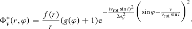 (4)
(4)
We chose a Gaussian distribution centered around φC, 2 = 0.5 π with its width denoted by σφ, 2 from hereon: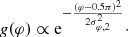 (5)
(5)
The distribution in φ is shown in Fig. 10 for the different widths used in the lower left plot of Fig. 9. Apart from the lower left plot we always choose the width of the additional bump to be  in Fig. 9.
 |
Fig. 10. Distribution of additional clouds in the BLR introduced by g(φ) in Eq. (4) and (6) in azimuthal direction. These additional clouds are needed to reproduce the bump in the January 2006 spectrum in Fig. 2 (red line). They are modeled as a Gaussian distribution with a width of σφ, 2 = 0.20, 0.45 and 0.70 rad and centered around φC, 2 = 0.5 π. |
However the local line broadening acts as a convolution on g(φ). Therefore however small we choose the region in φ, where gas clouds in addition to the symmetric distribution are located, the contribution to the overall flux extends over a larger range of velocities compared to the January 2006 peak. This effect is shown in the middle left plot of Fig. 9. For values of σv, 2/(vrot, 2sini)= 0.25 and 1 (dotted line and dashed line) the additional flux extends over a large velocity range. Only if σv, 2/(vrot, 2sini) goes to zero we can reproduce the bump properly. Hence we have to change the local line broadening term for the clouds described in g(φ): (6)
(6)
A summary of the parameter space of this equation is given in Table 3.
The local line broadening does not have to vanish altogether. In fact the width of the peak depends as well on the distribution of clouds in radial and azimuthal direction. But with the delta function we get an upper limit on the volume of the additional clouds in φ. With the same argument, we changed the distribution in r to a steeper distribution with f2(r)∝r2 for r < rBLR and f2(r)∝r−2 for r > rBLR. The radial distribution of line emission is shown in Fig. 11 for f, f2 and the sum of the two components at φC, 2. The flux originating from this additional bump is responsible for about 5% of the total BEL flux.
 |
Fig. 11. Radial distribution of line emission as used in Eq. (6) for f (red line), f2 (blue line) and the sum of the two components at φ = 0.5 π (where we put the additional clouds in azimuthal direction). rrm is the center of the overall BLR and the additional clouds are shifted inwards according to the ratio of vrot and vrot, 2 squared. Together with the distribution in azimuthal direction (compare Fig. 10) the additional clouds are responsible for approximately 5% of the total BEL flux. |
Even if we chose these clouds to be located at φC, 2 = 0.5 π where vrot sin i is directed exactly away from us (the unprojected velocity is proportional to sinφ) we would not be able to reach velocities above 1500 km s−1. However the peak can be best reproduced with a velocity of 2500 km s−1 as shown in middle right plot of Fig. 9. Therefore the additional clouds responsible for the bump emission need to be located closer to the black hole than rBLR as a rotational velocity of at least vrot sin i = 2500 km s−1 is needed to create a peak at this velocity. Therefore, a second velocity must be introduced in Eq. (6) (vrot, 2) which is the velocity of the additional clouds added with g(φ).
In the lower left plot of Fig. 9, we show how changes of the width of g(φ) changes the appearance of our bump. Apart from the peak becoming slightly wider with increasing width it does not change too strongly. The reason for this is the non-existing local line broadening. As long as the local line broadening is turned off, a constant cloud distribution in azimuthal direction leads to a double peaked BEL. This means the distinct peak around vrot, 2sini will not show major changes to its width however big we choose  . Yet σφ,2 ≈ 0.45 rad gives us the best resulting peak and if the additional clouds would be extended throughout the accretion disk there should be a second peak at the blue shifted wing of the BEL.
The results for a varying φC, 2 is shown in the lower right plot. Moving the center towards 0 has two effects: The resulting peak widens and the center of the peak moves towards lower velocities. But unless σφ, 2 is not very small the velocity change of the peak is smaller than sin φC, 2 would suggest due to the convolution with the local line broadening term. However if we choose σφ, 2 too small it can be hard to explain how to produce 5% of the BEL flux in such a small space on timescales of at most two years. For φC, 2 < 0 the same peaks appear on the blue wing of the BEL.
There are three effects which could lead to the subsequent flattening of the peak in June 2006 and January 2007: The clouds rotating away from φC, 2 = 0.5 π (which would take longer than one year at these rotational velocities), turning on the local line broadening again (the clouds of g(φ) no longer move with a common velocity) and additional similar events at lower projected velocities or a combination of these two effects. A further extend of the clouds in azimuthal direction can not explain this broadening alone as the small local line broadening always leads to a peak around vrot, 2sini (compare the lower right plot of Fig. 9). The enhanced flux in January 2007 extends to around the center of the BEL. As we can see in the upper right plot of Fig. 9 this can be realized with  and local line broadening term of σv, 2 (vrot sin i)−1 = 0.25.
5. Discussion
In this chapter, we explore if the so far purely phenomenological description of BEL profile variability in NGC 4151 matches our understanding of physical processes occurring in that very central region around the SMBH.
5.1. Dust production
In Fig. 7, we show the dust radii of NGC 4151 (red stars) determined by Koshida et al. (2009) along with the increasing relative flux in the red wing of the BELs. This parallel change of BEL shape and dust radius in NGC 4151 raises the question whether this is coincidental or is caused by a connection between the BLR and the dust torus and what this can tell us about dust occurrence and creation in AGN. An important property for the dust creation is the temperature of the dust torus. Only below a certain temperature dust can be created. This limiting temperature is usually assumed to be around 1000 K (e.g., Czerny & Hryniewicz 2011) as this temperature was found for dust production in outflows of evolved stars where similar conditions are present as in BLR clouds (Groenewegen et al. 2009). Unfortunately Koshida et al. (2009) could not measure the temperature directly as they only had single band infrared fluxes in the K band. However applying equation 1 from Kishimoto et al. (2007) the dust temperature can be connected to the dust radius (Rsub, theo), the UV luminosity (LUV), the sublimation temperature (Tsub) and the grain size of the dust (a): (7)
(7)
Assuming a constant dust grain size and sublimation temperature for NGC 4151 we can calculate mean dust temperatures at different radii if we assume certain temperatures in one of the periods from Koshida et al. (2009). Our chosen period is the third one, as its luminosity is the highest while the dust radius is comparable to the first period where the luminosity is much lower. Therefore we can assume that the dust temperature should not be very low in the third period. We want to see which temperature a dust cloud at the smallest dust radius found by Koshida et al. (2009) (33 ld) would have during all periods: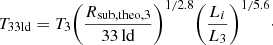 (8)
(8)
In this equation T3 is the assumed mean temperature in the third period, Rsub, theo, 3 is the sublimation radius during the third period and Li is the mean luminosity in different epochs. With Eq. (8) we get the temperature at different times at a distance of 33 ld to the black hole.
The result of this line of thought is shown in Fig. 12 for T3 between 1000 and 1500 K. During the second period Landt et al. (2015) measured a dust temperature of 1316 K. During the third epoch the luminosity is higher while the dust radius stays almost the same. Therefore dust temperatures should be higher than 1300 K. Additionally the temperatures measured by Schnülle et al. (2015) and Landt et al. (2015) for NGC 4151 never drop below 1200 K. Baskin & Laor (2018) show that depending on especially gas density, grain size, and dust type Tsub can reach temperatures as high as 2000 K. Therefore the temperature T3 can be assumed to be at least higher than 1300 K.
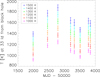 |
Fig. 12. Different dust temperatures for NGC 4151 at a distance of 33 ld from the black hole assuming mean temperatures between 1000 and 1500 K during the third epoch of the NGC 4151 dust reverberation campaign from Koshida et al. (2009). The temperatures were calculated using Eq. (8) with the assumption of a constant dust grain size. The color coding for the assumed mean temperatures during the third reverberation period is shown in the upper left corner of the plot. This shows that it is very hard to reach temperatures below 1000 K at a distance of 33 ld from the black hole, which are needed for dust production above the accretion disk. |
This means it is very hard to create dust above the accretion disk at the radii where dust reverberation finds it. In Fig. 12 it can be seen that a temperature below 1000 K can only be reached if T3 is as low as ∼1000 K and only in the sixth period (apart from the first period). Otherwise the temperatures are well above this threshold for dust production at a distance of 33 ld from the black hole. If T3 is indeed higher than 1300 K the mean temperatures at this distance to the black hole can not be much smaller than 1200 K. Therefore it is only possible to form the dust above the accretion disk if dust formation can happen on very short timescales when the temperature is (significantly) below the mean temperature. If the dust were to be produced by stars outside the AGN as proposed by Schartmann et al. (2010) in NGC 1068 the decrease of the dust radius of ∼30 ld in ∼600 days would suggest a velocity of the dusty gas clouds towards the black hole of approximately 5% of the speed of light. This seems to be too high for an inflow as only ultra fast outflows from AGN have been observed in this velocity range. Velocities in a range up to 30% the speed of light peaking around 0.1% the speed of light were reported for these outflows (e.g., Chartas et al. 2003; Tombesi et al. 2010).
A solution to this problem (finding dust where it is too hot to form it) is provided by the model of the outer BLR formation from Czerny & Hryniewicz (2011). The dust is formed inside the accretion disk where the radiation from the inner accretion disk is blocked by the accretion disk and therefore temperatures can be lower than above the accretion disk where the clouds are directly exposed to the accretion disk. The dusty clouds are than pushed above the accretion disk where the clouds are directly exposed to the radiation from the inner accretion disk and subsequently destroyed by the radiation if the clouds are heated above the sublimation temperature. If the dust is indeed destroyed the gas clouds can become visible as part of the BEL.
This relates to the changes of the dust radius and the shape of the BEL as follows. Dust clouds are produced within a range of radii in the accretion disk smaller than the previously smallest dust radius (sublimation radius) above the accretion disk due to the additional radiation shielding inside the disk. Of these emerged dusty clouds the innermost clouds will loose their dust due to sublimation quickly and appear as addition to the BLR, while the dusty clouds will survive longer at small radii. If the amount of dust clouds is high enough, or the accretion disk luminosity drops at the same time these dusty clouds will lead to a reduced time lag of the dust reverberation radius as seen by Koshida et al. (2009). Thus the same cloud formation process in a radiation driven wind can add both to the BLR gas clouds, and the dusty clouds contributing to the torus.
5.2. Kinematic features and possible origin of additional clouds
The results from our BEL modeling (compare with Section 4) support the view discussed above. The radius at which the shape of the BEL changes has to be at least two times smaller than rBLR of the overall BEL because of the velocities of the overall BEL and the additional peak. This is comparable to the changes in dust radius found by Koshida et al. (2009). The enhanced flux can only be seen around 2100 km s−1 in the BELs while the overall shape of the BELs does not change much with rotational velocities of around vrot sin i = 1500 km s−1. An explanation for this is that the BEL changes only in a confined area in azimuthal direction of the accretion disk and the overall distribution changes take much longer. It could be possible to explain the enhanced BEL gas density by an inflow of gas clouds, but in this case the changes in the shape on timescales of half a year from January 2006 to June 2006 and January 2007 are hard to explain.
The overall distribution of BEL clouds would not be symmetrical under these assumptions. In Fig. 9 we showed that a broader distribution of additional clouds still leads to a distinct peak as long as the local line broadening term is negligible. Therefore it is hard to pinpoint how broad the distribution of additional clouds is as the width in flux of the additional peak is not very sensitive to this distribution. Nonetheless a width of σφ,2 ≈ 0.45 rad can best reproduce the peak found in the January 2006 BEL and if we increase the local line broadening term again we can reproduce a wider additional flux without changing σφ, 2 as seen in the January 2007 Paβ BEL. In 2010 the bump vanished completely which can be caused by a combination of two effects: a further increase of the local line broadening term and a dispersion of clouds in azimuthal direction due to interactions with other BLR clouds. While there is no chance to get this azimuthal information of the distribution of dust clouds Schnülle et al. (2015) found indications of a radial extend of the inner edge of the dust torus as well in NGC 4151 (although not at the same time). It could be interesting to see whether simulations can reproduce the changes in dust radius even if the “new” dust has only a similarly small extend in azimuthal direction.
We can also infer an absolute value of rBLR for the two velocities we got from our modeling using the black hole mass determined by Grier et al. (2013) of 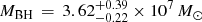 . This leads to
 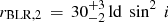 for vrot,2 sin i = 2500 km s−1 and
  for vrot sin i = 1500 km s−1. In the literature the inclination is given as 45° with an error around 10° (e.g., Das et al. 2005; Müller-Sánchez et al. 2011) and thus sin2i leads to a factor of 0.5 and hence radii of the BLR around 15 and 40 ld. These radii lie well within the range in which Shapovalova et al. (2008) found emitting gas (1–50 ld) between 1996 and 2006.
According to Baskin & Laor (2018) the outer radius of the BLR is located at 1.6 rBLR. This leads to an outer radius of the BLR or inner dust radii of 66 ± 15 ld and 24 ± 5 ld. Both of these values are slightly lower than the largest and smallest dust radius found by Koshida et al. (2009) (71 and 33 ld). However, Schnülle et al. (2013) showed that the determined dust radius depends on the infrared wavelength used for the dust reverberation mapping. As Koshida et al. (2009) used the K band they will not have picked up this innermost dust radius. Therefore our determined rBLR is not in contradiction with their dust radius. The flux present in the peak is responsible for about 5% of the total BEL flux and the area in which this flux is produced (with a width of σφ,2 ≈ 0.45 rad and at a smaller radius) is also in the range of 5% the area in which the overall BEL was produced. This shows that the area should be large enough to produce the additional flux.
With this radius we can also determine a temperature inside the accretion disk following the line of argument of Czerny & Hryniewicz (2011) using the monochromatic luminosity at 5100 Å. We can take this luminosity from Shapovalova et al. (2008) and get a disk temperature of around 450 K at rin. However looking at the optical lightcurve in both Shapovalova et al. (2008) and Koshida et al. (2009) of NGC 4151, the optical flux was significantly higher in December 2005 (with no data until June 2005). As the clouds are produced before becoming visible as part of the BEL we can get to temperatures of approximately 600 K easily considering an increased monochromatic luminosity (or potentially even higher if the optical flux would have been even higher between June and December 2005). This temperature is consistent with the dispersion of temperatures found by Czerny & Hryniewicz (2011), who published a similar temperature of 550 K for NGC 4151. To summarize, while at the centro-nuclear radii, where we locate the clouds responsible for the BLR shape variation, the temperatures above the accretion disk appear too high for in situ dust formation, they drop to values allowing to form dust inside the accretion disk of NGC 4151 at the same radii.
6. Summary and conclusions
We connected BEL shape variability to the decrease of the dust radius in NGC 4151 between May 2004 and January 2006 in this paper. The results we obtain are:
-
The simultaneous decrease of the dust radius and BEL shape variability point to a connection between the BLR and the dust torus. Additionally the velocity, at which the shape variability occurs, indicates a similar decrease of dust radius and BLR radius.
-
The dust needed for the reduced dust radius is presumably produced in the accretion disk as the temperatures above the accretion disk hardly reach temperatures low enough for dust production. Inflows are also unlikely as a reason for the change of dust radius due to the short timescales of the changes of dust radius. This leaves us with dust production in the accretion disk described in dust inflated accretion disk models. The indications for a similar decrease in radius of both the clouds of the dust torus and BLR provide evidence that the dust and BLR clouds share a similar origin.
-
The correlated changes in the BEL discussed occur in only a small range of velocities (visible as transient bump). This indicates missing broadening via velocity dispersion of the fresh clouds which can be naturally explained by the here favored formation scenario in an accretion disk wind. We cannot significantly constrain the azimuthal extension of the cloud formation zone but can rule out a completely symmetrical distribution all around the nucleus. If the dust torus and BLR are indeed similar in their production mechanism it is possible that the dust torus shows a similar distribution of clouds.
-
The location of peaks in BELs can give us information of the radial position of the BLR. In particular if the peak is well defined and sharp the probability is high that the additional clouds are located close to φ = ± 0.5 π. For azimuthal angles with lower projected velocities the peak would be broadened and a much smaller extend in azimuthal direction of the additional clouds would be needed. This explains why similar cloud formation events are less observable if occurring at different azimuthal angles.
As this is only one occasion where we were able to observe the described scenario, we cannot (and do not want to) rule out other dust production outside of the accretion disk in other objects, at other times or at higher radii than those investigated here. For the same reason we cannot speculate what might cause the changes in dust production or if these are just statistical variations. In contrast, our analysis of combined datasets shows evidence supporting dust production in the accretion disk and a similar production mechanism of the dust torus and BLR. For future campaigns, it is important to observe the BLR and dust torus at the same time and with sufficient temporal sampling (bi-weekly for Seyfert-type AGN) in order to robustly detect similar events. Modern extremely-wide-band spectrographs, delivering optical-near-infrared in one shot (like the VLT X-shooter) are most adequate to achieve this. Such data will help to improve our understanding of dust creation in AGN and how the radius of the dust torus and the BLR changes.
References
- Antonucci, R. 1993, ARA&A, 31, 473 [Google Scholar]
- Bannikova, E. Y., Vakulik, V. G., & Sergeev, A. V. 2012, MNRAS, 424, 820 [NASA ADS] [CrossRef] [Google Scholar]
- Barvainis, R. 1987, ApJ, 320, 537 [NASA ADS] [CrossRef] [Google Scholar]
- Baskin, A., & Laor, A. 2018, MNRAS, 474, 1970 [NASA ADS] [CrossRef] [Google Scholar]
- Bentz, M. C., Peterson, B. M., Pogge, R. W., Vestergaard, M., & Onken, C. A. 2006, ApJ, 644, 133 [NASA ADS] [CrossRef] [Google Scholar]
- Chartas, G., Brandt, W. N., & Gallagher, S. C. 2003, ApJ, 595, 85 [NASA ADS] [CrossRef] [Google Scholar]
- Cushing, M. C., Vacca, W. D., & Rayner, J. T. 2004, PASP, 116, 362 [NASA ADS] [CrossRef] [Google Scholar]
- Czerny, B., & Hryniewicz, K. 2011, A&A, 525, L8 [NASA ADS] [CrossRef] [EDP Sciences] [Google Scholar]
- Czerny, B., Li, Y.-R., Hryniewicz, K., et al. 2017, ApJ, 846, 154 [NASA ADS] [CrossRef] [Google Scholar]
- Das, V., Crenshaw, D. M., Hutchings, J. B., et al. 2005, AJ, 130, 945 [NASA ADS] [CrossRef] [Google Scholar]
- Eracleous, M., & Halpern, J. P. 2003, ApJ, 599, 886 [NASA ADS] [CrossRef] [Google Scholar]
- Grier, C. J., Martini, P., Watson, L. C., et al. 2013, ApJ, 773, 90 [CrossRef] [Google Scholar]
- Groenewegen, M. A. T., Sloan, G. C., Soszyński, I., & Petersen, E. A. 2009, A&A, 506, 1277 [NASA ADS] [CrossRef] [EDP Sciences] [Google Scholar]
- Hönig, S. F., & Kishimoto, M. 2010, A&A, 523, A27 [NASA ADS] [CrossRef] [EDP Sciences] [Google Scholar]
- Hönig, S. F., Watson, D., Kishimoto, M., et al. 2017, MNRAS, 464, 1693 [NASA ADS] [CrossRef] [Google Scholar]
- Ilić, D., Popović, L. Č., Shapovalova, A. I., et al. 2015, JA&A, 36, 433 [NASA ADS] [Google Scholar]
- Kaspi, S., Smith, P. S., Netzer, H., et al. 2000, ApJ, 533, 631 [NASA ADS] [CrossRef] [Google Scholar]
- Kishimoto, M., Hönig, S. F., Beckert, T., & Weigelt, G. 2007, A&A, 476, 713 [NASA ADS] [CrossRef] [EDP Sciences] [Google Scholar]
- Koshida, S., Yoshii, Y., Kobayashi, Y., et al. 2009, ApJ, 700, L109 [NASA ADS] [CrossRef] [Google Scholar]
- Landt, H., Bentz, M. C., Ward, M. J., et al. 2008, ApJS, 174, 282 [NASA ADS] [CrossRef] [Google Scholar]
- Landt, H., Bentz, M. C., Peterson, B. M., et al. 2011a, MNRAS, 413, L106 [NASA ADS] [CrossRef] [Google Scholar]
- Landt, H., Elvis, M., Ward, M. J., et al. 2011b, MNRAS, 414, 218 [NASA ADS] [CrossRef] [Google Scholar]
- Landt, H., Ward, M. J., Steenbrugge, K. C., & Ferland, G. J. 2015, MNRAS, 449, 3795 [NASA ADS] [CrossRef] [Google Scholar]
- Lira, P., Botti, I., Kaspi, S., & Netzer, H. 2018, ArXiv e-prints [arXiv:1801.03866] [Google Scholar]
- Müller-Sánchez, F., Prieto, M. A., Hicks, E. K. S., et al. 2011, ApJ, 739, 69 [NASA ADS] [CrossRef] [Google Scholar]
- Nenkova, M., Ivezić, Ž., & Elitzur, M. 2002, ApJ, 570, L9 [NASA ADS] [CrossRef] [Google Scholar]
- Nenkova, M., Sirocky, M. M., Ivezić, Ž., & Elitzur, M. 2008, ApJ, 685, 147 [NASA ADS] [CrossRef] [Google Scholar]
- Rayner, J. T., Toomey, D. W., Onaka, P. M., et al. 2003, PASP, 115, 362 [NASA ADS] [CrossRef] [Google Scholar]
- Riffel, R., Rodríguez-Ardila, A., & Pastoriza, M. G. 2006, A&A, 457, 61 [NASA ADS] [CrossRef] [EDP Sciences] [Google Scholar]
- Schartmann, M., Meisenheimer, K., Camenzind, M., Wolf, S., & Henning, T. 2005, A&A, 437, 861 [NASA ADS] [CrossRef] [EDP Sciences] [Google Scholar]
- Schartmann, M., Burkert, A., Krause, M., et al. 2010, MNRAS, 403, 1801 [NASA ADS] [CrossRef] [Google Scholar]
- Schnülle, K., Pott, J.-U., Rix, H.-W., et al. 2013, A&A, 557, L13 [NASA ADS] [CrossRef] [EDP Sciences] [Google Scholar]
- Schnülle, K., Pott, J.-U., Rix, H.-W., et al. 2015, A&A, 578, A57 [NASA ADS] [CrossRef] [EDP Sciences] [Google Scholar]
- Shapovalova, A. I., Popović, L. Č., Collin, S., et al. 2008, A&A, 486, 99 [NASA ADS] [CrossRef] [EDP Sciences] [Google Scholar]
- Shapovalova, A. I., Popović, L. Č., Burenkov, A. N., et al. 2010, A&A, 509, A106 [NASA ADS] [CrossRef] [EDP Sciences] [Google Scholar]
- Stern, J., Hennawi, J. F., & Pott, J.-U. 2015, ApJ, 804, 57 [NASA ADS] [CrossRef] [Google Scholar]
- Suganuma, M., Yoshii, Y., Kobayashi, Y., et al. 2006, ApJ, 639, 46 [NASA ADS] [CrossRef] [Google Scholar]
- Sulentic, J. W., Marziani, P., & Dultzin-Hacyan, D. 2000, ARA&A, 38, 521 [NASA ADS] [CrossRef] [Google Scholar]
- Tombesi, F., Cappi, M., Reeves, J. N., et al. 2010, A&A, 521, A57 [NASA ADS] [CrossRef] [EDP Sciences] [Google Scholar]
- Urry, C. M., & Padovani, P. 1995, PASP, 107, 803 [NASA ADS] [CrossRef] [Google Scholar]
- Vacca, W. D., Cushing, M. C., & Rayner, J. T. 2003, PASP, 115, 389 [NASA ADS] [CrossRef] [Google Scholar]
- Watson, D., Denney, K. D., Vestergaard, M., & Davis, T. M. 2011, ApJ, 740, L49 [NASA ADS] [CrossRef] [Google Scholar]
- Wildy, C., Landt, H., Goad, M. R., Ward, M., & Collinson, J. S. 2016, MNRAS, 461, 2085 [NASA ADS] [CrossRef] [Google Scholar]
All Tables
All Figures
|
Fig. 1. Environment around the Paβ line in each spectrum. The data is shown in black along with the NEL fit (blue), BEL fit (green), continuum fit (red) and the sum of those fits (orange). |
| In the text | |
|
Fig. 2. Paβ BEL for our seven observation epochs. The color coding for the epochs is shown in the upper left corner of the plot. The subtraction of the NEL and continuum flux are described in Sect. 2. Wiggles can be seen for most epochs approximately at the center of the BEL. We cannot rule out that these are residuals from the NEL subtraction. Therefore it is not possible to tell whether these shape variations originate in the BLR. At the bottom of the figure the velocity bins used for Fig. 7 are shown and color coded from blue to red. The strongest shape variations can be seen in the red shifted part of the BEL especially around velocities of 2500 km s−1. |
| In the text | |
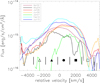 |
Fig. 3. Same as Fig. 2 for the O I 844 nm BEL. |
| In the text | |
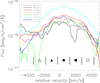 |
Fig. 4. Same as Fig. 2 for the Brγ BEL. |
| In the text | |
|
Fig. 5. Mean (black solid line) and rms (red solid line) profile for the Paβ line of all spectra despite the April 2002 spectrum (which had to be excluded here due to its lower spectral resolution). Along with this a model of a symmetrical BEL was plotted which we develop in Sect. 4 (red and black dotted lines) based on Stern et al. (2015). The gray dashed line shows the median flux error of individual pixels at the Paβ line. |
| In the text | |
|
Fig. 6. Paβ BELs normalized with the fit parameters from the rms minimization Eq. (1) which are given in Table 2. The color coding of the BELs is given in the upper left corner. Additionally the mean spectrum (solid gray line) and the rms profile (dashed gray line) are shown. For better visibility the rms profile was multiplied by a factor of three. In the left plot the full BEL was used for the rms minimization. In order to make the minimization less sensitive to the shape variations of the BEL the indicated velocity ranges between −750 to 750 km s−1 and 2000 and 3000 km s−1 were excluded from the minimization in the right plot as the rms profile is largest in these regions indicating the strongest shape variations. |
| In the text | |
|
Fig. 7. Fluxes in different velocity bins (Fij) over the total flux from the Paβ BEL (Fi) over time for the seven spectra. The different symbols indicate the different velocity bins which are also given at the bottom of Fig. 2 and their central velocity is given at the top of the plot. The error bars are smaller than the symbols except for two of dust radii where the error bars are given. Indicated with the red stars are the radii of the last five epochs determined by Koshida et al. (2009). For those the reverberation delay in ld is plotted against time. At the same time the radius of the dust torus is reduced by a factor of approximately two, and the relative flux in the bin between 1250 and 2750 km s−1 (orange crosses) increases significantly. |
| In the text | |
|
Fig. 8. Same as Fig. 7 but for the sum of the ratios of the O I 844 nm and the Brγ BELs which are shown in Figs. 3 and 4. We use the sum of the two BELs to increase the S/N as the strength of those lines is much weaker than the Paβ line. A similar increase of the relative flux in the 1250–2750 km s−1 bin (filled squares) can be seen for the O I 844 nm and Brγ BEL. |
| In the text | |
|
Fig. 9. Influence of some of the parameter space of Eq. (6) on the shape of the BEL in comparison to the observed January 2006 Paβ line (solid lines). In all plots the BEL was modeled with the parameters which reproduce the Paβ line best. These are vrot = 1500 km s−1, σv, 2 (vrot sin i)−1 = 0, vrot,2 = 2500 km s−1, σφ,2 ≈ 0.45 rad and φC, 2 = 0.5 π. The parameters varied are shown in the legends at the top of each plot. In the upper left plot the changes due to different rotational velocities are shown. The middle left plot illustrates how increasing the local line broadening leads to a wider bump. A visualization of the influence of a changing rotational velocity of the additional clouds is given in the right plot in the middle. In the lower left plot different widths of g(φ) are shown. We note that the dotted line is shifted down and the dashed dotted line is shifted up by 0.2 × 10⁻¹⁵ erg (s cm−2 Å) for better visibility. Finally in the lower left plot the center of the additional clouds (φC, 2) is varied. These plots are not to be understood as fits to the data. Rather we want to explore how different parameters change the modeled BEL. |
| In the text | |
|
Fig. 10. Distribution of additional clouds in the BLR introduced by g(φ) in Eq. (4) and (6) in azimuthal direction. These additional clouds are needed to reproduce the bump in the January 2006 spectrum in Fig. 2 (red line). They are modeled as a Gaussian distribution with a width of σφ, 2 = 0.20, 0.45 and 0.70 rad and centered around φC, 2 = 0.5 π. |
| In the text | |
|
Fig. 11. Radial distribution of line emission as used in Eq. (6) for f (red line), f2 (blue line) and the sum of the two components at φ = 0.5 π (where we put the additional clouds in azimuthal direction). rrm is the center of the overall BLR and the additional clouds are shifted inwards according to the ratio of vrot and vrot, 2 squared. Together with the distribution in azimuthal direction (compare Fig. 10) the additional clouds are responsible for approximately 5% of the total BEL flux. |
| In the text | |
|
Fig. 12. Different dust temperatures for NGC 4151 at a distance of 33 ld from the black hole assuming mean temperatures between 1000 and 1500 K during the third epoch of the NGC 4151 dust reverberation campaign from Koshida et al. (2009). The temperatures were calculated using Eq. (8) with the assumption of a constant dust grain size. The color coding for the assumed mean temperatures during the third reverberation period is shown in the upper left corner of the plot. This shows that it is very hard to reach temperatures below 1000 K at a distance of 33 ld from the black hole, which are needed for dust production above the accretion disk. |
| In the text | |
Current usage metrics show cumulative count of Article Views (full-text article views including HTML views, PDF and ePub downloads, according to the available data) and Abstracts Views on Vision4Press platform.
Data correspond to usage on the plateform after 2015. The current usage metrics is available 48-96 hours after online publication and is updated daily on week days.
Initial download of the metrics may take a while.