| Issue |
A&A
Volume 621, January 2019
|
|
|---|---|---|
| Article Number | A11 | |
| Number of page(s) | 31 | |
| Section | Extragalactic astronomy | |
| DOI | https://doi.org/10.1051/0004-6361/201833508 | |
| Published online | 19 December 2018 | |
Possible evidence of a supermassive black hole binary with two radio jets in blazar 3C279
1
Max-Planck Institüt für Radioastronomie, Auf dem Hügel 69, 53121
Bonn, Germany
2
National Astronomical Observatories, Chinese Academy of Sciences, 100012
Beijing, PR China
e-mail: This email address is being protected from spambots. You need JavaScript enabled to view it.
Received:
28
May
2018
Accepted:
19
July
2018
Abstract
Context. Studies of periodic and quasi-periodic phenomena in optical and radio bands are important for understanding the physical processes in quasars. Investigation of periodic/quasi-periodic behavior of the relativistic jets in blazars is particularly significant because it can provide unique information about the formation, collimation, and acceleration of the jets and the properties of the central engines (black hole/accretion disk systems) in blazars.
Aims. We investigate the parsec-scale kinematics of the 31 superluminal components observed in blazar 3C279 and attempt to search for evidence of its jet precession and double-jet structure.
Methods. The previously suggested precessing jet nozzle model is applied to model-fit the kinematics of its superluminal components observed during the 1981–2015 period. It is shown that the parsec-scale kinematics of the entire source can be interpreted in terms of a double-jet scenario.
Results. The superluminal components observed in 3C279 can be divided into two groups that are ejected from two relativistic jets. The two jets have different orientations in space and jet-cone shapes, but both jets precess with the same precession period of 25 yr (16.3 yr in the source frame). The kinematic features of all the superluminal knots (trajectory, core separation, and apparent velocity) can be consistently explained. Their innermost trajectories follow the respective precessing common parabolic patterns with trajectory curvatures that occurred in the outer jet regions at different core separations. The bulk Lorentz factor, Doppler factor, and viewing angle of their motion are derived. The unusual jet-direction change of ∼100° observed in 2010–2011 can be naturally explained.
Conclusions. We propose a double-jet structure scenario for 3C279 and suggest that there may be a supermassive black hole binary in the center of 3C279 ejecting two precessing relativistic jets, resulting in its very complex structure and kinematics on parsec scales, and with extremely variable emission across the electromagnetic spectrum. Because the two jets have the same precession period, the precession of the double jet may have originated from the modulation of their jet orientation by the change in their orbital velocity direction relative to the observer. In this case the mass ratio m/M of the binary is approximately equal to the ratio of the jet cone widths, being on the order of ∼0.5.
Key words: galaxies: active / galaxies: nuclei / quasars: individual: 3C279
© ESO 2018
1. Introduction
Research on blazars is an important extragalactic astrophysical field in which extensive observations of their radiation from radio to γ rays are carried out and the mechanisms of radiation are studied (e.g., Abdo et al. 2010; Begelman et al. 1980; Blandford & Znajek 1977; Blandford & Payne 1982; Jorstad & Marscher 2016; Jorstad et al. 2017; Chatterjee et al. 2012, 2008; Lewis et al. 2018; Li et al. 1992; Marscher et al. 2017, 2012, 2010; Marscher & Jorstad 2011; Meier et al. 2001; Meier & Nakamura 2006; Petropoulou et al. 2016, 2017; Raiteri et al. 2010; Schinzel et al. 2010; Vercellone et al. 2010; Vlahakis & Koenigl 2004; Qian 2013, 2015, 2016; Qian et al. 2009, 2010, 2014, 2017, 2018). These studies have led to many important results for blazar physics, especially for the various physical processes occurring in the relativistic jets and the central black hole/accretion disk systems.
Blazar 3C279 (z = 0.538) is a flat-spectrum radio quasar (FSRQ) and is one of the most prominent blazars that has been intensively observed and well studied. It has also been categorized as an optically violent variable (OVV) revealing large and rapid polarized outbursts in optical bands on various timescales (days to years). Multifrequency radio light curves (4.8 GHz–36.8 GHz) have been used to study the core shift effect and to estimate the equipartition field strength and the spin of its black hole (Agarwal et al. 2017). Based on the measurements of its spectral lines (luminosity and line width) the mass of its central black hole has been estimated to be 108.9 ± 0.5 M⊙ (Nilsson et al. 2009; Gu et al. 2001; Woo & Urry 2002).
3C279 radiates across the entire electromagnetic spectrum from radio through optical and X-ray to γ rays. Very strong variability is observed in all these wavebands on various timescales (hours/days to years). Based on intensive multiwavelength observations and very long baseline interferometry (VLBI) monitorings, studies of the correlation between outbursts at radio, optical/IR, X-ray, and γ-ray wavelengths have provided important information on its variability properties, especially the radiation mechanisms for its X-ray and γ-ray emission and their locations in the jet (e.g., Collmar et al. 2010; Chatterjee et al. 2012; Agudo et al. 2011; Aleksić et al. 2014; Cohen et al. 2014; Isler et al. 2017). Multiwavelength campaigns and studies (e.g., Collmar et al. 2010; Rani et al. 2017; Hayashida et al. 2012, 2015; Kang et al. 2015; Larionov et al. 2008) have been performed to explore the spectral energy distribution (SED) of its broadband emission. Its SED consists of two bumps, one at IR-optical bands and the other at the Gev γ-ray band. This radiation structure can usually be interpreted in the one-zone leptonic scenario (e.g., Jorstad et al. 2007; Marscher 2008, 2009; Marscher & Jorstad 2011; Marscher et al. 2012; Abdo et al. 2010; Chatterjee et al. 2012): the lower frequency bump originates from synchrotron emission of relativistic electrons in magnetic fields and the high-frequency bump originates from inverse-Compton scattering of the synchrotron photons (synchrotron self-Compton (SSC) process, Maraschi et al. 1992; Arbeiter et al. 2005) or inverse-Compton scattering of external photons (external Compton (EC) process, Sikora et al. 1994; Dermer et al. 2009). In some cases a multizone scenario may be needed. For very high-energy (> 100 GeV) γ rays, a hadronic scenario (proton synchrotron mechanism) cannot be excluded (e.g., Albert et al. 2008; Mannheim 1993).
3C279 was one of the brightest quasars observed by the Energetic Gamma Ray Experiment Telescope (EGRET) on the Compton Gamma Ray Observatory (CGRO; Hartman et al. 1992; Kniffen et al. 1993). Since the Fermi satellite was launched in 2008, further investigations on 3C279 have been made (e.g., Ackermann et al. 2016; Chatterjee et al. 2012; Paliya 2015; Hayashida et al. 2012, 2015; Abdo et al. 2010; Marscher et al. 2012). Very high-energy γ rays of 3C279 have been monitored by ground-based γ-ray telescopes (100 GeV to several TeV; e.g., the Major Atmospheric Gamma-ray Imaging Cherenkov (MAGIC) telescope detecting γ rays at energies from 80 to > 300 GeV; Aleksić et al. 2011, 2014). Multifrequency observations from optical to γ rays show that its γ-ray flarings are highly correlated with optical/IR emissions (flux and polarization), indicating their coexistence and origin in similar jet regions (Chatterjee et al. 2012), but there are also cases where γ-ray flarings are not accompanied by optical outbursts and special models are proposed to explain the origin of these “orphan γ-ray outbursts” (MacDonald et al. 2014; Vittorini et al. 2017). One of the main characteristics of its high-energy γ-ray emission may be its strong and rapid variability on timescales of hours or even minutes. These powerful flares may indicate acceleration of relativistic electrons through magnetic reconnection processes in its magnetically dominated jet (e.g., Petropoulou et al. 2016).
3C279 is the first object in which superluminal motion was detected (Whitney et al. 1971; Cohen et al. 1971) in 1970–1971. Since then the source structure and kinematics on parsec scales have been monitored via VLBI. More than thirty superluminal components have been identified and their kinematics and flux (and polarization) evolution have been measured and reported in the literature. These components (knots) are consistently ejected from a core (presumed to be stationary) and move away from it with apparent superluminal speeds (∼4–20c; Jorstad et al. 2004, 2017; Jorstad & Marscher 2016, 2005; Homan et al. 2003; Wehrle et al. 2001; Carrara et al. 1993; Unwin et al. 1989; Chatterjee et al. 2008; Larionov et al. 2008; Qian 2012). Correlations between the ejection of superluminal components and the outbursts in optical/IR, X-ray and γ-ray bands in 3C279 have been intensely investigated, providing important information (e.g., Chatterjee et al. 2012; Abdo et al. 2010; Jorstad et al. 2011). Jorstad et al. (2011) observed that the two most prominent events in the γ-ray light curve that occurred in the period December 2008–April 2009 and in Autumn 2010, coincide with the passage of two superluminal knots K2 and K3 through the mm-core1, at which time the flux and fractional polarization of the core increased. The knots have apparent speeds of 16.3 ± 2.0c and 19.7 ± 2.0c, respectively. Apparent superluminal motion results from relativistic motion of the knots at small viewing angles and the flux density or luminosity of the knots is strongly Doppler boosted. Thus, the determination of their intrinsic flux (luminosity) and variation is only possible when their Doppler factor is measured (e.g., Qian et al. 1996; Steffen et al. 1996; Hovatta et al. 2009).
2. Clues for jet precession
VLBI monitoring observations have revealed jet swings and changes of ejection directions of superluminal components in several blazars (e.g., Stirling et al. (BL Lac, 2003); Bach et al. (2005); Lobanov & Roland (3C345, 2005); Savolainen et al. (3C273, 2006); Agudo et al. (NRAO 150, 2007); Qian et al. (3C345, 2009; B1308+328, 2017; PG 1302-102, 2018). While the physical origin of this phenomenon is not clearly understood, it may be important for studying the formation of relativistic jets and the relation to the supermassive black hole/accretion disk systems in their centers. For blazar 3C279 the ejection position angle of superluminal components has been observed to change in a range of ∼60° (between ∼−90° and ∼−150° (e.g., Jorstad & Marscher 2005; Chatterjee et al. 2008; Qian 2013; Qian 2012). Apparently, the distribution of the trajectory of the knots is very complicated. It seems very difficult to judge whether the jet swing is regular due to precession or irregular due to instabilities, or whether different mechanisms work together. Based on the observed variations in apparent speed and trajectory of the superluminal knots, Jorstad & Marscher (2005) suggested that a jet precession model with a period of ∼31 yr might explain the general behavior observed in 3C279.
In order to consistently understand the kinematic behavior of the superluminal components in 3C279, Qian (2011, 2012, 2013) has proposed a specific precessing nozzle model (scenario) for model-fitting the kinematic features of 16 superluminal knots (including knots C4, and C9–C16) and found that a precessing nozzle model with a period of ∼25 yr could consistently interpret their kinematics if trajectory curvatures at different core separations for different knots are taken into consideration. However, there were seven superluminal knots (including knots C5a, C6, C7, and C17) that could not be fitted into this one-jet precessing nozzle scenario. It was once speculated that they might be assigned to another independent group of knots that were ejected from another jet; that is, 3C279 might have a double-jet structure and a black hole binary scenario was envisaged (Qian 2013). Later on, we found that knots K2 and K3 reported by Jorstad et al. (2011) with ejection position angles of ∼−135° were not consistent with the prediction by the one-jet precessing nozzle model either. It seemed to need a second jet (or a double-jet scenario) to explain the unusual kinematic behavior of these knots if their kinematic features were caused by jet precession2. However, at that time we could not estimate the precession period of this putative second jet due to the lack of sufficient data, which were available only for the period ∼1991–2003.
Recently, Jorstad et al. (2017) have reported the 43 GHz VLBI observations during the period 2007–2015, and the entire VLBI observation time range for 3C279 has now been extended to more than 30 years. This is very helpful for studying its jet precession behavior because the available observation data now cover more than one period. And we can test the speculation of a double-jet precession scenario conjectured by Qian (2013). Moreover, Jorstad et al. demonstrated that the parsec-scale jet of 3C279 underwent a remarkable change of direction (at 43 GHz (7 mm)) in late 2010 when the extremely bright superluminal knot C31 was ejected; the knot appeared at PA ∼ − 210°, nearly transverse to the usual direction of the jet ∼ − 130° (Jorstad & Marscher 2005; Chatterjee et al. 2008; Lister et al. 2013). This “jet PA jump” was also reported by Lu et al. (2013), based on VLBI observations at 230 GHz (1.3 mm) in 2011. The 43 GHz VLBI observations during the period 2007–2015 have registered nine new superluminal components (C24–C32), which can be used to further investigate the entire kinematic behavior that occurred in 3C279 and to test the double-jet scenario for 3C279. Interestingly, we find that the kinematic features of six of the nine knots (C27–C32) cannot be interpreted in terms of the one-jet scenario. Combined with the knots C5a, C6, C7, and others, a sufficient number of knots can now be used to determine the precession period of the second jet and to test the double-jet precession scenario speculated in Qian (2013). The unusual behavior of knot C31 in the one-jet scenario can now be naturally explained as a result of the knot-ejections from the two jets along different directions.
In this paper the kinematic features of the thirty-one superluminal knots observed in 3C279 during the period 1981–2015 are model-fitted in terms of a double precessing jet nozzle model. The main results are as follows: (1) the 31 knots may be divided into two groups, A and B: group A consists of 18 knots (C3, C4, C7a, C8, C9, C10–C16, C21–C26) and group B consists of 13 knots (C5a, C6, C7, C17–C20, C27–C32); (2) 3C279 may have a double-jet structure, jet-A and jet-B: the knots of group A are ejected from the nozzle of jet-A, and the knots of group B are ejected from the nozzle of jet-B; (3) the two jet-nozzles are oriented in different directions in space with different cone widths; (4) the two jets may precess with the same precession period of ∼25 yr (16.3 yr in the source frame) along the same direction; (5) all the knots move along precessing parabolic trajectories within certain core separations and different knots have trajectory curvatures at different core separations; (6) the kinematic features of the knots of both groups are consistently model-fitted by the respective jet precession models including trajectory, core separation versus time, and apparent velocity. Their kinematic parameters (viewing angle, Lorentz factor, and Doppler factor) are derived; (7) the double-jet scenario proposed in this paper may be regarded as an alternative explanation of the kinematic behavior of 3C279. In this scenario, knot C31 is ascribed to group B and is well fitted by the precessing nozzle model for jet-B (see Fig. 10); its unusual ejection position angle can be naturally explained; and (8) 3C279 may have a binary supermassive black hole in its center, which produces two relativistic jets causing complex structure and evolution on parsec scales and violent activity across its electromagnetic spectrum from radio to γ-ray bands.
In the following we present the details of this work. The observation data used for the model-fittings are collected mostly from Jorstad et al. (2017, 2004), Chatterjee et al. (2008), Marscher & Jorstad (2011), Unwin et al. (1989), Abraham & Carrara (1998), Carrara et al. (1993), Larionov et al. (2008), Homan et al. (2003) and Wehrle et al. (2001).
3. Working assumptions
In the following we apply the precessing jet nozzle model proposed by Qian et al. (1991, 2009) to model-fit the kinematics of the superluminal components observed in 3C279 during the period 1981–2015. This model has been applied to study the jet kinematics and precession in several blazars (e.g., 3C345, 3C454.3, NRAO 150, 3C279, B1308+326, PG 1302-102; see Qian 2011, 2012, 2013, 2016; Qian et al. 2009, 2014, 2017, 2018). The precessing nozzle model contains a number of assumptions: (1) superluminal components are ejected from the jet nozzle and move along the jet axis, which has a parabolic or helical pattern; (2) the jet axis precesses around a fixed precession axis with a certain period, sweeping a jet cone; (3) the innermost trajectories of the knots are assumed to follow a precessing common trajectory and their outer trajectory may deviate from the common trajectory pattern at different core separations, and trajectory curvatures should be taken into consideration; (4) the distribution of the isolated knots sequentially ejected at different times by the nozzle reveals the structure and evolution of the entire jet (jet-body) seen on VLBI maps. We note that our precessing nozzle model is different from the usual precessing jet model, where the whole jet (not just the nozzle) precesses. BL Lacertae is a good example having a precessing jet nozzle (Stirling et al. 2003); (5) in addition to the ejection of superluminal components, magnetized plasmas may also be ejected from the nozzle and surrounding disk regions, forming swirling sheaths around the jet cones; and (6) in this paper we assume that the precessing jet axis has a parabolic shape and we adopt a precession period of 25 yr, as suggested in Qian (2013).
4. Formalism of the model
In order to investigate the source kinematics on parsec scales and the distribution of trajectory of the superluminal components, we introduce a special geometry where five coordinate systems are introduced: (Xn, Yn, Zn),(Xp, Yp, Zp), (X, Y, Z), (X′,Y′,Z′), and (x′,y′,z′). The geometry of the model is shown in Fig. 1. The Yn(Yp)-axis points toward the observer, and the planes (Xn, Zn) and (Xp, Zp) define the plane of the sky with the Xn-axis pointing toward the negative right ascension and the Zn-axis toward the north pole. The angle between the Yn(Yp)-axis and the Z(Z′)-axis is ϵ, describing the viewing angle of the precession axis Z(Z′). The angle between the Xn-axis and X(Xp)-axis is ψ. Thus, the precession axis is defined with respect to the observer system (Xn, Yn, Zn) by the parameters (ϵ, ψ).
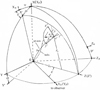 |
Fig. 1. Geometry of the precession model, adopted and generalized from Qian et al. (1991, 2017, 2018). Five coordinate systems are introduced. In the observer’s system (Xn, Yn, Zn), the knot motion is defined by parameters (ϵ, ψ, ω, a, and x) or (ϵ, ψ, ω, r0, and z0). |
We assume that the jet axis locates in the plane (X′,Z′) and is described by a function r0(z0), which is assumed to have a parabolic form, following Asada & Nakamura’s observations of the radio galaxy M87 and modeling results (Asada & Nakamura 2012; Nakamura & Asada 2013; Polko et al. 2010, 2013, 2014)
 (1)
(1)
where a and x are constants. The angle ω between the plane (X, Z) and plane (X′,Z′) represents the precession phase of the jet axis around the Z(Z′)-axis. In the most general case superluminal knots could move helically around the precessing jet axis and thus should be described by the parameters (A, ϕ) in the coordinate system (x′,y′,z′), where the z′-axis is along the tangent to the jet axis and the plane (x′,y′) is perpendicular to the local jet axis. Here ϕ represents the phase of the helical motion and A represents the amplitude. Both are functions of arc-length s0 along the jet axis:
 (2)
(2)
The axial distance z0(=Z) and A(s0) are measured in units of milliarcseconds (mas) and the phases ω and ϕ are measured in units of radians. In this paper we do not consider the helical motion of the superluminal components and thus we assume A ≡ 0 and only consider their motion along the precessing jet axis (parabolic trajectory pattern).
In this simplified case, knots move along the jet axis, and their coordinates (X, Y, Z)≡(Xj, Yj, Zj) and the coordinates of the precessing jet axis (Xj, Yj, Zj) are
 (3)
(3)
 (4)
(4)
 (5)
(5)
When the parameters ϵ, ψ, a, x, and Γ (bulk Lorentz factor of the knot) are set, the kinematics of the knot (projected trajectory, apparent velocity, Doppler factor, and viewing angle as functions of time) can then be calculated. The formulas are described as
![Mathematical equation: $$ \begin{aligned} {X_n}({z_0},{\omega })&={X_j}({z_0},{\omega }){\cos }{\psi }- [{z_0}{\sin }{\epsilon }-{Y_j}({z_0},{\omega }){\cos }{\epsilon }]{\sin }{\psi },\end{aligned} $$](/articles/aa/full_html/2019/01/aa33508-18/aa33508-18-eq6.gif) (6)
(6)
![Mathematical equation: $$ \begin{aligned} {Y_n}({z_0},{\omega })&={X_j}({z_0},{\omega }){\sin }{\psi }+ [{z_0}{\sin }{\epsilon }-{Y_j}{\cos }{\epsilon }]{\cos }{\psi }, \end{aligned} $$](/articles/aa/full_html/2019/01/aa33508-18/aa33508-18-eq7.gif) (7)
(7)
introducing the functions
![Mathematical equation: $$ \begin{aligned} {\Delta }={\arctan \left[\left(\frac{\mathrm{d}X}{\mathrm{d}{z_0}}\right)^2+\left(\frac{\mathrm{d}Y}{\mathrm{d}{z_0}}\right)^2\right]^{\frac{1}{2}}} \end{aligned} $$](/articles/aa/full_html/2019/01/aa33508-18/aa33508-18-eq8.gif) (8)
(8)
and
![Mathematical equation: $$ \begin{aligned}&{{\Delta }_p}={\arctan \left[\frac{\mathrm{d}Y}{\mathrm{d}{z_0}}\right]} ,\end{aligned} $$](/articles/aa/full_html/2019/01/aa33508-18/aa33508-18-eq9.gif) (9)
(9)
![Mathematical equation: $$ \begin{aligned}&{\cos {{\Delta }_s}}={\left[1+\left(\frac{\mathrm{d}X}{\mathrm{d}{z_0}}\right)^2+\left(\frac{\mathrm{d}Y}{\mathrm{d}{z_0}}\right)^2\right]^{-1/2}}. \end{aligned} $$](/articles/aa/full_html/2019/01/aa33508-18/aa33508-18-eq10.gif) (10)
(10)
We can then calculate the viewing angle θ, apparent transverse velocity βa, Doppler factor δ, and the elapsed time T (at which the knot reaches distance z0) as
![Mathematical equation: $$ \begin{aligned}&{\theta }=\arccos [\cos \Delta (\cos \epsilon +\sin \epsilon \tan {{\Delta }_p})] ,\end{aligned} $$](/articles/aa/full_html/2019/01/aa33508-18/aa33508-18-eq11.gif) (11)
(11)
 (12)
(12)
 (13)
(13)
 (14)
(14)
z is redshift, β = v/c, v is the spatial velocity of knot, and Γ = (1 − β2)−1/2 is the Lorentz factor.
We note that in the scenario of the precessing jet nozzle model described above, the precessing common trajectory is defined in the coordinate system (X, Y, Z,) and is described by the parameters a, x, and ω. With respect to the observer’s system (Xn, Yn, Zn) the trajectory is defined by the parameters (a, x, ω, ϵ, ψ). Generally, changes in any parameter or their combination will introduce the change of the trajectory pattern in the observer’s system. In particular, in the following model-fitting of the kinematics of the superluminal components, changes in parameter ψ will be applied to study the knots’ trajectory curvatures in their outer jet regions, while in their innermost jet regions parameter ψ will be assumed to be constant to demonstrate their motion following a precessing common trajectory. In these cases the changes in ψ imply their outer trajectory rotating about the viewing axis Yn. We note that angle ϵ is assumed to be a constant.
It is emphasized here that our precession model is mainly used to fit the innermost trajectory of the knots and their ejection position angles. Due to non-ballistic motions near the core their ejection position angles are quite different from the average position angles measured within ∼1 mas of core separation (e.g., Lister et al. 2013; Chatterjee et al. 2008).
As we have argued, 3C279 may have a double-jet structure and the source kinematics may be explained in terms of a double-jet precession scenario. A sketch is shown in Fig. 2 to describe the assumed double-jet structure that contains two jets designated as jet-A and jet-B. We give the model-fitting results for the superluminal components of jet-A and those of jet-B.
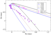 |
Fig. 2. Sketch of the double-jet scenario: the projected cone of the precessing jet-A (northern jet; solid lines) and the projected cone of the precessing jet-B (southern jet; dashed lines). Numbers denote the corresponding precession phases for the trajectories. ω = 6.0 rad and 3.0 rad approximately denote the edges of the cones. Red circles and violet squares are the data points for knots C31 and C7a, respectively. |
In this paper we adopt the concordant cosmological model (ΛCDM model) with Ωm = 0.27, Ωλ = 0.73, and Hubble constant H0 = 70 km s−1 Mpc−1 (Spergel et al. 2003). Thus, for 3C279, z = 0.538, its luminosity distance DL = 3.096 Gpc (Hogg 1999; Pen 1999), and angular distance DA = 1.309 Gpc. Angular scale 1 mas = 6.35 pc and proper motion of 1 mas yr−1 is equivalent to an apparent velocity of 31.81 c, where c is the speed of light.
5. Selection of model parameters
In order to model-fit the kinematics of the superluminal knots in terms of our precessing nozzle model, we need to select two sets of model parameters:
-
Geometric and kinematic parameters, which include parameters ϵ and ψ defining the orientation of the jet axis; parameters a and x defining the precessing common parabolic trajectory; and the Lorentz factor for each of the knots. Based on the observed kinematic features of the knots we can deduce a preliminary set of these parameters. For example, if the viewing angle of the jet is given, then (i) the shape of the precessing common trajectory (parameters a and x) can be roughly determined from the observed shapes of the knots’ tracks; (ii) from the observed (approximate) symmetric distribution of the trajectories of the knots, the position of the jet axis and its spatial orientation (ψ) can be estimated; and (iii) the Lorentz factors of the knots can be estimated from their observed apparent velocities. The selection of these parameters is not unique, and largely depends on the viewing angle of the jet (or parameter ϵ). They are selected through trial model-fittings of the kinematics of the knots, using the formalism described in Sect. 4. Since different viewing angles selected for the precession axis would cause different projection effects and thus result in different geometric and kinematic parameters, we should choose an appropriate value for parameter ϵ. In this paper we take ϵ = 0.0230 rad = 1.32°, which is consistent with the values obtained by VLBI measurements (Hovatta et al. 2009; Jorstad & Marscher 2005).
-
Parameters that describe the kinematic behavior of the knots changing with time: the ejection times t0 of the knots and the precession period Tp. Although the geometric and kinematic parameters are not uniquely selected, the model ejection times t0 and the precession period Tp are strictly constrained by the observed ejection times and the observed distribution of the trajectories. We can select the second set of model parameters as follows. The observed ejection times derived from the VLBI measurements can be used as the approximate values for the model ejection times. Usually, the observed ejection time of a knot is derived by extrapolating its core separation to zero by linear regression. If trajectories are non-radial, this method could induce significant errors. The precession period can be estimated from the distribution of the knot’s trajectory and their ejection times. So we can also derive these parameters through trial model-fittings.
6. Model-fitting of jet-A kinematics
Through trial model-fittings we found that jet-A ejected 18 superluminal components (C3, C4, C7a, C8–C16, C21–C26), which can be consistently model-fitted in terms of the precession nozzle scenario with a precession period of 25 yr. The model parameters have been selected and are shown in Table 1. The ejection time t0 of the knots is calculated with the following formula,
Model parameters of the precessing nozzle scenario for jet-A (northern jet).
 (15)
(15)
where 1996.89 is the ejection epoch of knot C9 having precession phase 4.15 rad. The precession period Tp = 25 yr.
6.1. Modeling results for jet-A
The model parameters for jet-A are are given in Table 1: Jet orientation parameters, ϵ = 0.0230 rad (=1.32°) and ψ = 0.50 rad (=28.65°); parameters defining the common parabolic trajectory shape, a = 0.0342 [mas]0.75 and x = 0.25; precession period, Tp = 25 yr.
The overall distribution of trajectory of the knots is shown in Fig. 3. The modeled parameters (precession phase ω, ejection epoch t0, range of modeled bulk Lorentz factor Γ) and the VLBI measured ejection epoch t0, VLBI are summarized in Table 2. We describe the model-fitting results for each of the knots, including the fits to the trajectory, core separation versus time, modeled apparent velocity, viewing angle, modeled bulk Lorentz factor, and Doppler factor, which are shown in Figs. 4–7 and A.1–A.7.
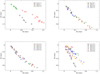 |
Fig. 3. Distribution of the knots’ trajectories for (northern) jet-A, shown separately in four subsets: (C3, C4, C7a), (C8–C11), (C12–C16), (C21–C26). The coordinates of the four panels have been chosen in proportional scales for easy comparison of the relative position angles of these trajectories. |
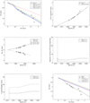 |
Fig. 4. Model-fitting results of the kinematics for knot C3 including trajectory, core separation vs. time, apparent velocity, viewing angle, Lorentz factor, and Doppler factor. Upper left panel: the red dashed line denotes the modeled precessing common trajectory and the entire observed trajectory is model-fitted by the black dashed line. The green and blue lines represent the fitting model trajectories calculated for precession phases ω ± 0.63 rad. Bottom right panel: the green and blue lines represent the precessing common parabolic trajectories calculated for precession phases ω ± 0.63 rad. |
Precessing nozzle model for jet-A with a period of 25 yr.
We use two criteria to judge the validity of our approach to the model-fitting of the source kinematics: (1) In the model-fitting of the knot’s trajectory, we show two additional fitting model trajectories calculated for precession phases ω + 0.63 rad and ω − 0.63 rad (corresponding to ejection times t0 + 2.5 yr and t0 − 2.5 yr). We found for all the knots that most of their observation data points are located within the position angle range defined by the two trajectories, indicating that the precession period was determined within an uncertainty of ±2.5 yr. (2) In the model-fitting of the knot’s trajectory, we also show two additional precessing common trajectories calculated for precession phases ω + 0.63 rad and ω − 0.63 rad. For some knots we found that a number of their observation data points are located within the position angle range defined by the two trajectories, indicating their innermost trajectory have been observed to follow the precessing common parabolic trajectory. These knots are designated by the symbol “+” in Table 3. For for some knots, however, there are no observation data points located within the position angle range defined by the two precessing common trajectories, indicating that more observations are needed to confirm whether their innermost trajectory follows the precessing common parabolic trajectory. These knots will be designated by the symbol “–” in Table 3.
Jet-A: core separations (rn) and corresponding axial distances (Z) within which the knots move along the precessing common trajectory.
It is noted here that (i) in the figure panels for model-fitting of the knots’ trajectories the black lines denote the modeled trajectory for ejection epoch t0 fitting the observed trajectory, and the red lines denote the corresponding precessing common trajectory. These two trajectories only coincide within certain separations, implying curvatures of the observed trajectories in the outer jet regions; (ii) since we assume that the precessing common trajectory has a parabolic form and we take trajectory curvature in outer jet regions into consideration, the motion of the knots needs to be modeled as accelerated or decelerated along the trajectories (modeled Lorentz factor changes along the trajectory), leading to acceleration or deceleration of the apparent motion; (iii) the modeled viewing angle of a knot also changes along the trajectory, and changes very rapidly at separations near the core; and (iv) the modeled apparent velocity usually changes along the trajectory. This feature of the modeled velocity should be kept in mind when comparing it with the VLBI measured velocity: VLBI measurements usually give average values for observed apparent velocities within certain core separations (e.g., within 1 mas; Chatterjee et al. 2008).
6.1.1. Knot C3
The model-fitting results are shown in Fig. 4.
Modeled ejection epoch t0 = 1971.60, precession phase ω = 10.51 rad (=2π + 4.23). Its innermost trajectory within core separation 0.40 mas (corresponding axial distance Z = 15 mas = 95.3 pc) is modeled to follow the precessing common parabolic trajectory, and its inner kinematics can be explained in terms of the precessing nozzle model (ψ = 0.50 rad; the red dashed line in the upper left panel), but no observation data is available to confirm this. Its outer trajectory (rn > 0.40 mas) can be interpreted by introducing trajectory curvatures defined by changes in ψ: for Z = 15 − 32 mas ψ(rad)=0.5 + 0.25(Z − 15)/(32 − 15); for Z = 32 − 90 mas ψ(rad)=0.75 − 0.05(Z − 32)/(90 − 32); and for Z > 90 mas ψ = 0.70 rad. The model of the entire trajectory is shown by the black dashed line.
The motion is required to be modeled as accelerated: for Z < 32 mas Γ = 8.5; for Z = 32 − 90 mas Γ = 8.5 + 2.5(Z − 32)/(90 − 32); and for Z > 90 mas Γ = 11.0. The modeled apparent velocity is consistent with the VLBI measured value 3.8 ± 0.6 c (Unwin et al. 1989).
6.1.2. Knot C4
The model-fitting results are shown in Fig. 5.
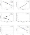 |
Fig. 5. Model-fitting results of the kinematic features for knot C4 including trajectory, core separation, coordinates, apparent velocity, viewing angle, Lorentz factor, and Doppler factor. The entire observed trajectory (prior to 1998.2) can be approximately model-fitted to follow the precessing common trajectory (red dashed line). Upper left panel: the green and blue lines represent the fitting model trajectories calculated for precession phases ω ± 0.63 rad. Bottom right panel: the green and blue lines represent the precessing common parabolic trajectories calculated for precession phases ω ± 0.63 rad. |
Modeled ejection epoch t0 = 1984.68, precession phase ω = 7.22 rad (=2π + 0.94), bulk Lorentz factor Γ = const. = 14.3. Within core separation rn < 0.85 mas (corresponding axial distance Z = 40 mas = 254 pc) the knot can be modeled to follow the precessing common parabolic trajectory (ψ = 0.50 rad; red dashed line in the upper left panel). Beyond rn > 0.85 mas its trajectory can be interpreted by introducing slight curvatures: for Z = 40 − 80 mas ψ(rad)=0.5 − 0.05(Z − 40)/(80 − 40); for Z > 80 mas ψ = 0.45 rad. The model of the entire trajectory is shown by the black dashed line in the upper left panel.
This knot is a very good example; its entire observed trajectory (prior to 1998.2) can be approximately fitted in terms of the precessing nozzle model; that is, knot C4 almost follows the precessing common parabolic trajectory, extending to the axial distance Z = 254 pc (core separation rn = 0.85 mas).
The modeled apparent velocity is well consistent with the VLBI measured average value 7.9 ± 0.6 c (Homan et al. 2003) and 7.5 ± 0.2 c (Wehrle et al. 2001).
In the upper left panel of Fig. 4, the green and blue lines represent the fitting model trajectories calculated for precession phases ω ± 0.63 rad (corresponding to ejection times t0 ± 2.5 yr) and most of the data points are within the position angle range defined by the two trajectories, indicating that the precession period was determined within an uncertainty of ± 2.5 yr. In the bottom right panel, the green and blue lines represent the precessing common trajectories calculated for precession phases ω ± 0.63 rad; a number of the data points are within the position angle range defined by the two trajectories, indicating that its innermost trajectory has been observed to follow the precessing common parabolic trajectory. Thus, knot C4 is designated by symbol “+” in Table 3.
6.1.3. Knot C7a
The model-fitting results are shown in Fig. 6.
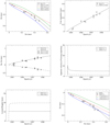 |
Fig. 6. Model-fitting results of the kinematics for knot C7a including trajectory, core separation, coordinates, apparent velocity, viewing angle, Lorentz factor, and Doppler factor. Upper left panel: the green and blue lines represent the fitting model trajectories calculated for precession phases ω ± 0.63 rad. The entire observed trajectory is well fitted (black dashed line) and all the data points are within the position angle range defined by the two lines, indicating that the precession period was determined within an uncertainty of ± 2.5 yr. Bottom right panel: the green and blue lines represent the precessing common parabolic trajectories calculated for precession phases ω ± 0.63 rad. Most of the data points are within the position angle range defined by the two lines, indicating that its innermost trajectory following the precessing common trajectory has been observed and knot C7 is marked by symbol “+” in Table 3. |
Modeled ejection epoch t0 = 1994.67, precession phase ω = 4.71 rad, Lorentz factor Γ = const. = 10.5. Within core separation rn < 0.24 mas (corresponding axial distance Z = 8 mas = 50.8 pc) the knot is modeled to follow the precessing common trajectory (ψ = 0.50 rad; red dashed line in the upper left panel) and its kinematics can be well explained in terms of the precessing nozzle model. Beyond rn = 0.24 mas its trajectory can be fitted by introducing changes in parameter ψ: for Z = 8 − 30 mas ψ(rad)=0.5 + 0.13(Z − 8)/(30 − 8); for Z > 30 mas ψ = 0.63 rad. The model of the entire trajectory is shown by the black dashed line.
The modeled apparent velocity is consistent with the VLBI measured value 5.0 ± 0.3 c (Homan et al. 2003; Wehrle et al. 2001; Jorstad et al. 2004).
In the upper left panel of Fig. 6, the green and blue lines represent the fitting model trajectories calculated for precession phases ω ± 0.63 rad and all the data points are within the position angle range defined by the two trajectories, indicating that the precession period was determined within an uncertainty of ±2.5 yr. In the bottom right panel, the green and blue lines represent the precessing common trajectories calculated for precession phases ω ± 0.63 rad and most of the data points are within the position angle range defined by the two trajectories, indicating that its innermost trajectory was observed to follow the precessing common parabolic trajectory. Knot C7 is marked by the symbol “+” in Table 3.
6.1.4. Knot C8
The model-fitting results are shown in Fig. 7.
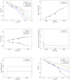 |
Fig. 7. Model-fitting results of the kinematics for knot C8 including trajectory, core separation, coordinates, apparent velocity, viewing angle, Lorentz factor, and Doppler factor. Upper left panel: the green and blue lines represent the fitting model trajectories calculated for precession phases ω ± 0.63 rad. The entire observed trajectory is well fitted (black dashed line) and the observation data points are all within the position angle range defined by the two lines, indicating that the precessing period was determined within an uncertainty of ± 2.5 yr. Bottom right panel: the green and blue lines represent the precessing common parabolic trajectories calculated for precession phases ω ± 0.63 rad and a number of the observation data points are within the position angle range defined by the two lines, indicating that its innermost trajectory following the precessing common trajectory has been observed and knot C8 is marked by symbol “+” in Table 3. |
Modeled ejection epoch t0 = 1995.70, precession phase ω = 4.45 rad, Lorentz factor Γ = const. = 10.3. The observed trajectory within core separation rn < 0.072 mas (corresponding axial distance Z = 1.5 mas = 9.53 pc) is modeled to follow the precessing common trajectory (ψ = 0.50 rad; red dashed line in the upper left panel of Fig. 7) and its kinematics can be understood in terms of the precessing nozzle model. Beyond rn = 0.072 mas its trajectory can be explained by introducing changes in parameter ψ: for Z = 1.5 − 3.0 ψ(rad)=0.5 + 0.15(Z − 1.5)/(3 − 1.5); for Z = 3 − 7 mas ψ(rad)=0.65 − 0.07(Z − 3)/(7 − 3); for Z = 7 − 15 mas ψ(rad)=0.58 + 0.20(Z − 7)/(15 − 7); for Z > 15 mas ψ = 0.78 rad. The entire observed trajectory can be well fitted by the model (black dashed line in the upper left panel).
The modeled apparent velocity is consistent with the VLBI measured value 5.4 ± 0.7 c (Chatterjee et al. 2008).
In the upper left panel of Fig. 7, the green and blue lines represent the fitting model trajectories calculated for precession phases ω ± 0.63 rad and all the data points are within the position angle range defined by the two trajectories, indicating that the precession period was determined within an uncertainty of ±2.5 yr. In the bottom right panel, the green and blue lines represent the precessing common trajectories calculated for precession phases ω ± 0.63 rad and a number of the data points are within the position angle range defined by the two trajectories, indicating that its innermost trajectory was observed to follow the precessing common parabolic trajectory. Knot C8 is designated by symbol “+” in Table 3.
Knots C4, C7a, and C8 have similar kinematic features, verifying the 25 yr precession period with their innermost trajectories following the precessing common parabolic trajectory. More model-fitting results are shown in Figs. A.1–A.7, which demonstrate that the kinematic features for more knots can be well fitted in terms of the precessing nozzle model.
6.1.5. Knot C9
The model-fitting results are shown in Fig. A.1 (first 6 panels, from top left to bottom right).
Modeled ejection epoch t0 = 1996.89, precession phase ω = 4.15 rad, Lorentz factor Γ = const. = 17.5. Within core separation rn = 0.083 rad (corresponding axial distance Z = 2 mas = 12.7 pc) its motion is modeled to follow the precessing common trajectory (ψ = 0.50 rad; red dashed line in the first panel of Fig. A.1) and its kinematics can be interpreted in terms of the precessing nozzle model. Beyond rn = 0.083 mas its outer trajectory (from rn = 0.2 mas–2 mas) can be well fitted by introducing changes in parameter ψ: for Z = 2 − 8 mas ψ(rad)=0.5 + 0.2(Z − 2)/(8 − 2); for Z = 8 − 80 mas ψ(rad)=0.70 − 0.15(Z − 8)/(80 − 8); for Z > 80 mas ψ = 0.55 rad. The entire modeled trajectory is shown by the black dashed line.
The modeled apparent velocity is consistent with the VLBI measured value 12.9 ± 0.3 c (Chatterjee et al. 2008).
6.1.6. Knot C10
The model-fitting results are shown in Fig. A.1 (last six panels).
Modeled ejection epoch t0 = 1997.24, precession phase ω = 4.06 rad, Lorentz factor Γ = const. = 16.0. Within core separation rn = 0.082 mas (corresponding axial distance Z = 2 mas = 12.7 pc) its observed trajectory can be modeled to follow the precessing common trajectory (ψ = 0.50 rad; red dashed line in the 7th panel of Fig. A.1) and its kinematics can be interpreted in terms of the precessing nozzle model. Beyond this separation its outer trajectory can be fitted by introducing changes in parameter ψ (or trajectory curvatures): for Z = 2 − 15 mas ψ(rad)=0.5 + 0.25(Z − 2)/(15 − 2); for Z = 15 − 65 mas ψ = 0.75 − 0.35(Z − 15)/(65 − 15); for Z > 65 mas ψ = 0.40 rad. The entire observed trajectory is well fitted by the model (black dashed line).
The modeled apparent velocity is consistent with the VLBI measured average value 9.9 ± 0.5 c (Chatterjee et al. 2008).
6.1.7. Knot C11
The model-fitting results are shown in Fig. A.2 (first 6 panels, from top left to bottom right).
Modeled ejection epoch t0 = 1997.59, precession phase ω = 3.974 rad, Lorentz factor Γ = const. = 16.0. Within core separation rn = 0.067 mas (corresponding axial distance Z = 2 mas = 12.7 pc) its trajectory can be modeled to follow the precessing common trajectory (ψ = 0.50 rad; red dashed line in the first panel of Fig. A.2) and its kinematics can be interpreted in terms of the precessing jet model. Beyond this separation its outer trajectory can be interpreted by introducing changes in parameter ψ (trajectory curvatures): for Z = 2 − 9 mas ψ(rad)=0.5 + 0.3(Z − 2)/(9 − 2); for Z = 9 − 40ψ(rad)=0.8 − 0.45(Z − 9)/(40 − 9); for Z > 40 mas ψ = 0.35 rad. The entire modeled trajectory is shown by the black dashed line.
The modeled apparent velocity is consistent with the VLBI measured average value 10.1 ± 1.2 c (Chatterjee et al. 2008).
6.1.8. Knot C12
The model-fitting results are shown in Fig. A.2 (last six panels).
Modeled ejection epoch t0 = 1998.46, precession phase ω = 3.755 rad. Its inner path within core separation 0.05 mas (corresponding axial distance Z = 1.0 mas = 6.4 pc) follows the precessing common trajectory (ψ = 0.5 rad) and its inner kinematics can be well explained in terms of the precessing nozzle model. However, for explaining its outer path (rn > 0.05 mas) changes in the parameter ψ are required: for Z = 1 − 5 mas ψ(rad)=0.5 + 0.05(Z − 1)/(5 − 1); for Z > 5 mas ψ = 0.55 rad. For explaining its separation versus time, a deceleration of its motion is required: for Z ≤ 1.0 mas Γ = 21; for Z = 1 − 5 mas Γ = 21 − 2(Z − 1)/(5 − 1); for Z > 5 mas Γ = 19.
The modeled apparent velocity is consistent with the VLBI measured average value 16.9 ± 0.4 c (Chatterjee et al. 2008).
As shown in the last panel of Fig. A.2 its innermost trajectory has been observed to follow the precessing common parabolic trajectory. Knot C12 is designated by symbol “+” in Table 3.
6.1.9. Knot C13
The model-fitting results are shown in Fig. A.3 (first 6 panels, from top left to bottom right).
Modeled ejection epoch t0 = 1998.88, precession phase ω(rad)=3.65. Its inner path within core separation rn = 0.15 mas (axial distance Z = 5 mas = 32 pc) follows the precessing common trajectory (ψ = 0.5 rad) and its inner kinematics can be explained in terms of the precessing nozzle model. However, for explaining its outer path (rn > 0.15 mas) changes in ψ are required: for Z(mas)=5 − 20ψ = 0.5 + 0.1(Z − 5)/(20 − 5); for Z > 20 mas ψ = 0.60 rad. For explaining its separation versus time, an acceleration of its motion is required: for Z ≤ 5 mas Γ = 17; for Z = 5 − 10 mas Γ = 17 + 3.5(Z − 5)/(10 − 5); for Z > 10 mas Γ = const. = 20.5.
The modeled apparent velocity is consistent with the VLBI measured average value 16.4 ± 0.5 c (Chatterjee et al. 2008).
As shown in the 6th panel of Fig. A.3, its innermost trajectory has been observed to follow the precessing common parabolic trajectory and knot C13 is designated by symbol “+” in Table 3.
6.1.10. Knot C14
The model-fitting results are shown in Fig. A.3 (last six panels).
Modeled ejection epoch t0 = 1999.40, precession phase ω = 3.52 rad. Its inner path within core separation rn = 0.14 mas (axial distance Z = 5 mas = 32 pc) follows the precessing common trajectory (ψ = 0.5 rad) and its inner kinematics can be interpreted in terms of the precessing nozzle model. However, for explaining its outer path (rn > 0.14 mas) changes in ψ are introduced: for Z = 5 − 13 mas ψ(rad)=0.5 + 0.12(Z − 5)/(13 − 5); for Z > 13 mas ψ = 0.62 rad. In order to explain its separation versus time, an acceleration of its motion is required: for Z ≤ 5 mas Γ = 17.5; for Z = 5 − 13 mas Γ = 17.5 + 5.5(Z − 5)/(13 − 5); for Z > 13 mas Γ = 23.
The modeled apparent velocity is consistent with the VLBI measured average value 18.2 ± 0.7 c (Chatterjee et al. 2008).
As shown in the last panel of Fig. A.3, its innermost trajectory has been observed to follow the precessing common parabolic trajectory and knot C14 is designated by symbol “+” in Table 3.
6.1.11. Knot C15
The model-fitting results are shown in Fig. A.4 (first 6 panels, from top left to bottom right).
Modeled ejection epoch t0 = 1999.75, precessing phase ω = 3.43 rad. Its inner path within core separation 0.14 mas (axial distance Z = 5 mas = 32 pc) follows the precessing common trajectory (ψ = 0.5 rad) and its inner kinematics can be interpreted in terms of the precessing nozzle model. However, in order to interpret its outer path (rn > 0.14 mas) changes in the parameter ψ are introduced: for Z = 5 − 20 mas ψ(rad)=0.5 + 0.16(Z − 5)/(20 − 5); for Z > 20 mas ψ = 0.66 rad. To explain its separation versus time, a uniform motion is assumed: Γ = const. = 19.
The modeled apparent velocity is consistent with the VLBI measured average value 17.2 ± 2.3 c (Chatterjee et al. 2008).
As shown in the 6th panel of Fig. A.4, its innermost trajectory has been observed to follow the precessing common parabolic trajectory and knot C15 is designated by symbol “+” in Table 3.
6.1.12. Knot C16
The model-fitting results are shown in Fig. A.4 (last six panels).
Modeled ejection epoch t0 = 2000.17, precession phase ω = 3.33 rad. Its inner path within core separation 0.13 mas (axial distance Z = 5 mas = 32 pc) follows the precessing common trajectory (ψ = 0.50 rad) and its inner kinematics can be interpreted in terms of the precessing nozzle model. However, for explaining its outer path (rn > 0.13 mas) changes in ψ (or trajectory curvatures) are introduced: for Z = 5 − 12 mas ψ(rad)=0.5 + 0.2(Z − 5)/(12 − 5); for Z > 12 mas ψ = 0.70 rad. In order to fit its separation versus time, an acceleration of its motion is required: for Z ≤ 5 mas Γ = 17; for Z = 5 − 12 mas Γ = 17 + 8(Z − 5)/(12 − 5); for Z > 12 mas Γ = 25.
The modeled apparent velocity is consistent with the VLBI measured average value 16.9 ± 3.5 c (Chatterjee et al. 2008).
As shown in the last panel of Fig. A.4, its innermost trajectory has been observed to follow the precessing common parabolic trajectory and knot C16 is designated by symbol “+” in Table 3.
We note that the kinematics of knots C13, C14, C15, and C16 are similar: their trajectory curvatures occur at similar separations of ∼0.14 mas (corresponding axial distance Z ∼ 32 pc).
6.1.13. Knot C21
The model-fitting results are shown in Fig. A.5 (first 6 panels, from top left to bottom right).
Modeled ejection epoch t0 = 2004.65, precession phase ω = 2.20 rad. Its inner path within core separation 0.03 mas (axial distance Z = 2 mas = 12.7 pc) can be understood to follow the precessing common trajectory (ψ = 0.50 rad) and its inner kinematics can be interpreted in terms of the precessing nozzle model. However, for explaining the observed outer path (rn > 0.03 mas) changes in parameter ψ (or trajectory curvatures) are introduced: for Z = 2 − 6 mas ψ(rad)=0.50 + 0.40(Z − 2)/(6 − −2); for Z > 6 mas ψ = 0.90 rad. To explain its separation versus time, a deceleration of its motion is required: for Z ≤ 1.5 mas Γ = 26; for Z = 1.5 − 2.0 mas Γ = 26 − 5(Z − 1.5)/(2 − 1.5); for Z > 2 mas Γ = 21.
The modeled apparent velocity is consistent with the VLBI measured average value 16.7 ± 0.3 c (Chatterjee et al. 2008).
6.1.14. Knot C22
The model-fitting results are shown in Fig. A.5 (last six panels).
Modeled ejection epoch t0 = 2005.08, precession phase ω = 2.092 rad. Its inner path within core separation rn = 0.04 mas (axial distance Z = 3 mas = 19 pc) can be understood to follow the precessing common trajectory (ψ = 0.5 rad) and its inner kinematics could be explained in terms of the precessing nozzle model. However, for explaining its observed outer trajectory changes in parameter ψ (or trajectory curvatures) are introduced: for Z = 3 − 12 mas ψ(rad)=0.50 − 0.32(Z − 3)/(12 − 3); for Z > 12 mas ψ = 0.18 rad. In order to explain its core separation versus time, a deceleration of its motion is required: for Z ≤ 1.5 mas Γ = 18; for Z = 1.5 − 2.5 mas Γ = 18 − 2.3(Z − 1.5)/(2.5 − 1.5); for Z > 3 mas Γ = 15.7.
The modeled apparent velocity is approximately consistent with the VLBI measured average value 12.4 ± 1.2 c (Chatterjee et al. 2008).
As shown in the last panel of Fig. A.5, its innermost trajectory has been observed to follow the precessing common parabolic trajectory and knot C22 is designated by symbol “+” in Table 3.
6.1.15. Knot C23
The model-fitting results are shown in Fig. A.6 (first 6 panels, from top left to bottom right).
Modeled ejection epoch t0 = 2006.26, precession phase ω = 1.80 rad. Its inner trajectory within core separation rn = 0.17 mas (Z = 10 mas = 64 pc) follows the precessing common trajectory pattern (ψ = 0.50 rad). Its outer trajectory is curved and changes in parameter ψ (or trajectory curvatures) are introduced: for Z = 10 − 30 mas ψ(rad)=0.50 − 0.05(Z − 10)/(30 − 10); for Z > 30 mas ψ = 0.45 rad. Its motion is assumed to be decelerated: for Z ≤ 1.5 mas Γ = 30; for Z = 1.5 − 3.0 Γ = 30 − 8(Z − 1.5)/(3.0 − 1.5); for Z > 30 Γ = 22.
The modeled apparent velocity is consistent with the VLBI measured average value 16.5 ± 2.3 c (Chatterjee et al. 2008; Larionov et al. 2008).
As shown in the 6th panel of Fig. A.6, its innermost trajectory has been observed to closely follow the precessing common parabolic trajectory and knot C23 is designated by symbol “+” in Table 3.
6.1.16. Knot C24
The model-fitting results are shown in Fig. A.6 (last six panels).
Modeled ejection epoch t0 = 2006.88, precession phase ω = 1.64 rad. Its inner trajectory within core separation rn ≤ 0.28 mas (axial distance Z = 15 mas = 95.3 pc) follows the precessing common trajectory (ψ = 0.5 rad) and its inner kinematics can be well fitted by the precessing nozzle model. However, in the outer trajectory region (core separation rn > 0.28 mas, Z > 15 mas) trajectory deviations from the precessing common trajectory or trajectory curvatures are introduced: for Z = 15 − 30 mas ψ(rad)=0.5 + 0.2(Z − 15)/(30 − 15); for 30–65 ψ(rad)=0.7 − 0.3(Z − 30)/(65 − 30); for Z > 65 mas ψ = 0.4 rad. Deceleration of its motion is assumed to fit its separation versus time: for Z ≤ 15 mas Γ = 24; for Z = 15 − 30 mas Γ = 24 − 10(Z − 15)/(30 − 15); Z > 30 mas Γ = 14.
We note that the observed trajectory of knot C24 is a good model-fitting example, which shows that the observation data points (within core separation rn ≃ 0.4 mas) cluster around the precessing common trajectory (the red line in the last panel of Fig. A.6) and its kinematic behavior (ejection epoch, ejection position angle, and its initial trajectory) closely follows the precessing jet nozzle model.
The modeled apparent velocity varies with time prominently, but is consistent with the VLBI measured average value 14.7 ± 0.9 c (2007–2008; Larionov et al. 2008).
We note that both knots C23 and C24 are very good examples, for which a great number of data points are clustered around the precessing common trajectory, showing that their innermost trajectories have been firmly observed to follow the precessing common parabolic trajectory pattern.
6.1.17. Knot C25
The model-fitting results are shown in Fig. A.7 (first 6 panels, from top left to bottom right).
Modeled ejection epoch t0 = 2007.09, precession phase ω = 1.590 rad. Its inner trajectory within core separation rn = 0.17 mas (axial distance Z ≤ 10 mas = 64 pc) follows the precessing common trajectory (ψ = 0.5 rad) and its inner kinematics can be well fitted by the precessing nozzle model. However, in its outer trajectory region (Z > 10 mas) trajectory deviations from the precessing common trajectory or trajectory curvatures are introduced: for Z = 10 − 30 mas ψ(rad)=0.50 + 0.25(Z − 10)/(30 − 10); for Z = 30 − 65 mas ψ(rad)=0.75 − −0.20(Z − 30)/(65 − 30); for Z > 65 mas ψ = 0.55 rad. For explaining its core separation versus time, an acceleration of its motion is assumed: for Z ≤ 10 mas Γ = 16.0; for Z = 10 − 30 mas Γ = 16 + 3(Z − 10)/(30 − 10); for Z > 30 Γ = 19.
The modeled apparent velocity is consistent with the VLBI measured average value 12.3 ± 0.43 c (Jorstad et al. 2017).
Knot C25 is another good example, showing that its innermost trajectory has been firmly observed to follow the precessing common parabolic trajectory pattern (see 6th panel of Fig. A.7).
6.1.18. Knot C26
The model-fitting results are shown in Fig. A.7 (last six panels).
Modeled ejection epoch t0 = 2007.10, precession phase ω = 1.587 rad. Its inner trajectory within core separation 0.13 mas (axial distance Z = 8 mas = 51 pc) follows the precessing common trajectory (ψ = 0.5 rad) and its inner kinematics can be understood in terms of the precessing nozzle model (but no observation points there). Its outer trajectory region (rn > 0.13 mas or Z > 8 mas) trajectory deviations from the common trajectory or trajectory curvatures are introduced: for Z = 8 − 18 mas ψ(rad)=0.50 + 0.43(Z − 8)/(18 − 8); for Z > 18 mas ψ = 0.93 rad. For explaining the core separation versus time, the Lorentz factor is assumed to be constant: Γ = 11.5.
The modeled apparent velocity is consistent with the VLBI measured average value 4.87 ± 0.48 c (Jorstad et al. 2017).
We note that the data on knots C25 and C26, which were not available before, are newly included here (Qian 2013). It can be seen that for knot C25 a number of data points (within core separation rn = 0.17 mas) are clustered around the precessing common trajectory (the red line in the 6th panel of Fig. A.7), and its kinematic behavior (ejection epoch, ejection position angle, and the initial trajectory) is observed to be consistent with that predicted by the model, and thus really help to verify our precessing nozzle model.
6.2. Brief summary of jet-A
We have presented the model-fitting results of the kinematic features of the superluminal components (18 in total) of jet-A. The innermost kinematics observed for most of the knots (trajectory, core separation, and apparent velocity) can be consistently well fitted (or simulated) in terms of the precessing nozzle model with a precession period 25 ± 2.5 yr. Their Lorentz factor, Doppler factor, and viewing angle are also derived (see Table 2 and explanations for individual knots in Sect. 6.1). In Table 3 the range of distances from the core, within which their observed trajectories can be fitted by the precessing common trajectory, are summarized.
The chief results can be summarized as follows:
-
(1)
As shown in Figs. 4–7 and A.1–A.7, most of the observation data points are within the position angle range defined by the two modeled trajectories calculated for t0 ± 2.5 yr (the green and blue lines) and thus the precession period was determined within an uncertainty of ∼ ± 2.5 yr (∼10% of the period);
-
(2)
As shown in Table 3, 11 knots designated with symbol “+” (occupying ∼70%) are observed having their initial paths along the precessing common trajectory: knots C4, C7a, C12, C13, C14, C15, C16, C23, C24, and C25 are good examples. Knot C4 is observed to have the longest core separation (∼40 mas = 250 pc) following the precessing common trajectory. These consistent modeling results may argue strongly for the validity of the precession nozzle scenario for jet-A;
-
(3)
The modeled trajectory curvatures occur at very different core separations from 0.03 mas to 0.85 mas (or radial distance Z from 6.4 pc to 250 pc). This indicates that the knots have various trajectory shapes and a very complex trajectory distribution. This explains why the regular precession behavior of 3C279 is so difficult to be searched and can only be found through model simulations by decomposing the complex kinematic ingredients;
-
(4)
In a few cases the modeled Lorentz factors and apparent velocities vary along the trajectories. For the entire group of knots of jet-A, the modeled Lorentz factor ranges from 9 to 25, the modeled Doppler factor from 20 to 35, and the modeled viewing angle from ∼1.22° to ∼1.48°; all these values are generally consistent with those obtained from the VLBI measurements (Lister et al. 2013; Jorstad et al. 2017, 2004; Jorstad & Marscher 2005; Homan et al. 2003; Lister & Marscher 1997; Chatterjee et al. 2008; Larionov et al. 2008; Wehrle et al. 2001).
7. Model-fitting of jet-B kinematics
In the last section we discussed the model-fitting results of the kinematics for jet-A, containing 18 superluminal components (C3, C4, C7a, C8–C16, and C21–C26). As we argued in Sect. 2, to understand the kinematics in 3C279 on parsec-scales, a double-jet scenario may be needed. We designate the second jet as jet-B, which precesses with the same precession period of 25 yr and ejects superluminal components. Here we present the model-fitting results of the kinematics for the knots of this second jet.
The superluminal knots of jet-B are divided into two groups, group-1 and group-2: Group-1 contains seven superluminal components (C5a, C6, C7, and C17–C20), and group-2 contains six knots (C27–C32) which were all measured after 2008 and will be mainly used to test the precessing jet nozzle model for jet-B and the entire double-jet scenario.
The model parameters of the precessing nozzle model for jet-B are chosen as follows (for both groups). Parameters for defining the orientation of jet-B: ϵ = 1.32 ° =0.0230 rad and ψ = 1.15 rad = 65.90°; parameters for the parabolic trajectory shape: a = 0.0670[mas]0.75 and x = 0.25; precession period Tp = 25 yr. They are listed in Table 4. The value of ψ for jet-B is different from that for jet-A, indicating its different orientation in space (Fig. 2). The value of a is also different from that for jet-A, denoting its different parabolic shape of the precessing common trajectory.
Model parameters of the precessing nozzle scenario for jet-B.
The ejection epochs of the knots are calculated from their precession phases,
 (16)
(16)
where 1993.34 is the ejection epoch for knot C7 having a precession phase ω = 7.00 rad and Tp = 25 yr, the precession period of the second jet.
The trajectory distribution of the knots are shown in four panels of Fig. 8: for knots C5a–C7, C17–C20, C27–C29, and C30–C32. They reveal some trends of clustering of the knot trajectories.
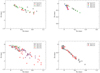 |
Fig. 8. Trajectory distribution of the knots of jet-B, shown in four subsets: (C5a–C7), (C17–C20), (C27–C30), and (C31–C32), revealing some trends of the clustering of their trajectory and ejection direction. The coordinates in the four panels have similar scales for easy inspection of the relative distribution of these trajectories. |
The modeled ejection epoch t0, corresponding precession phase ω and Lorentz factor Γ, and the VLBI measured ejection epochs t0, VLBI are summarized in Table 5.
Model parameters of the precessing nozzle model with a period of 25 yr for jet-B.
We describe the model-fitting results for each knot, including the fits to the trajectory, core separation versus time, and apparent velocity. The modeled viewing angle, Lorentz factor, and Doppler factor are also given. The fitting results are shown in Figs. 9–11 and B.1–B.7.
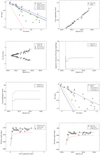 |
Fig. 9. Model-fitting results of the kinematics for knot C30. In the bottom panels the modeled relations between its observed position angle vs. core separation (left) and vs. time (right) are shown. The black lines denote the fitting model and the red lines indicate the precessing nozzle model. The black line and the red line coincide only at their initial parts near the core due to the trajectory curvatures in the outer jet regions. We note that the first data point (Xn = −0.46 mas, Zn = −0.074 mas) is correctly located on the precessing common parabolic trajectory. |
As before, we will use two criteria to judge the validity of our approach to the model-fitting of the source kinematics: (1) in the model-fitting of the knot’s trajectory we show two additional fitting model trajectories calculated for precession phases ω + 0.63 rad and ω − 0.63 rad (corresponding to ejection times t0 + 2.5 yr and t0 − 2.5 yr). We found for all the knots that most of their observation data points are located within the position angle range defined by the two trajectories, indicating that the precession period was determined within an uncertainty of ±2.5 yr; (2) in the model-fitting of the knot’s trajectory we also show two additional precessing common trajectories calculated for precession phases ω + 0.63 rad and ω − 0.63 rad. We found for some knots that a number of observation data points are located within the position angle range defined by the two trajectories, indicating their innermost trajectory has been observed to follow the precessing common parabolic trajectory. These knots will be designated by the symbol “+” in Table 6. However, for some knots there are no data points located within the position angle range defined by the two trajectories, indicating more observations needed to confirm whether their innermost trajectory following the precessing common trajectory. These knots will be designated by the symbol “–” in Table 6.
Core separations rn within which the knots of jet-B follow the precessing common trajectory.
It is noted here that (i) in the panels for the model-fitting of the trajectories, the black dashed lines indicate the model-fitting of the observed trajectory for ejection epoch t0. The red dashed line denotes the precessing common trajectory. These two lines coincide only within certain core separations, implying the curvature of the observed trajectory in the outer jet regions; (ii) since we assume that the precessing common trajectory has a parabolic form and we take trajectory curvatures in the outer jet regions into consideration, in a few cases the motion of the knots is modeled as accelerated or decelerated along the trajectories (or the modeled Lorentz factors increase or decrease along the trajectory), resulting in prominently varying apparent velocity along the trajectories (e.g., for knots C24 and C16); (iii) the modeled viewing angle of a knot changes along its trajectory and it changes very rapidly near the core due to the assumed parabolic form of the trajectory. In particular, the position angles of the knots also change very rapidly with separations near the core. The most remarkable examples are knots C27–C29 (see Figs. B.5–B.7) and C30–C32 (see Figs. 9–11); (iv) moreover, since the knot’s trajectory is assumed to have a parabolic form, the modeled apparent velocity for the knot is a bit higher than that measured by VLBI measurements. When comparing the modeled apparent velocity with the VLBI measured apparent velocity, this feature of the modeled apparent velocity should be kept in mind: VLBI measurements usually give an average value of the observed apparent velocity within certain separations (e.g., within rn = 1 mas, Chatterjee et al. 2008).
7.1. Model-fitting results for group-1 knots of jet-B
Group-1 includes six knots (C5a, C6, C7, C17, C18, C19, and C20), most of which were studied in the previous work (Qian 2013) and thought to belong to a second jet. Here we confirm this prediction through detailed model-fitting of their kinematics combined with the analysis of the kinematics of knots C27–C32. The model-fitting results for group-1 knots are shown in Figs. B.1–B.4.
7.1.1. Knot C5a
The model-fitting results are shown in Fig. B.1 (first 6 panels, from top left to bottom right).
Modeled precession phase ω = 7.62 rad and the corresponding ejection epoch t0 = 1990.88. Its inner trajectory within core distance 0.045 mas (corresponding axial distance Z = 1.0 mas = 6.4 pc) follows the precessing common trajectory (ψ = 1.15 rad) and its inner kinematics can be explained in terms of the precessing model. Its outer jet kinematics can be interpreted by introducing changes in parameter ψ: for Z = 1.0 − 5.0 mas, ψ(rad)=1.15 − 0.35(Z − 1)/(5 − 1); for Z = 5 − 50 mas ψ(rad)=0.80 − 0.20(Z − 5)/(50 − 5); for Z > 50, ψ = 0.60 rad. In order to explain its core separation versus time, a slight deceleration of its motion is required: for Z ≤ 1.0 mas Γ = 16; for Z = 1.0 − 5.0 mas Γ = 16 − (Z − 1)/(5 − 1); for Z > 5.0 mas Γ = 15.
The modeled apparent velocity is approximately consistent with the VLBI measured average value 6.8 ± 1.0 c (Wehrle et al. 2001).
In the first panel of Fig. B.1, the green and blue lines represent the fitting model trajectories calculated for precession phases ω ± 0.63 rad and most of the data points are within the position angle range defined by the two lines, indicating that the precession period was determined within an uncertainty of ±2.5 yr. In the 6th panel, the green and blue lines represent the precessing common trajectories calculated for precession phases ω ± 0.63 rad and no data points are within the position angle range defined by the two lines, indicating that more VLBI observation data are needed to confirm whether its innermost trajectory follows the precessing common trajectory. Thus, knot C5a is designated by symbol “– ” in Table 6.
7.1.2. Knot C6
The model-fitting results are shown in Fig. B.1 (last six panels).
Modeled precession phase ω = 7.30 rad and the corresponding ejection epoch t0 = 1992.15. Its inner path within core separation 0.061 mas (corresponding axial distance Z = 5 mas = 31.8 pc) follows the precessing common trajectory (ψ = 1.15 rad) and its inner kinematics can be interpreted in terms of the precessing nozzle model. Its outer jet kinematic features can be explained by introducing changes in parameter ψ (or trajectory curvatures): for Z = 5 − 20 mas ψ(rad)=1.15 − 0.30(Z − 5)/(20 − 5); for Z = 20 − 40 mas ψ(rad)=0.85 − 0.05(Z − 20)/(40 − 20); for Z > 40 mas ψ(rad)=0.80. In order to fit its core separation versus time, a deceleration of its motion is required: for Z ≤ 5 mas Γ = 16; for Z = 5 − 20 mas Γ = 16 − 2(Z − 5)/(20 − 5); for Z > 20 mas Γ = 14.
The modeled apparent velocity is a bit higher than the VLBI measured average value 5.8 ± 0.4 c (Wehrle et al. 2001) due to its initial trajectory curvature having been taken into consideration.
In the 7th panel of Fig. B.1, the green and blue lines represent the fitting model trajectories calculated for precession phases ω ± 0.63 rad and most of the data points are within the position angle range defined by the two lines, indicating that the precession period was determined within an uncertainty of ±2.5 yr. In the last panel, the green and blue lines represent the precessing common trajectories calculated for precession phases ω ± 0.63 rad and a few data points are within the position angle range defined by the two lines, indicating that its observed innermost trajectory approximately follows the precessing common parabolic trajectory.
7.1.3. Knot C7
The model-fitting results are shown in Fig. B.2 (first 6 panels, from top left to bottom right).
Modeled precession phase ω = 7.00 rad, the corresponding ejection epoch t0 = 1993.34. Its inner path within core separation 0.18 mas (corresponding axial distanceZ = 10 mas = 63.5 pc) follows the precessing common trajectory (ψ = 1.15 rad) and its inner kinematics can be fitted by the precessing nozzle model. Its outer kinematic features can be interpreted by introducing trajectory curvatures described by changes in parameter ψ: for Z = 10 − 15 mas ψ(rad)=1.15 − 0.15(Z − 10)/(15 − 10); for Z = 15 − 30 mas ψ(rad)=1.0 − 0.25(Z − 15)/(30 − 15); for Z > 30 mas ψ = 0.75 rad. In order to fit its core separation versus time, an acceleration of its motion is required: for Z ≤ 10 mas Γ = 12; for Z = 10 − 15 mas Γ = 12 + 2(Z − 10)/(15 − 10); for Z > 15 mas Γ = 14.
The modeled apparent velocity is consistent with the VLBI measured average value 5.0 ± 0.4 c (Wehrle et al. 2001).
In the first panel of Fig. B.2, the green and blue lines represent the fitting model trajectories calculated for precession phases ω ± 0.63 rad and most of the data points are within the position angle range defined by the two lines, indicating that the precession period was determined within an uncertainty of ±2.5 yr. In the 6th panel, the green and blue lines represent the precessing common trajectories calculated for precession phases ω ± 0.63 rad and a few data points are within the position angle range defined by the two lines, indicating its innermost trajectory has been observed to follow the precessing common parabolic trajectory.
We note that knots C5a, C6, and C7 are ejected in a narrow range of precession phase 7.62–7.00 rad. Thus, they have similar kinematic properties.
7.1.4. Knot C17
The model-fitting results are shown in Fig. B.2 (last six panels).
Modeled ejection epoch t0 = 2000.90, the corresponding precession phase ω = 5.10 rad. Its inner path within core separation 0.069 mas (corresponding axial distance Z = 0.5 mas =3.2 pc) follows the precessing common trajectory (ψ = 1.15 rad) and its inner kinematics can be interpreted in terms of the precessing nozzle model. For explaining its outer path (rn > 0.069 mas) trajectory curvatures are introduced and described by changes in parameter ψ: for Z = 0.5 − 1.0 mas ψ(rad)=1.15 − 0.20(Z − 0.5)/(1 − 0.5); for Z = 1.0 − 30.0 mas ψ(rad)=0.95 − 0.2(Z − 1)/(30 − 1); for Z > 30.0 mas ψ = 0.75 rad. In order to explain its core separation versus time, an acceleration of its motion is required: for Z ≤ 0.5 mas Γ = 4; for Z = 0.5 − 1.0 mas Γ = 4 + 8(Z − 0.5)/(1.0 − 0.5); for Z > 1.0 mas Γ = 12.
The modeled apparent velocity is consistent with the VLBI measured average value 6.2 ± 0.5 c (Chatterjee et al. 2008).
Similarly to knot C7, its innermost trajectory has been observed to follow the precessing common parabolic trajectory (see the last panel of Fig. B.2).
7.1.5. Knot C18
The model-fitting results are shown in Fig. B.3 (first 6 panels, from top left to bottom right).
Modeled ejection epoch t0 = 2001.36, precession phase ω = 4.98 rad. Its inner trajectory within core separation 0.049 mas (corresponding axial distance Z = 0.2 mas = 1.27 pc) follows the precessing common trajectory (ψ = 1.15 rad) and its inner kinematics can be interpreted in terms of the precessing nozzle model. In order to explain its outer path, trajectory curvatures are introduced and described by changes in parameter ψ: for Z = 0.2 − 1.8 mas ψ(rad)=1.15 + 0.13(Z − 0.2)/(1.8 − 0.2); for Z = 1.8 − 10.0 mas ψ(rad)=1.28 − 0.20(Z − 1.8)/(10 − 1.8); for Z > 10.0 mas ψ = 1.08 rad. For explaining its separation versus time, an acceleration of its motion is required: for Z ≤ 0.2 mas Γ = 5; for Z = 0.2 − 1.8 mas Γ = 5 + 3.5(Z − 0.2)/(1.8 − 0.2); for Z > 1.8 mas Γ = 8.5.
The modeled apparent velocity is consistent with the VLBI measured average value 4.4 ± 0.7 c (Chatterjee et al. 2008).
Similarly to knot C7 its innermost trajectory has been observed to follow the precessing common parabolic trajectory (see the 6th panel of Fig. B.3).
7.1.6. Knot C19
The model-fitting results are shown in Fig. B.3 (last six panels).
Modeled ejection epoch t0 = 2002.77, precession phase ω = 4.62 rad. Its inner path within core separation 0.044 mas (corresponding axial distance Z = 0.1 mas = 0.64 pc) follows the precessing common trajectory (ψ = 1.15 rad) and its inner kinematics can be understood in terms of the precessing nozzle model. For explaining its outer trajectory (rn > 0.044 mas) changes in parameter ψ are introduced to describe the trajectory curvatures: for Z = 0.1 − 1.3 mas ψ(rad)=1.15 − 0.45(Z − 0.1)/(1.3 − 0.1); for Z = 1.3 − 30 mas ψ(rad)=0.70 + 0.1(Z − 1.3)/(30 − 1.3); for Z > 30 mas ψ = 0.80 rad. To explain its core separation versus time, an acceleration of its motion is required: for Z ≤ 0.1 mas Γ = 3; for Z = 0.1 − 1.3 mas Γ = 3 + 8.5(Z − 0.1)/(1.3 − 0.1); for Z > 1.3 mas Γ = 11.5.
The modeled apparent velocity is consistent with the VLBI measured average value 6.5 ± 0.6 c (Chatterjee et al. 2008).
Similarly to knot C7, its innermost trajectory has been observed to follow the precessing common trajectory (see last panel of Fig. B.3).
7.1.7. Knot C20
The model-fitting results are shown in Fig. B.4.
Modeled ejection epoch t0 = 2003.29, precession phase ω = 4.50 rad. Its inner trajectory within core separation 0.050 mas (corresponding axial distance Z = 0.2 mas = 1.27 pc) is modeled to follow the precessing common trajectory (ψ = 1.15 rad) and its inner kinematics can be interpreted in terms of the precessing nozzle model. For explaining its outer path (rn > 0.050 mas), trajectory curvatures are introduced and described by changes in parameter ψ: for Z = 0.2 − 1.0 mas ψ(rad)=1.15 − 0.20(Z − 0.2)/(1 − 0.2); for Z = 1 − 3 mas ψ(rad)=0.95 + 0.10(Z − 1)/(3 − 1); for Z > 3 mas ψ = 1.05 rad. In order to fit its separation versus time, an acceleration of its motion is needed: for Z ≤ 0.2 mas Γ = 4; for Z = 0.2 − 1.0 mas Γ = 4 + 7(Z − 0.2)/(1.0 − 0.2); for Z > 1.0 mas Γ = 11.
The modeled apparent velocity is consistent with the VLBI measured average value 6.0 ± 0.5 c (Chatterjee et al. 2008).
Similarly to knot C7, its innermost trajectory has been observed to follow the precessing common parabolic trajectory.
We note that knots C17–C20 are ejected in a narrow range of precession phase 5.10–4.50 rad. Thus, we found that they have similar kinematic properties.
7.2. Modeling results for group-2 knots of jet-B
Group-2 includes six knots (C27–C32), which were measured during the recent period 2008–2015. The model-fitting and analysis of the kinematic behaviors are critical for testing our double-jet scenario for 3C279 (Qian 2013). In particular, knots C30, C31, and C32 are observed to be ejected at ∼−210°, which is almost perpendicular to the usual ejection position angle ∼ − 130°. This unusual behavior of knots C30–C32 and the similar trajectory shapes of knots C27–C32 may provide significant evidence for the existence of a second jet. We find that the six knots are ejected in a narrow range of precession phase ω = 3.1 − 2.7 rad (during a ∼1.7 yr time-interval) and their kinematics, combined with that of the group-1 knots, can be consistently interpreted in terms of a precessing nozzle model for jet-B with a precession period of 25 yr. The model-fitting results are shown in Figs. B.5–B.7 (C27–C29) and in Figs. 9–11 (C30–C32).
7.2.1. Knot C27
The model-fitting results are shown in Fig. B.5.
Modeled ejection epoch t0 = 2008.79, precession phase ω = 3.12 rad. Its inner path within core separation 0.091 mas (corresponding axial distance Z = 2 mas = 12.7 pc) is modeled to follow the precessing common trajectory (ψ = 1.15 rad; but no observation data is available) and its inner kinematics can be understood in terms of the precessing nozzle model. For explaining its observed outer trajectory (rn > 0.09 mas) changes in parameter ψ are introduced to describe the trajectory curvatures: for Z = 2 − 3 mas ψ(rad)=1.15 − 0.7(Z − 2)/(3 − 2); for Z = 3 − 20 mas ψ(rad)=0.45 + 0.12(Z − 3)/(20 − 3); for Z > 20 mas ψ(rad)=0.57. In order to explain its separation versus time, an acceleration of its motion is required: for Z ≤ 2 mas Γ = 15; for Z = 2 − 3 mas Γ = 15 + 4(Z − 2)/(3 − 2); for Z> mas Γ = 19.
The modeled apparent velocity is approximately consistent with the VLBI measured average value 11.39 ± 0.66 c (Jorstad et al. 2017).
In the last two panels of Fig. B.5, the modeled relations of its position angle versus core separation and versus time are shown, revealing the rapid and large change in its position angle near the core. Although there is no data available to confirm it, this behavior is consistent with those observed in knots C30–C32.
7.2.2. Knot C28
The model-fitting results are shown in Fig. B.6.
Modeled ejection epoch t0 = 2009.28, precession phase ω = 3.00 rad. Its inner trajectory within core separation 0.12 mas (corresponding axial distance Z = 4 mas = 25.4 pc) is modeled to follow the precessing common trajectory (ψ = 1.15 rad) and its inner kinematics can be understood in terms of the precessing nozzle model. For explaining its outer trajectory (rn > 0.12 mas or Z > 4 mas) changes in parameter ψ are introduced to describe the trajectory curvatures: for Z = 4 − 5.5 mas ψ(rad)=1.15 − 0.75(Z − 4)/(5.5 − 4); for Z = 5.5 − 11 mas ψ(rad)=0.40 − 0.20(Z − 5.5)/(11 − 5.5); for Z = 11 − 40 mas ψ(rad)=0.2 + 0.37(Z − 11)/(40 − 11); for Z > 40 mas ψ = 0.57 rad. In order to explain its separation versus time, an acceleration of its motion is required: for Z ≤ 4 mas Γ = 15; for Z = 4 − 5.5 mas Γ = 15 + 2(Z − 4)/(5.5 − 4); for Z > 5.5 mas Γ = 17.
The modeled apparent velocity is approximately consistent with the VLBI measured average value 9.83 ± 0.26 c (Jorstad et al. 2017).
In the last two panels of Fig. B.6, the modeled relations of its position angle versus core separation and versus time are shown, revealing the rapid and large change in its position angle near the core. Although there is no observation data available to confirm it, this behavior is consistent with those observed in knots C30–C32.
7.2.3. Knot C29
The model-fitting results are shown in Fig. B.7.
Modeled ejection epoch t0 = 2009.87, corresponding precession phase ω = 2.86 rad. Its inner path within core separation 0.055 mas (axial distance Z = 0.5 mas = 3.2 pc) is modeled to follow the precessing common trajectory (ψ = 1.15 rad) and its inner kinematics can be understood in terms of the precessing nozzle model. For explaining its observed outer path (rn > 0.055 mas or Z > 0.5 mas) changes in parameter ψ are required to describe the trajectory curvatures: for Z = 0.5 − 1.0 mas ψ(rad)=1.15 − 1.08(Z − 0.5)/(1 − 0.5); for Z > 1.0 mas ψ = 0.07 rad. In order to explain its core separation versus time, an acceleration of its motion is required: for Z ≤ 0.5 mas Γ = 13; for Z = 0.5 − 1.0 mas Γ = 13 + 7(Z − 0.5)/(1 − 0.5); for Z > 1.0 mas Γ = 20.
The modeled apparent velocity is approximately consistent with the VLBI measured average value 13.15 ± 0.2 c (Jorstad et al. 2017).
In the last two panels of Fig. B.7, the modeled relations of its position angle versus core separation and versus time are shown, revealing the rapid and large changes in its position angle near the core. Although there is no observation data available to confirm it, this behavior is consistent with those observed in knots C30–C32.
We note that knots C27, C28, and C29 have trajectory shapes and kinematics in the outer regions similar to those observed for knots C30, C31, and C32 (see Figs. 9–11) and thus their innermost jet kinematics may be regarded as being fitted by the precessing nozzle model. Particularly, the VLBI observations did not register their highly curved trajectory near the core and they might be incorrectly regarded as ejected at position angles ∼ − 135°, which differ from the ejection position angles of knots C30–C32 by ∼100°, causing a “false” jump of the jet position angle. Of course, more VLBI observations in future are required to solve this issue.
7.2.4. Knot C30
The model-fitting results are shown in Fig. 9.
Modeled ejection epoch t0 = 2010.70, precession phase ω = 2.64 rad. Its inner path within core separation 0.096 mas (corresponding axial distance Z = 4 mas = 25.4 pc) is modeled to follow the precessing common trajectory (ψ = 1.15 rad) and its inner kinematics can be understood in terms of the precessing nozzle model. For explaining its outer trajectory (rn > 0.096 mas) changes in parameters ψ are introduced to describe the trajectory curvatures (deviations from the common trajectory pattern): for Z = 4 − 8 mas ψ(rad)=1.15 − 0.70(Z − 4)/(8 − 4); for Z = 8 − 20 mas ψ(rad)=0.45 + 0.12(Z − 8)/(20 − 8); for Z > 20 mas ψ = 0.57 rad. In order to explain its core separation versus time, an acceleration of its motion is required: for Z ≤ 4 mas Γ = 15; for Z = 4 − 8 mas Γ = 15 + 3(Z − 4)/(8 − 4); for Z > 8 mas Γ = 18.
We note that the first data point (Xn = −0.46 mas, Zn = −0.074 mas) is located close to the modeling trajectory. This is a very interesting and significant result, verifying the 25 yr precession period and the parabolic pattern adopted for the precessing common trajectory. In bottom panels of Fig. 9, the modeled relations of its position angle versus core separation and versus time are shown, revealing the large and rapid changes in its position angle near the core. The first data point (rn = 0.088 mas, PA = −212°) is located close to the precessing common trajectory (red lines of Fig. 9, bottom panels).
The modeled apparent velocity is consistent with the VLBI measured average value 12.56 ± 0.57 c (Jorstad et al. 2017).
7.2.5. Knot C31
The model-fitting results are shown in Fig. 10.
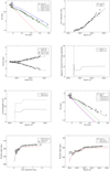 |
Fig. 10. Model-fitting results of the kinematics for knot C31. Bottom panels: the modeled relations between its observed position angle vs. core separation (left) and vs. time (right) are shown. The black lines denote the fitting model and the red lines indicate the precessing nozzle model. The black line and the red line coincide only at their initial parts near the core due to the trajectory curvatures in the outer jet regions. We note that several data points within core separation rn < 0.3 mas are located close to the precessing common parabolic trajectory. |
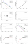 |
Fig. 11. Model-fitting results of the kinematics for knot C32. Bottom panels: the modeled relations between its observed position angle vs. core separation (left) and vs. time (right) are shown. The black lines denote the fitting model and the red lines indicate the precessing nozzle model. The black line and the red line coincide only at their initial parts near the core due to the trajectory curvatures in the outer jet regions. We note that several data points within core separation rn < 0.3 mas are located close to the modeled precessing common parabolic trajectory. |
Modeled ejection epoch t0 = 2010.94, precession phase ω = 2.58 rad. Its inner trajectory within core separation 0.30 mas (corresponding axial distance Z = 15 mas = 95.3 pc) is observed to closely follow the precessing common parabolic trajectory (ψ = 1.15 rad). There are a great number of data points (20 in total) located close to the precessing common trajectory, and thus its inner kinematics can be nicely explained in terms of the precessing nozzle model. For explaining its outer trajectory (rn > 0.30 mas) changes in parameter ψ have to be introduced to describe the trajectory curvatures: for Z = 15 − 20 mas ψ(rad)=1.15 − 0.22(Z − 15)/(20 − 15); for Z > 20 mas ψ = 0.93 rad. In order to explain its core separation versus time, an acceleration of its motion is required: for Z ≤ 10 mas Γ = 13; for Z = 10 − 15 mas Γ = 13 + 3(Z − 10)/(15 − 10); for Z > 15 mas Γ = 16.
In the bottom panels of Fig. 10, the modeled relations of its position angle versus core separation and versus time are shown. Within a core separation rn < 0.3 mas, there are a great number of data points (20 in total) located close to the precessing common trajectory, indicating that the precessing common parabolic trajectory has been firmly observed. These panels also reveal the large and rapid changes in its position angle near the core, demonstrating the process of transition of its position angle from ∼−200° to ∼−130°. The unusual ejection position angle of knot C31 at PA = ∼−200° is almost perpendicular to the usually observed jet direction (∼−130°). This behavior has been explained as being due to the change in its jet direction sweeping across the line of sight (Lu et al. 2013). The modeling studies here demonstrate an alternative interpretation. The kinematic properties of knot C31 can be naturally explained in our double precessing nozzle scenario with common parabolic trajectory shapes. In particular, the precession period of 25 yr is verified from the model-fitting of the kinematics of knot C31 combined with other knots of the group-2.
The modeled apparent velocity is consistent with the VLBI measured average apparent velocity 7.23 ± 0.40 c given by Jorstad et al. (2017).
7.2.6. Knot C32
The model-fitting results are shown in Fig. 11.
Modeled ejection epoch t0 = 2010.47, precession phase ω = 2.70 rad. Its inner trajectory within core separation rn = 0.31 mas (corresponding axial distance Z = 15 mas = 95.3 pc) can be modeled to follow the precessing common parabolic trajectory (ψ = 1.15 rad). There are several data points located close to the parabolic trajectory3. Thus, its inner kinematics can be understood in terms of the precessing nozzle model. Because the common trajectory has a parabolic pattern near the core, its modeled position angle rapidly changes with core separation. In order to explain its outer trajectory (rn > 0.31 mas) changes in the parameter ψ are introduced to describe the trajectory curvatures: for Z = 15 − 20 mas ψ(rad)=1.15 − 0.22(Z − 15)/(20 − 15); for Z > 20 mas ψ = 0.93 rad. To explain its core separation versus time, an acceleration of its motion is required: for Z ≤ 10 mas Γ = 11; for Z = 10 − 15 Γ = 11 + 2(Z − 10)/(15 − 10); for Z > 15 Γ = 13.
The modeled apparent velocity is consistent with the VLBI measured average apparent velocity 5.35 ± 0.53 c given by Jorstad et al. (2017).
In the bottom panels of Fig. 11, the modeled relations of its position angle versus core separation and versus time are shown, which reveal the large and rapid changes in its position angle near the core. The precessing common parabolic trajectory has been firmly observed and the 25 yr precession period is verified.
We emphasize that the kinematic features of knots C27, C28, C29, C30, C31, and C32, combined with those of knots C5a, C6, C7, and C17–C20, can be consistently interpreted in terms of the precessing nozzle model with a precession period of 25 yr. This result seems very important, verifying the double-jet structure and the common parabolic trajectory pattern near the core in blazar 3C279.
7.3. Brief summary of jet-B
We have presented the model-fitting results of the kinematics for the 13 superluminal components of jet-B. The kinematic features of most of the knots are consistently fitted in terms of the precessing nozzle model. The model-fitting of the kinematics for knots C5a–C20 observed during the period 1991–2004 and model-fitting of the kinematics for knots C27–C32 observed during the period 2008–2015 have been unified into a precessing jet nozzle scenario. This may be regarded as evidence for the existence of a second jet (jet-B). The double precessing nozzle scenario with a 25 yr precession period (±2.5 yr) proposed in this paper are validated. The parabolic pattern assumed for the precessing common trajectory is also verified, having been observed in several knots.
In Table 6 are summarized the core separations within which the precessing common trajectories were observed. Nine (marked with symbol “+”) out of the 13 knots (occupying ∼70%) are observed to follow the precessing common trajectory in their innermost jet regions (core separations range from 0.044 mas to 0.31 mas, or radial distance Z from 0.64 pc to 95 pc). For the other four knots (marked with symbol “–”) their innermost trajectory could also follow the precessing common trajectory, but this is not determined due to the lack of observation data at their separations close to the core.
We note that the detailed kinematics, especially the detailed tracks at core separations 0.1–0.5 mas, measured by 43 GHz VLBI observations (Jorstad et al. 2017) for knots C27–C32 have been proved to be very useful to determine the properties of the second jet. The detailed tracks and kinematics measured for knots C30–C32 are particularly important. Combined with the model-fitting of the kinematics for knots C5a–C20, they not only indicate the 25 yr precession period for the second jet (jet-B) and validate the parabolic pattern for the precessing common trajectory, verifying our double precessing jet scenario for 3C279, they also demonstrate the transition from the precessing parabolic tracks (in the innermost regions) to trajectory curvatures (in the outer regions). The consistency of the kinematics of the six knots (C27–C32, ejected in two years) during a time interval of ∼7 yr (2008–2015) may strongly indicate that they are all ejected from jet-B independent of jet-A. The remarkable change in the jet direction in late 2010 when knot C31 was ejected at position angle ∼−200° can now be explained as its ejection from jet-B with a position angle very different from those usually ejected from jet-A. Its position angle rapidly changed during the period 2010–2012 (or in the separation range 0.1–0.3 mas) as shown in Fig. 10 (bottom panels). This can be regarded as an alternative explanation instead of the suggestion of a single jet (jet-A) sweeping across the line of sight (Agudo et al. 2011, 2007; Lu et al. 2013).
In Figs. B.5–B.7 and Figs. 9–11, the model-fittings of the position angle versus separation and versus time (last two panels) for knots C27–C32 are shown. It can be seen that for knot C30–C32 these model fits within separation rn < 0.2 − 0.3 mas, which indicates that the assumed parabolic trajectory pattern is appropriate and confirms their highly curved trajectories. For knots C27, C28, and C29 (Figs. B.5–B.7) there are no data to confirm their highly curved trajectories. However, given that all six knots are ejected within 1–2 years, the kinematic behavior should be similar to that of knots C30–C32. This can be seen in the similar behaviors shown in their similar rn-PA relations.
8. Conclusion
We have analyzed and model-fitted the parsec-scale kinematics of the 31 superluminal components observed in blazar 3C279 during a 34 yr period (1981–2015). Regular motion along the precessing common trajectory in the innermost regions and the trajectory curvatures at different separations are both taken into account. We find that the kinematic properties of most of the knots can be well interpreted in terms of the double precessing jet scenario. However, for most of the knots their precession common trajectories have been observed in the core separations rn < 0.1 − 0.2 mas, thus higher resolution VLBI observations are needed to closely monitor their kinematics near the core.
Several significant results can be summarized: (1) 3C279 may have a double-jet structure (designated jet-A and jet-B), having different orientations in space. They both eject superluminal components and both jets precess with the same precession period of 25 yr and along the same direction; (2) the 31 superluminal components can be divided into two groups, which are ejected from jet-A and jet-B. The modeled position angle versus ejection epoch (for separation 0.15 mas) is shown in Fig. 124, where the modeled relations for jet-A and jet-B are superimposed and clearly demonstrate the ejection of superluminal components from both jets at different position angles at the same times, sometimes resulting in “illusions” of large swings in jet direction; (3) for both jet-A and jet-B, the innermost kinematics of the knots can be model-fitted in terms of the precessing nozzle model with the model parameters given in Tables 1 and 4, respectively. Their outer kinematics can be interpreted by introducing trajectory curvatures described by changes in the parameter ψ, as noted in Sects. 6 and 7 for the individual knots. The model-fitting results include trajectory, core separation, and apparent velocity. Viewing angle and Lorentz/Doppler factor are derived. Acceleration or deceleration of their motion have been taken into account. By utilizing the derived Doppler factor versus time for each of the knots, combined with multifrequency radio light curves, the intrinsic evolution of the knots and their physical parameters can be investigated; (4) a double-jet structure implies a binary black hole system existing at the center of 3C279. The primary and the secondary supermassive black hole both produce a relativistic jet, ejecting superluminal components frequently. Since the two jets have the same precession period of 25 yr, the precession of the jets may originate from the modulation of the jet directions caused by the orbital motion of the primary and secondary holes (Roos et al. 1993). In this case the mass ratio (m/M) of the binary approximately equals the ratio of the orbital velocities of the binary or the ratio of the (projected) jet-cone widths. This is on the order of ∼0.5 (Fig. 12; right panels); (5) as shown in Figs. 2 and 12 (right panels), jet-B has a much wider cone aperture than that of jet-A. Thus, jet-B may be attributed to the secondary supermassive hole and jet-A to the primary supermassive hole. Because the secondary has a smaller mass, its orbital velocity should be larger than that of the primary, implying that the modulation of the direction of the secondary jet by its orbital motion should be larger. Moreover, hydrodynamic/magnetohydrodynamic (HD/MHD) simulations of cavity-accretion in binary supermassive black hole systems have shown that gas-streams preferentially accrete onto the secondary (Tanaka 2013; Artymovicz & Lubow 1996; Cuadra et al. 2009; Shi et al. 2012), thus the secondary jet would be more active than the primary jet. The optical and radio observations by Cheung (2002) have confirmed this deduction; (6) Cheung (2002) reported the detection of the optical synchrotron emission from the kpc-scale radio jet of 3C279. This radio jet extends out to ∼5 arcseconds (15 GHz, VLA (Very Large Array)) at a position angle of ∼–155°, indicating its lifetime of ∼106 yr at least. Interestingly, this kpc-jet is just the extension of jet-B5, which we have been looking for since 2013 (Qian 2013). Now we recognize that the kpc-counterpart of jet-B has existed for at least ∼106 years and had already been observed in 1982 (de Pater & Perley 1983). In fact, jet-B itself had been observed as a milliarcsecond jet in 1970s at position angle ∼–150° (Pauliny-Toth et al. 1981; Cotton et al. 1979; Niell et al. 1975). We are now aware of the existence of jet-B: just owing to its activity during 2008–2015 ejecting superluminal components C25–C32 (Jorstad et al. 2017) and our model-fitting for the kinematics of the 13 knots (C5a–C7, C17–C20, and C27–C32), showing that they are all ejected from the precessing nozzle of jet-B. We further point out that on pc-scales all the superluminal knots move along parabolic trajectories with prominent curvatures with position angles in the range of ∼ − 120° to ∼ − 130° (at core separations > 1 mas), but the kpc-jet (at PA ∼ −155°) is extremely straight with its position angle connected to the pc-jet axis (∼ − 155°). This may imply that these superluminal knots are moving along helical trajectories of decreasing pitch angles on ∼0.1–1 kpc around the pc-jet axis, i.e., the superluminal knots are aligned (collimated) at kpc-scales. The orientation of the axis of the jet-B cone has been present in space for ∼106 yr with a long-term stability. Obviously, the axis of the jet-B cone and the axis of the kpc-jet may represent the spin axis of the secondary black hole. The radio maps obtained by Cheung (2002) do not show any trails of jet-A, indicating that its much weaker activity with respect to jet-B may be due to the much lower accretion rate onto the primary hole, as predicted by HD/MHD simulations of cavity-accretion in binary systems6; and (7) the unusual behavior of knot C31 (its ejection position angle being almost perpendicular to the position angle usually observed, Jorstad et al. 2017; Lu et al. 2013 can now be naturally explained (see upper left and bottom left panels of Fig. 10). Knots C27–C32 should have been ejected at position angles (∼−200°) in 2008–2010, as predicted by the precession model for jet-B with initial trajectories having a parabolic form near the core. Thus, the remarkable change in the jet direction observed in late 2010 when knot C31 appeared may not imply a single jet sweeping across the line of sight (Lu et al. 2013).
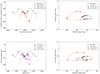 |
Fig. 12. Top two panels: modeled variations of the knot’s ejection position angle with its ejection time and the modeled relation between the ejection position angle vs. its ejection viewing angle. Bottom two panels: observed variations of the knot’s ejection position angle with ejection time and the observed distribution of the knot’s ejection position angle vs. its ejection viewing angle. The curves and the quantities are calculated by using the precession jet nozzle model for core separation rn = 0.15 mas. The viewing angle ranges from 1.22° to 1.48° (jet-A) and from 1.17° to 1.76° (jet-B). |
The chief results of this work can briefly be summarized as follows: (1) blazar 3C279 may have a double-jet structure produced by a supermassive black hole binary; (2) regular jet precession may exist in 3C279 and both jets precess with the same period of 25 yr. For a large number of the superluminal knots (∼70%) their ejection epochs have been model-fitted to confirm this precession period within an uncertainty of ±2.5 yr; (3) the superluminal knots may move along precessing common trajectories having parabolic patterns in their innermost jet regions; and (4) for a large percentage of the superluminal knots (∼70%) their innermost trajectory has been observed to follow the precessing common parabolic trajectory.
The double precessing nozzle model proposed as the interpretation of the kinematic features on parsec scales in blazar 3C279 may be significant and useful for understanding the kinematics of other blazars. For example, searching double-jet structures in blazars (e.g., 3C345, 3C454.3, 3C273, and OJ287) may be useful. Additional VLBI monitoring observations at higher resolutions may be helpful to reveal the real mechanisms of ejection of superluminal components, especially the processes in the central hole–disk system around binary Kerr black holes. Magnetohydrodynamic theories on the formation, collimation, and acceleration of relativistic jets and jet-accretion-black hole interaction in binary systems are very much required. If some blazars are binary black hole candidates, then they will become the objects used for the detection of gravitational waves (GW) (Einstein 1916, 1918) by using future GW space observatories.
Knots K2 and K3 were designated as knots C27–C29 in Jorstad et al. (2017).
Roland et al. (2013) attempted to explain the different trajectories followed by the knot C5 and knot C10 in terms of a binary black hole system.
The deviation of these data points from the precessing common trajectory might be due to uncertainties in VLBI image-modeling; its entire trajectory was observed to be very similar to that of knot C30 and C31 and the three knots were ejected in a very narrow phase range 2.58 rad (knot C31) to 2.70 rad (knot C32). Thus, the innermost trajectory of knot C32 (rn < 0.3 mas) should be regarded to be well fitted by the precessing common trajectory.
In the case of highly curved trajectories, we can only study the position angle swing at a common separation (e.g., Qian et al. 2009).
It is quite surprising and beyond our expectation that the axis of the southern jet (jet-B) was derived from our model-fitting in terms of a precessing double-jet scenario to be at PA∼–157° (Fig. 2), almost exactly equal to that of the kpc-jet measured by VLA Cheung (2002) and de Pater & Perley (1983). This implies that our precessing double-jet scenario and the model-fitting assumptions (and procedure) are valid and effective.
Component A on the 6 cm map (Fig. 1 in de Pater & Perley 1983) might be a remnant extension of jet-A.
Acknowledgments
We would like to thank the anonymous referee for introducing the earlier VLA observations of 3C279 by Cheung (2002), which posteriorly verified the existence of jet-B derived from the model-fitting of the kinematics of the superluminal components in terms of our precessing double-jet nozzle scenario. Qian wishes to express thanks to Yi-Min Teng (National Astronomical Observatories of Chinese Academy of Sciences) for his long-lasting help with the preparation of our papers. We thank Dr. S.G. Jorstad (Boston University, USA) for providing the 43 GHz VLBI data on knots C24–C32, which were essential for this work. This study makes use of 43 GHz VLBA data from the VLBA-BU Blazar Monitoring Program, funded by NASA through the Fermi Guest investigator Program. The VLBA is an instrument of the Long Baseline Observatory. The Long Baseline Observatory is a facility of the National Science Foundation operated by Associated Universities, Inc.
References
- Abdo, A. A., Ackermann, M., Agudo, I., et al. 2010, ApJ, 716, 30 [NASA ADS] [CrossRef] [Google Scholar]
- Abraham, Z., & Carrara, E. A. 1998, ApJ, 496, 172 [NASA ADS] [CrossRef] [Google Scholar]
- Ackermann, M., Anantua, R., Asano, K., et al. 2016, ApJ, 824, L20 [NASA ADS] [CrossRef] [Google Scholar]
- Agarwal, A., Mohan, P., Gupta, A. C., et al. 2017, MNRAS, 469, 813 [NASA ADS] [CrossRef] [Google Scholar]
- Agudo, I., Bach, U., Krichbaum, T. P., et al. 2007, A&A, 476, L17 [NASA ADS] [CrossRef] [EDP Sciences] [Google Scholar]
- Agudo, I., Jorstad, S. G., Marscher, A. P., et al. 2011, ApJ, 726, L13 [NASA ADS] [CrossRef] [Google Scholar]
- Albert, J., Aliu, E., Anderhub, H., et al. 2008, Science, 320, 1752 [NASA ADS] [CrossRef] [PubMed] [Google Scholar]
- Aleksić, J., Antonelli, L. A., Antoranz, P., et al. 2011, A&A, 530, A4 [NASA ADS] [CrossRef] [EDP Sciences] [Google Scholar]
- Aleksić, S., Ansoldi, S., Antonelli, L. A., et al. 2014, A&A, 567, A41 [NASA ADS] [CrossRef] [EDP Sciences] [Google Scholar]
- Arbeiter, C., Pohl, M., Schlickeiser, R., et al. 2005, ApJ, 627, 62 [NASA ADS] [CrossRef] [Google Scholar]
- Artymovicz, P., & Lubow, S. H. 1996, ApJ, 467, L77 [NASA ADS] [CrossRef] [Google Scholar]
- Asada, K., & Nakamura, M. 2012, ApJL, 745, L28 [CrossRef] [Google Scholar]
- Bach, U., Krichbaum, T. P., Ros, E., et al. 2005, A&A, 433, 815 [NASA ADS] [CrossRef] [EDP Sciences] [Google Scholar]
- Begelman, M. C., Blandford, R. D., & Rees, M. J. 1980, Nature, 287, 307 [NASA ADS] [CrossRef] [Google Scholar]
- Blandford, R. D., & Payne, D. G. 1982, MNRAS, 199, 883 [NASA ADS] [CrossRef] [Google Scholar]
- Blandford, R. D., & Znajek, R. L. 1977, MNRAS, 179, 433 [NASA ADS] [CrossRef] [Google Scholar]
- Carrara, E. A., Abraham, Z., Unwin, S. C., & Zensus, J. A. 1993, A&A, 279, 83 [NASA ADS] [Google Scholar]
- Chatterjee, R., Jorstad, S. G., Marscher, A. P., et al. 2008, ApJ, 689, 79 [NASA ADS] [CrossRef] [Google Scholar]
- Chatterjee, R., Bailyn, C. D., Bonning, E. W., et al. 2012, ApJ, 749, 191 [NASA ADS] [CrossRef] [Google Scholar]
- Cheung, C. C. 2002, ApJ, 581, L15 [NASA ADS] [CrossRef] [Google Scholar]
- Cohen, M. H., Cannon, W., Purcell, G. H., et al. 1971, ApJ, 170, 207 [NASA ADS] [CrossRef] [Google Scholar]
- Cohen, D. P., Romani, R. W., Filippenko, A. V., et al. 2014, ApJ, 797, 137 [NASA ADS] [CrossRef] [Google Scholar]
- Collmar, W., Böttcher, M., Krichbaum, T. P., et al. 2010, A&A, 522, A66 [NASA ADS] [CrossRef] [EDP Sciences] [Google Scholar]
- Cotton, W. D., Counselman, III, C. C., Geller, R. B., et al. 1979, ApJ, 229, L115 [NASA ADS] [CrossRef] [Google Scholar]
- Cuadra, J., Amitage, P. J., Alexander, R. D., et al. 2009, MNRAS, 393, 1423 [NASA ADS] [CrossRef] [Google Scholar]
- de Pater, I., & Perley, R. A. 1983, ApJ, 273, 64 [NASA ADS] [CrossRef] [Google Scholar]
- Dermer, C. D., Finke, J. D., Krug, H., & Böttcher, M. 2009, ApJ, 692, 32 [NASA ADS] [CrossRef] [Google Scholar]
- Einstein, A. 1916, Sitzungberichte der Königlich Preusssichen Akademie der Wissenshafte (Berlin: SPAW), 688 [Google Scholar]
- Einstein, A. 1918, Sitzungberichte der Königlich Preusssichen Akademie der Wissenshafte (Berlin: SPAW), 154 [Google Scholar]
- Gu, M., Cao, X., & Jiang, D. R. 2001, MNRAS, 327, 111 [Google Scholar]
- Hartman, R. C., Bertsch, D. L., Fichtel, C. E., et al. 1992, ApJ, 385, L1 [NASA ADS] [CrossRef] [Google Scholar]
- Hayashida, M., Madejski, G. M., Nalewajko, K., et al. 2012, ApJ, 754, 114 [NASA ADS] [CrossRef] [Google Scholar]
- Hayashida, M., Nalewajko, K., Madejski, G. M., et al. 2015, ApJ, 807, 79 [Google Scholar]
- Hogg, D. W. 1999, ArXiv e-prints [arXiv:astro-ph/9905116] [Google Scholar]
- Homan, D. C., Lister, M. L., Kellermann, K. I., et al. 2003, ApJ, 589, L9 [NASA ADS] [CrossRef] [Google Scholar]
- Hovatta, T., Valtaoja, E., Tornikoski, M., & Lähteenmäki, A. 2009, A&A, 494, 527 [NASA ADS] [CrossRef] [EDP Sciences] [Google Scholar]
- Isler, J. C., Urry, C. M., Coppi, P., et al. 2017, ApJ, 844, 107 [NASA ADS] [CrossRef] [Google Scholar]
- Jorstad, S. G., & Marscher, A. P. 2005, Mem. S.A.It., 76, 106 [NASA ADS] [Google Scholar]
- Jorstad, S. G., & Marscher, A. P. 2016, Galaxies, 4, 471 [NASA ADS] [CrossRef] [Google Scholar]
- Jorstad, S. G., Marscher, A. P., Lister, M. L., et al. 2004, AJ, 127, 3115 [NASA ADS] [CrossRef] [EDP Sciences] [Google Scholar]
- Jorstad, S. G., Marscher, A. P., Stevens, J. A., et al. 2007, AJ, 134, 799 [NASA ADS] [CrossRef] [Google Scholar]
- Jorstad, S. G., Marscher, A. P., Agudo, I., & Harrison, B. 2011, Fermi Symp. Proc., eConf C110509 [Google Scholar]
- Jorstad, S. G., Marscher, A. P., Morozova, D. A., et al. 2017, ApJ, 846, 98 [NASA ADS] [CrossRef] [Google Scholar]
- Kang, S., Lee, S.-S., & Byun, D.-Y. 2015, J. Korean Astron. Soc., 48, 257 [NASA ADS] [CrossRef] [Google Scholar]
- Kniffen, D. A., Bertsch, D. L., Fichtel, C. E., et al. 1993, ApJ, 411, 133 [NASA ADS] [CrossRef] [Google Scholar]
- Larionov, V. M., Jorstad, S. G., Marscher, A. P., et al. 2008, A&A, 492, 389 [NASA ADS] [CrossRef] [EDP Sciences] [Google Scholar]
- Lewis, T. R., Finke, J. D., & Becker, P. A. 2018, ApJ, 853, 6 [NASA ADS] [CrossRef] [Google Scholar]
- Li, Z. Y., Chiueh, T., & Begelman, M. C. 1992, ApJ, 394, 459 [NASA ADS] [CrossRef] [Google Scholar]
- Lister, M. L., & Marscher, A. P. 1997, ApJ, 476, 572 [NASA ADS] [CrossRef] [Google Scholar]
- Lister, M. L., Aller, M. F., Aller, H. D., et al. 2013, ApJ, 146, 120 [Google Scholar]
- Lobanov, A. P., & Roland, J. 2005, A&A, 431, 831 [NASA ADS] [CrossRef] [EDP Sciences] [Google Scholar]
- Lu, R. S., Fish, V. L., Akiyama, K., et al. 2013, ApJ, 772, 13 [NASA ADS] [CrossRef] [Google Scholar]
- MacDonald, N. R., Marscher, A. P., Jorstad, S. G., & Joshi, M. 2014, AAS, 224, 410.02 [NASA ADS] [Google Scholar]
- Mannheim, K. 1993, A&A, 269, 27 [Google Scholar]
- Marscher, A. P. 2008, in in Extragalactic Jets: Theory and Observation from Radio to Gamma-Ray, eds. T. A. Rector, & D. S. De Young, ASP Conf. Ser., 386, 437 [NASA ADS] [Google Scholar]
- Marscher, A. P. 2009, in Approaching Micro-Arcsecond Resolution with VSOP-2: Astrophysics and Technologies, eds. Y. Hagiwara, E. Fomalont, M. Tsuboi, & M. Yasuhiro, ASP Conf. Ser., 402, 194 [NASA ADS] [Google Scholar]
- Marscher, A. P., & Jorstad, S. G. 2011, ApJ, 726, 29 [NASA ADS] [CrossRef] [Google Scholar]
- Marscher, A. P., Jorstad, S. G., Larionov, V. M., et al. 2010, ApJ, 710, L126 [NASA ADS] [CrossRef] [Google Scholar]
- Marscher, A. P., Jorstad, S. G., Agudo, I., et al. 2012, Fermi & Jansky Proc., eConf, C1111101 [Google Scholar]
- Marscher, A. P., Jorstad, S. G., & Williamson, K. E. 2017, Galaxies, 5, 63 [NASA ADS] [CrossRef] [Google Scholar]
- Maraschi, L., Ghisellini, G., & Celotti, A. 1992, ApJ, 397, L5 [NASA ADS] [CrossRef] [Google Scholar]
- Meier, D. L., & Nakamura, M. 2006, in Blazar Variability Workshop II: Entering the GLAST Era, eds. H. R. Miller, K. Marshall, J. R. Webb, & M. F. Aller, ASP Conf. Ser., 350, 195 [NASA ADS] [Google Scholar]
- Meier, D. L., Koide, S., & Uchida, Y. 2001, Science, 291, 84 [NASA ADS] [CrossRef] [PubMed] [Google Scholar]
- Nakamura, M., & Asada, K. 2013, ApJ, 775, 118 [NASA ADS] [CrossRef] [Google Scholar]
- Niell, A. E., Kellermann, K. I., Clark, B. G., et al. 1975, ApJ, 197, L109 [NASA ADS] [CrossRef] [Google Scholar]
- Nilsson, K., Pursimo, T., Villforth, C., et al. 2009, A&A, 505, 601 [NASA ADS] [CrossRef] [EDP Sciences] [Google Scholar]
- Paliya, V. S. 2015, ApJ, 808, L48 [NASA ADS] [CrossRef] [Google Scholar]
- Pauliny-Toth, I. I. K., Preuss, E., Witzel, A., et al. 1981, AJ, 86, 371 [NASA ADS] [CrossRef] [Google Scholar]
- Pen, U.-L. 1999, ApJS, 120, 49 [NASA ADS] [CrossRef] [Google Scholar]
- Petropoulou, M., Giannios, D., & Sironi, L. 2016, MNRAS, 462, 3325 [NASA ADS] [CrossRef] [Google Scholar]
- Petropoulou, M., Nalewajko, K., Hayashida, M., & Mastichiadis, A. 2017, MNRAS, 467, L16 [NASA ADS] [CrossRef] [Google Scholar]
- Polko, P., Meier, D. L., & Markoff, S. 2010, ApJ, 723, 1343 [NASA ADS] [CrossRef] [Google Scholar]
- Polko, P., Meier, D. L., & Markoff, S. 2013, MNRAS, 428, 587 [NASA ADS] [CrossRef] [Google Scholar]
- Polko, P., Meier, D. L., & Markoff, S. 2014, MNRAS, 438, 959 [NASA ADS] [CrossRef] [Google Scholar]
- Qian, S. J. 2011, Res. Astron. Astrophys., 11, 43 [NASA ADS] [CrossRef] [Google Scholar]
- Qian, S. J. 2012, Res. Astron. Astrophys., 12, 46 [NASA ADS] [CrossRef] [Google Scholar]
- Qian, S. J. 2013, Res. Astron. Astrophys., 13, 783 [NASA ADS] [CrossRef] [Google Scholar]
- Qian, S. J. 2015, Res. Astron. Astrophys., 15, 687 [NASA ADS] [CrossRef] [Google Scholar]
- Qian, S. J. 2016, Res. Astron. Astrophys., 16, 20 [NASA ADS] [CrossRef] [Google Scholar]
- Qian, S. J., Witzel, A., Krichbaum, T. P., et al. 1991. Acta Astron. Sin., 32, 369 (english translation in Chin. Astron. Astrophys., 1992, 16, 137) [Google Scholar]
- Qian, S. J., Krichbaum, T. P., Zensus, J. A., et al. 1996, A&A, 308, 395 [NASA ADS] [Google Scholar]
- Qian, S. J., Witzel, A., Zensus, J. A., et al. 2009, Res. Astron. Astrophys., 9, 137 [NASA ADS] [CrossRef] [Google Scholar]
- Qian, S. J., Krichbaum, T. P., Witzel, A., et al. 2010, Res. Astron. Astrophys., 10, 47 [NASA ADS] [CrossRef] [Google Scholar]
- Qian, S. J., Britzen, S., Witzel, A., et al. 2014, Res. Astron. Astrophys., 14, 249 [NASA ADS] [CrossRef] [Google Scholar]
- Qian, S. J., Britzen, S., Witzel, A., et al. 2017, A&A, 604, A90 [NASA ADS] [CrossRef] [EDP Sciences] [Google Scholar]
- Qian, S. J., Britzen, S., Witzel, A., et al. 2018, A&A, 615, A123 [NASA ADS] [CrossRef] [EDP Sciences] [Google Scholar]
- Rani, B., Krichbaum, T. P., Lee, S.-S., et al. 2017, MNRAS, 464, 418 [NASA ADS] [CrossRef] [Google Scholar]
- Raiteri, C. M., Villata, M., Bruschini, L., et al. 2010, A&A, 524, A43 [NASA ADS] [CrossRef] [EDP Sciences] [Google Scholar]
- Roland, J., Britzen, S., Caproni, A., et al. 2013, A&A, 557, A85 [Google Scholar]
- Roos, N., Kaastra, J. S., & Hummel, C. A. 1993, ApJ, 409, 130 [NASA ADS] [CrossRef] [Google Scholar]
- Savolainen, T., Wiik, K., Valtaoja, E., & Tornikoski, M. 2006, A&A, 446, 71 [NASA ADS] [CrossRef] [EDP Sciences] [Google Scholar]
- Schinzel, F. K., Lobanov, A. P., Jorstad, S. G., et al. 2010, in Fermi meets Jansky - AGN in Radio and Gamma-Rays, eds. T.Savolainen, E.Ros, R. W.Porcas, & J. A.Zensus, 175 [Google Scholar]
- Shi, J.-M., Krolik, J. H., Lubow, S. H., et al. 2012, ApJ, 749, 118 [NASA ADS] [CrossRef] [Google Scholar]
- Sikora, M., Begelman, M. C., & Rees, M. J. 1994, ApJ, 421, 153 [NASA ADS] [CrossRef] [Google Scholar]
- Spergel, D. N., Verde, L., Peiris, H. V., et al. 2003, ApJS, 148, 175 [NASA ADS] [CrossRef] [Google Scholar]
- Steffen, W., Zensus, J. A., Krichbaum, T. P., Witzel, A., & Qian, S. J. 1996, A&A, 302, 335 [NASA ADS] [Google Scholar]
- Stirling, A. M., Cawthorne, T. V., Stevens, J. A., et al. 2003, MNRAS, 341, 405 [NASA ADS] [CrossRef] [Google Scholar]
- Tanaka, T. L. 2013, MNRAS, 434, 2275 [NASA ADS] [CrossRef] [Google Scholar]
- Unwin, S. C., Cohen, M. H., Birreta, J. A., et al. 1989, ApJ, 340, 117 [NASA ADS] [CrossRef] [Google Scholar]
- Vercellone, S., D’ammando, F., & Vittorini, V., et al. 2010, ApJ, 712, 405 [NASA ADS] [CrossRef] [Google Scholar]
- Vittorini, V., Tavani, M., & Cavaliere, A. 2017, ApJ, 843, L23 [NASA ADS] [CrossRef] [Google Scholar]
- Vlahakis, N., & Koenigl, A. 2004, ApJ, 605, 656 [NASA ADS] [CrossRef] [Google Scholar]
- Wehrle, A. E., Piner, B. G., Unwin, S. C., et al. 2001, ApJS, 133, 297 [NASA ADS] [CrossRef] [Google Scholar]
- Whitney, A. R., Shapiro, I. I., Rogers, A. E. E., et al. 1971, Science, 173, 225 [NASA ADS] [CrossRef] [Google Scholar]
- Woo, J.-H., & Urry, C. M. 2002, ApJ, 579, 530 [NASA ADS] [CrossRef] [Google Scholar]
Appendix A: Figures for northern jet (jet-A)
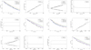 |
Fig. A.1. Model-fitting results of the kinematic features for knot C9 (first 6 panels, from top left to bottom right) and for knot C10 (last six panels) including trajectory, coordinates, core separation, apparent velocity, viewing angle, Lorentz factor, and Doppler factor. In the 1st and 7th panels, the green and blue lines represent the fitting model trajectories calculated for the precession phases ω ± 0.63 rad. In the 6th and 12th panels, the green and blues represent the precessing common parabolic trajectories calculated for the precession phases ω ± 0.63 rad. For knot C10 one innermost data point is within the position angle range defined by the two lines, indicating that its innermost trajectory has been observed to follow the precessing common parabolic trajectory. |
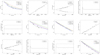 |
Fig. A.2. Model-fitting results of the kinematic features for knot C11 (first 6 panels, from top left to bottom right) and for knot C12 (last six panels) including trajectory, core separation, coordinates, apparent velocity, viewing angle, Lorentz factor, and Doppler factor. In the 1st and 7th panels, left panels, the green and blue lines represent the fitting model trajectories calculated for the precession phases ω ± 0.63 rad. In the 6th and 12th panels, the green and blue lines represent the precessing common parabolic trajectories calculated for the precession phases ω ± 0.63 rad. For knot C12 a few data points are within the position angle range defined by the two lines, indicating that its innermost trajectory has been observed to follow the precessing common parabolic trajectory. |
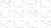 |
Fig. A.3. Model-fitting results of the kinematic features for knot C13 (first 6 panels, from top left to bottom right) and for knot C14 (last six panels) including trajectory, core separation, coordinates, apparent velocity, viewing angle, Lorentz factor, and Doppler factor. In the 1st and 7th panels, the green and blue lines represent the fitting model trajectories calculated for the precession phases ω ± 0.63 rad. In the 6th and 12th panels, the green and blue lines represent the precessing common parabolic trajectories calculated for the precession phases ω ± 0.63 rad. For both C13 and C14 a few data points are within the position angle range defined by the two lines, indicating that their innermost trajectories have been observed to follow the precessing common parabolic trajectory. |
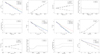 |
Fig. A.4. Model-fitting results of the kinematic features for knot C15 (first 6 panels, from top left to bottom right) and for knot C16 (last six panels) including trajectory, core separation, coordinates, apparent velocity, viewing angle, Lorentz factor, and Doppler factor. In the 1st and 7th panels, the green and blue lines represent the fitting model trajectories calculated for precession phases ω ± 0.63 rad. In the 6th and 12th panels, the green and blue lines represent the precessing common parabolic trajectories calculated for precession phases ω ± 0.63 rad. For both C15 and C16 a few data points are within the position angle range defined by the two lines, indicating that their innermost trajectories have been observed to follow the precessing common parabolic trajectory. |
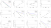 |
Fig. A.5. Model-fitting results of the kinematic features for knot C21 (first 6 panels, from top left to bottom right) and for knot C22 (last six panels) including trajectory, core separation, coordinates, apparent velocity, viewing angle, Lorentz factor, and Doppler factor. In the 1st and 7th panels, the green and blue lines represent the fitting model trajectories calculated for the precession phases ω ± 0.63 rad. In the 6th and 12th panels, the green and blue lines represent the precessing common parabolic trajectories calculated for the precession phases ω ± 0.63 rad. |
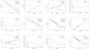 |
Fig. A.6. Model-fitting results of the kinematic features for knot C23 (first 6 panels, from top left to bottom right) and for knot C24 (last six panels) including trajectory, core separation, coordinates, apparent velocity, viewing angle, Lorentz factor, and Doppler factor. In the 1st and 7th panels, the green and blue lines represent the fitting model trajectories calculated for precession phases ω ± 0.63 rad. In the 6th and 12th panels, the green and blue lines represent the precessing common parabolic trajectories calculated for precession phases ω ± 0.63 rad. For both C23 and C24 a number of data points are within the position angle range defined by the two lines, indicating that their innermost trajectories have been observed to follow the precessing common parabolic trajectory. |
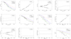 |
Fig. A.7. Model-fitting results of the kinematic features for knot C25 (first 6 panels, from top left to bottom right) and for knot C26 (last six panels) including trajectory, core separation, coordinates, apparent velocity, viewing angle, Lorentz factor, and Doppler factor. In the 1st and 7th panels, the green and blue lines represent the fitting model trajectories calculated for precession phases ω ± 0.63 rad. In the 6th and 12th panels, the green and blue lines represent the precessing common parabolic trajectories calculated for precession phases ω ± 0.63 rad. |
Appendix B: Figures for southern jet (jet-B)
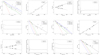 |
Fig. B.1. Model-fitting results of the kinematic features for knot C5a (first 6 panels, from top left to bottom right) and for knot C6 (last six panels) including trajectory, core separation, coordinates, apparent velocity, viewing angle, Lorentz factor, and Doppler factor. In the 1st and 7th panels, the green and blue lines represent the fitting model trajectories calculated for precession phases ω ± 0.63 rad. In the 6th and 12th panels, the green and blue lines represent the precessing common parabolic trajectories calculated for precession phases ω ± 0.63 rad. |
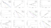 |
Fig. B.2. Model-fitting results of the kinematic features for knot C7 (first 6 panels, from top left to bottom right) and for C17 (last six panels) including trajectory, core separation, coordinates, apparent velocity, viewing angle, Lorentz factor, and Doppler factor. In the 1st and 7th panels, the green and blue lines represent the fitting model trajectories calculated for precession phases ω ± 0.63 rad. In the 6th and 12th panels, the green and blue lines represent the precessing common parabolic trajectories calculated for precession phases ω ± 0.63 rad. |
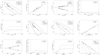 |
Fig. B.3. Model-fitting results of the kinematic features for knot C18 (first 6 panels, from top left to bottom right) and for knot C19 (last six panels) including trajectory, core separation, coordinates, apparent velocity, viewing angle, Lorentz factor, and Doppler factor. In the 1st and 7th panels, the green and blue lines represent the fitting model trajectories calculated for the precession phases ω ± 0.63 rad. In the 6th and 12th panels, the green and blue lines represent the precessing common parabolic trajectories calculated for precession phases ω ± 0.63 rad. |
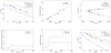 |
Fig. B.4. Model-fitting results of the kinematic features for knot C20 including trajectory, core separation, coordinates, apparent velocity, viewing angle, Lorentz factor, and Doppler factor. Upper left panel: the green and blue lines represent the fitting model trajectories calculated for precession phases ω ± 0.63 rad. Bottom right panel: the green and blue lines represent the precessing common parabolic trajectories calculated for precession phases ω ± 0.63 rad. |
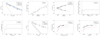 |
Fig. B.5. Model-fitting results of the kinematic features for knot C27 including trajectory, core separation, coordinates, apparent velocity, viewing angle, Lorentz factor, and Doppler factor. In the first panel, the green and blue lines represent the fitting model trajectories calculated for precession phases ω ± 0.63 rad. In the 6th panel, the green and blue lines represent the precessing common parabolic trajectories calculated for precession phases ω ± 0.63 rad. In the last two panels the relations of the knot’s position angle vs. core separation and vs. time are shown. |
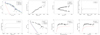 |
Fig. B.6. Model-fitting results of the kinematic features for knot C28 including trajectory, core separation, coordinates, apparent velocity, viewing angle, Lorentz factor, and Doppler factor. In the first panel, the green and blue lines represent the fitting model trajectories calculated for precession phases ω ± 0.63 rad. In the 6th panel, the green and blue lines represent the precessing common parabolic trajectories calculated for precession phases ω ± 0.63 rad. In the last two panels, the relations of the knot’s position angle vs. core separation and vs. time are shown. |
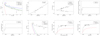 |
Fig. B.7. Model-fitting results of the kinematic features for knot C29 including trajectory, core separation, coordinates, apparent velocity, viewing angle, Lorentz factor, and Doppler factor. In the first panel, the green and blue lines represent the fitting model trajectories calculated for precession phases ω ± 0.63 rad. In the 6th panel, the green and blue lines represent the precessing common parabolic trajectories calculated for precession phases ω ± 0.63 rad. In the last two panels the relations of the knot’s position angle vs. core separation and vs. time are shown. |
All Tables
Jet-A: core separations (rn) and corresponding axial distances (Z) within which the knots move along the precessing common trajectory.
Model parameters of the precessing nozzle model with a period of 25 yr for jet-B.
Core separations rn within which the knots of jet-B follow the precessing common trajectory.
All Figures
|
Fig. 1. Geometry of the precession model, adopted and generalized from Qian et al. (1991, 2017, 2018). Five coordinate systems are introduced. In the observer’s system (Xn, Yn, Zn), the knot motion is defined by parameters (ϵ, ψ, ω, a, and x) or (ϵ, ψ, ω, r0, and z0). |
| In the text | |
|
Fig. 2. Sketch of the double-jet scenario: the projected cone of the precessing jet-A (northern jet; solid lines) and the projected cone of the precessing jet-B (southern jet; dashed lines). Numbers denote the corresponding precession phases for the trajectories. ω = 6.0 rad and 3.0 rad approximately denote the edges of the cones. Red circles and violet squares are the data points for knots C31 and C7a, respectively. |
| In the text | |
|
Fig. 3. Distribution of the knots’ trajectories for (northern) jet-A, shown separately in four subsets: (C3, C4, C7a), (C8–C11), (C12–C16), (C21–C26). The coordinates of the four panels have been chosen in proportional scales for easy comparison of the relative position angles of these trajectories. |
| In the text | |
|
Fig. 4. Model-fitting results of the kinematics for knot C3 including trajectory, core separation vs. time, apparent velocity, viewing angle, Lorentz factor, and Doppler factor. Upper left panel: the red dashed line denotes the modeled precessing common trajectory and the entire observed trajectory is model-fitted by the black dashed line. The green and blue lines represent the fitting model trajectories calculated for precession phases ω ± 0.63 rad. Bottom right panel: the green and blue lines represent the precessing common parabolic trajectories calculated for precession phases ω ± 0.63 rad. |
| In the text | |
|
Fig. 5. Model-fitting results of the kinematic features for knot C4 including trajectory, core separation, coordinates, apparent velocity, viewing angle, Lorentz factor, and Doppler factor. The entire observed trajectory (prior to 1998.2) can be approximately model-fitted to follow the precessing common trajectory (red dashed line). Upper left panel: the green and blue lines represent the fitting model trajectories calculated for precession phases ω ± 0.63 rad. Bottom right panel: the green and blue lines represent the precessing common parabolic trajectories calculated for precession phases ω ± 0.63 rad. |
| In the text | |
|
Fig. 6. Model-fitting results of the kinematics for knot C7a including trajectory, core separation, coordinates, apparent velocity, viewing angle, Lorentz factor, and Doppler factor. Upper left panel: the green and blue lines represent the fitting model trajectories calculated for precession phases ω ± 0.63 rad. The entire observed trajectory is well fitted (black dashed line) and all the data points are within the position angle range defined by the two lines, indicating that the precession period was determined within an uncertainty of ± 2.5 yr. Bottom right panel: the green and blue lines represent the precessing common parabolic trajectories calculated for precession phases ω ± 0.63 rad. Most of the data points are within the position angle range defined by the two lines, indicating that its innermost trajectory following the precessing common trajectory has been observed and knot C7 is marked by symbol “+” in Table 3. |
| In the text | |
|
Fig. 7. Model-fitting results of the kinematics for knot C8 including trajectory, core separation, coordinates, apparent velocity, viewing angle, Lorentz factor, and Doppler factor. Upper left panel: the green and blue lines represent the fitting model trajectories calculated for precession phases ω ± 0.63 rad. The entire observed trajectory is well fitted (black dashed line) and the observation data points are all within the position angle range defined by the two lines, indicating that the precessing period was determined within an uncertainty of ± 2.5 yr. Bottom right panel: the green and blue lines represent the precessing common parabolic trajectories calculated for precession phases ω ± 0.63 rad and a number of the observation data points are within the position angle range defined by the two lines, indicating that its innermost trajectory following the precessing common trajectory has been observed and knot C8 is marked by symbol “+” in Table 3. |
| In the text | |
|
Fig. 8. Trajectory distribution of the knots of jet-B, shown in four subsets: (C5a–C7), (C17–C20), (C27–C30), and (C31–C32), revealing some trends of the clustering of their trajectory and ejection direction. The coordinates in the four panels have similar scales for easy inspection of the relative distribution of these trajectories. |
| In the text | |
|
Fig. 9. Model-fitting results of the kinematics for knot C30. In the bottom panels the modeled relations between its observed position angle vs. core separation (left) and vs. time (right) are shown. The black lines denote the fitting model and the red lines indicate the precessing nozzle model. The black line and the red line coincide only at their initial parts near the core due to the trajectory curvatures in the outer jet regions. We note that the first data point (Xn = −0.46 mas, Zn = −0.074 mas) is correctly located on the precessing common parabolic trajectory. |
| In the text | |
|
Fig. 10. Model-fitting results of the kinematics for knot C31. Bottom panels: the modeled relations between its observed position angle vs. core separation (left) and vs. time (right) are shown. The black lines denote the fitting model and the red lines indicate the precessing nozzle model. The black line and the red line coincide only at their initial parts near the core due to the trajectory curvatures in the outer jet regions. We note that several data points within core separation rn < 0.3 mas are located close to the precessing common parabolic trajectory. |
| In the text | |
|
Fig. 11. Model-fitting results of the kinematics for knot C32. Bottom panels: the modeled relations between its observed position angle vs. core separation (left) and vs. time (right) are shown. The black lines denote the fitting model and the red lines indicate the precessing nozzle model. The black line and the red line coincide only at their initial parts near the core due to the trajectory curvatures in the outer jet regions. We note that several data points within core separation rn < 0.3 mas are located close to the modeled precessing common parabolic trajectory. |
| In the text | |
|
Fig. 12. Top two panels: modeled variations of the knot’s ejection position angle with its ejection time and the modeled relation between the ejection position angle vs. its ejection viewing angle. Bottom two panels: observed variations of the knot’s ejection position angle with ejection time and the observed distribution of the knot’s ejection position angle vs. its ejection viewing angle. The curves and the quantities are calculated by using the precession jet nozzle model for core separation rn = 0.15 mas. The viewing angle ranges from 1.22° to 1.48° (jet-A) and from 1.17° to 1.76° (jet-B). |
| In the text | |
|
Fig. A.1. Model-fitting results of the kinematic features for knot C9 (first 6 panels, from top left to bottom right) and for knot C10 (last six panels) including trajectory, coordinates, core separation, apparent velocity, viewing angle, Lorentz factor, and Doppler factor. In the 1st and 7th panels, the green and blue lines represent the fitting model trajectories calculated for the precession phases ω ± 0.63 rad. In the 6th and 12th panels, the green and blues represent the precessing common parabolic trajectories calculated for the precession phases ω ± 0.63 rad. For knot C10 one innermost data point is within the position angle range defined by the two lines, indicating that its innermost trajectory has been observed to follow the precessing common parabolic trajectory. |
| In the text | |
|
Fig. A.2. Model-fitting results of the kinematic features for knot C11 (first 6 panels, from top left to bottom right) and for knot C12 (last six panels) including trajectory, core separation, coordinates, apparent velocity, viewing angle, Lorentz factor, and Doppler factor. In the 1st and 7th panels, left panels, the green and blue lines represent the fitting model trajectories calculated for the precession phases ω ± 0.63 rad. In the 6th and 12th panels, the green and blue lines represent the precessing common parabolic trajectories calculated for the precession phases ω ± 0.63 rad. For knot C12 a few data points are within the position angle range defined by the two lines, indicating that its innermost trajectory has been observed to follow the precessing common parabolic trajectory. |
| In the text | |
|
Fig. A.3. Model-fitting results of the kinematic features for knot C13 (first 6 panels, from top left to bottom right) and for knot C14 (last six panels) including trajectory, core separation, coordinates, apparent velocity, viewing angle, Lorentz factor, and Doppler factor. In the 1st and 7th panels, the green and blue lines represent the fitting model trajectories calculated for the precession phases ω ± 0.63 rad. In the 6th and 12th panels, the green and blue lines represent the precessing common parabolic trajectories calculated for the precession phases ω ± 0.63 rad. For both C13 and C14 a few data points are within the position angle range defined by the two lines, indicating that their innermost trajectories have been observed to follow the precessing common parabolic trajectory. |
| In the text | |
|
Fig. A.4. Model-fitting results of the kinematic features for knot C15 (first 6 panels, from top left to bottom right) and for knot C16 (last six panels) including trajectory, core separation, coordinates, apparent velocity, viewing angle, Lorentz factor, and Doppler factor. In the 1st and 7th panels, the green and blue lines represent the fitting model trajectories calculated for precession phases ω ± 0.63 rad. In the 6th and 12th panels, the green and blue lines represent the precessing common parabolic trajectories calculated for precession phases ω ± 0.63 rad. For both C15 and C16 a few data points are within the position angle range defined by the two lines, indicating that their innermost trajectories have been observed to follow the precessing common parabolic trajectory. |
| In the text | |
|
Fig. A.5. Model-fitting results of the kinematic features for knot C21 (first 6 panels, from top left to bottom right) and for knot C22 (last six panels) including trajectory, core separation, coordinates, apparent velocity, viewing angle, Lorentz factor, and Doppler factor. In the 1st and 7th panels, the green and blue lines represent the fitting model trajectories calculated for the precession phases ω ± 0.63 rad. In the 6th and 12th panels, the green and blue lines represent the precessing common parabolic trajectories calculated for the precession phases ω ± 0.63 rad. |
| In the text | |
|
Fig. A.6. Model-fitting results of the kinematic features for knot C23 (first 6 panels, from top left to bottom right) and for knot C24 (last six panels) including trajectory, core separation, coordinates, apparent velocity, viewing angle, Lorentz factor, and Doppler factor. In the 1st and 7th panels, the green and blue lines represent the fitting model trajectories calculated for precession phases ω ± 0.63 rad. In the 6th and 12th panels, the green and blue lines represent the precessing common parabolic trajectories calculated for precession phases ω ± 0.63 rad. For both C23 and C24 a number of data points are within the position angle range defined by the two lines, indicating that their innermost trajectories have been observed to follow the precessing common parabolic trajectory. |
| In the text | |
|
Fig. A.7. Model-fitting results of the kinematic features for knot C25 (first 6 panels, from top left to bottom right) and for knot C26 (last six panels) including trajectory, core separation, coordinates, apparent velocity, viewing angle, Lorentz factor, and Doppler factor. In the 1st and 7th panels, the green and blue lines represent the fitting model trajectories calculated for precession phases ω ± 0.63 rad. In the 6th and 12th panels, the green and blue lines represent the precessing common parabolic trajectories calculated for precession phases ω ± 0.63 rad. |
| In the text | |
|
Fig. B.1. Model-fitting results of the kinematic features for knot C5a (first 6 panels, from top left to bottom right) and for knot C6 (last six panels) including trajectory, core separation, coordinates, apparent velocity, viewing angle, Lorentz factor, and Doppler factor. In the 1st and 7th panels, the green and blue lines represent the fitting model trajectories calculated for precession phases ω ± 0.63 rad. In the 6th and 12th panels, the green and blue lines represent the precessing common parabolic trajectories calculated for precession phases ω ± 0.63 rad. |
| In the text | |
|
Fig. B.2. Model-fitting results of the kinematic features for knot C7 (first 6 panels, from top left to bottom right) and for C17 (last six panels) including trajectory, core separation, coordinates, apparent velocity, viewing angle, Lorentz factor, and Doppler factor. In the 1st and 7th panels, the green and blue lines represent the fitting model trajectories calculated for precession phases ω ± 0.63 rad. In the 6th and 12th panels, the green and blue lines represent the precessing common parabolic trajectories calculated for precession phases ω ± 0.63 rad. |
| In the text | |
|
Fig. B.3. Model-fitting results of the kinematic features for knot C18 (first 6 panels, from top left to bottom right) and for knot C19 (last six panels) including trajectory, core separation, coordinates, apparent velocity, viewing angle, Lorentz factor, and Doppler factor. In the 1st and 7th panels, the green and blue lines represent the fitting model trajectories calculated for the precession phases ω ± 0.63 rad. In the 6th and 12th panels, the green and blue lines represent the precessing common parabolic trajectories calculated for precession phases ω ± 0.63 rad. |
| In the text | |
|
Fig. B.4. Model-fitting results of the kinematic features for knot C20 including trajectory, core separation, coordinates, apparent velocity, viewing angle, Lorentz factor, and Doppler factor. Upper left panel: the green and blue lines represent the fitting model trajectories calculated for precession phases ω ± 0.63 rad. Bottom right panel: the green and blue lines represent the precessing common parabolic trajectories calculated for precession phases ω ± 0.63 rad. |
| In the text | |
|
Fig. B.5. Model-fitting results of the kinematic features for knot C27 including trajectory, core separation, coordinates, apparent velocity, viewing angle, Lorentz factor, and Doppler factor. In the first panel, the green and blue lines represent the fitting model trajectories calculated for precession phases ω ± 0.63 rad. In the 6th panel, the green and blue lines represent the precessing common parabolic trajectories calculated for precession phases ω ± 0.63 rad. In the last two panels the relations of the knot’s position angle vs. core separation and vs. time are shown. |
| In the text | |
|
Fig. B.6. Model-fitting results of the kinematic features for knot C28 including trajectory, core separation, coordinates, apparent velocity, viewing angle, Lorentz factor, and Doppler factor. In the first panel, the green and blue lines represent the fitting model trajectories calculated for precession phases ω ± 0.63 rad. In the 6th panel, the green and blue lines represent the precessing common parabolic trajectories calculated for precession phases ω ± 0.63 rad. In the last two panels, the relations of the knot’s position angle vs. core separation and vs. time are shown. |
| In the text | |
|
Fig. B.7. Model-fitting results of the kinematic features for knot C29 including trajectory, core separation, coordinates, apparent velocity, viewing angle, Lorentz factor, and Doppler factor. In the first panel, the green and blue lines represent the fitting model trajectories calculated for precession phases ω ± 0.63 rad. In the 6th panel, the green and blue lines represent the precessing common parabolic trajectories calculated for precession phases ω ± 0.63 rad. In the last two panels the relations of the knot’s position angle vs. core separation and vs. time are shown. |
| In the text | |
Current usage metrics show cumulative count of Article Views (full-text article views including HTML views, PDF and ePub downloads, according to the available data) and Abstracts Views on Vision4Press platform.
Data correspond to usage on the plateform after 2015. The current usage metrics is available 48-96 hours after online publication and is updated daily on week days.
Initial download of the metrics may take a while.