| Issue |
A&A
Volume 620, December 2018
|
|
|---|---|---|
| Article Number | L4 | |
| Number of page(s) | 5 | |
| Section | Letters to the Editor | |
| DOI | https://doi.org/10.1051/0004-6361/201834222 | |
| Published online | 30 November 2018 | |
Letter to the Editor
Synchrotron emission in molecular cloud cores: the SKA view
INAF–Osservatorio Astrofisico di Arcetri, Largo E. Fermi 5, 50125
Firenze, Italy
e-mail: padovani@arcetri.astro.it, galli@arcetri.astro.it
Received:
11
September
2018
Accepted:
20
November
2018
Understanding the role of magnetic fields in star-forming regions is of fundamental importance. In the near future, the exceptional sensitivity of the Square Kilometre Array (SKA) will offer a unique opportunity to evaluate the magnetic field strength in molecular clouds and cloud cores through synchrotron emission observations. The most recent Voyager 1 data, together with Galactic synchrotron emission and Alpha Magnetic Spectrometer data, constrain the flux of interstellar cosmic-ray electrons between ∼3 MeV and ∼832 GeV, in particular in the energy range relevant for synchrotron emission in molecular cloud cores at SKA frequencies. Synchrotron radiation is entirely due to primary cosmic-ray electrons, the relativistic flux of secondary leptons being completely negligible. We explore the capability of SKA in detecting synchrotron emission in two starless molecular cloud cores in the southern hemisphere, B68 and FeSt 1-457, and we find that it will be possible to reach signal-to-noise ratios of the order of 2 − 23 at the lowest frequencies observable by SKA (60 − 218 MHz) with one hour of integration.
Key words: ISM: clouds / ISM: magnetic fields / cosmic rays
© ESO 2018
1. Introduction
During the last decades, many observational techniques have been developed to gather information on the magnetic field strength and geometry in molecular clouds and star forming regions such as Zeeman splitting of hyperfine molecular transitions (e.g. Crutcher et al. 1996), optical and near-infrared polarisation of starlight (e.g. Alves et al. 2008, 2011), polarisation of sub-millimetre thermal dust emission (e.g. Girart et al. 2009; Alves et al. 2018), maser emission polarisation (e.g. Vlemmings et al. 2011), Goldreich–Kylafis effect (Goldreich & Kylafis 1981), and Faraday rotation (e.g. Wolleben & Reich 2004). Together, all these techniques contribute to elucidating the still controversial role of magnetic fields in the process of star formation (e.g. Mouschovias et al. 1999; Mac Low & Klessen 2004).
An additional method to probe magnetic fields in molecular clouds is via synchrotron radiation produced by relativistic electrons braked by a cloud’s magnetic fields (e.g. Brown & Marscher 1977). The intensity of the emission depends only on the electron density per unit energy and the projection of the magnetic field on the plane perpendicular to the line of sight. However, this technique is constrained by two limitations: (i) the poor knowledge of the interstellar (IS) flux of cosmic rays (CRs) below ∼500 MeV and (ii) the limited sensitivity of current radio telescopes. Today, thanks to the latest data release of the Voyager 1 spacecraft (Cummings et al. 2016), the flux of CR electrons down to about 3 MeV is well known. On the instrumental side, with the advent of the Square Kilometre Array (SKA), we are now approaching a new important era for high-resolution observations at radio frequencies. As anticipated by Dickinson et al. (2015), in this paper we show that SKA will be able to detect synchrotron emission from molecular cloud cores and provide significant constraints on the magnetic field strength in molecular clouds.
It has been generally assumed that secondary leptons by primary CR protons are responsible for synchrotron emission in dense cores (e.g. Brown & Marscher 1977; Jones et al. 2008), while primary CR electrons are generally neglected (for an exception see Dickinson et al. 2015). However, since H2 column densities in dense cores do not exceed ∼1023 cm−2, one can confidently argue that synchrotron emission is dominated instead by primary CR electrons. In fact, as shown by Padovani et al. (2018), the flux of secondary leptons at relativistic energies is negligible (see their Fig. 7). Secondary leptons dominate in the relativistic regime only at column densities larger than ∼1026 cm−2, that is, ∼500 g cm−2. At these very high column densities (typical of circumstellar discs rather than molecular clouds), the bulk of relativistic secondary leptons is created by the decay of charged pions and pair production from photons produced by Bremsstrahlung and neutral pion decay; see Padovani et al. (2018).
This paper is organised as follows: in Sect. 2 we recall the basic equations to compute the synchrotron specific emissivity; in Sect. 3 we report the most recent determinations of the IS CR electron flux; in Sect. 4 we describe the density and the magnetic field strength profiles that we use in Sect. 5 to compute the synchrotron flux density of starless molecular cloud cores; in Sect. 6 we discuss the implications for our results and summarise our most important findings.
2. Basic equations
In this section we present the main equations to compute the expected radio emission of a molecular cloud core, modelled as a spherically symmetric source. Unless otherwise indicated, in the following we use cgs units. The total power per unit frequency emitted by an electron of energy E at frequency ν and radius r is given by
![$$ \begin{aligned} P_{\nu }^{\mathrm{em}}(E,r)=\frac{\sqrt{3}e^{3}}{m_{\rm e}c^{2}} B_{\perp }(r) F\left[\frac{\nu }{\nu _{c}(B_{\perp },E)}\right], \end{aligned} $$](/articles/aa/full_html/2018/12/aa34222-18/aa34222-18-eq1.gif)
where e is the elementary charge, me the electron mass, and c the light speed (see e.g. Longair 2011). Here, B⊥(r) is the projection of the magnetic field on the plane perpendicular to the line of sight. The function F is defined by
where K5/3 is the modified Bessel function of order 5/3 and
which is the frequency at which F reaches its maximum value. The synchrotron specific emissivity ϵ ν(r) at frequency ν and radius r, integrated over polarisations and assuming an isotropic CR electron flux je(E, r) (see Sect. 3), namely the power per unit solid angle and frequency produced within unit volume, is
where ve(E) is the electron speed. The specific intensity is given by the specific emissivity integrated along a line of sight s. For a spherical source of radius R (see Sect. 4.1),
where b is the impact parameter.
In principle, if the synchrotron radiation is sufficiently strong, synchrotron self-absorption can take place. In this case the emitting electrons absorb synchrotron photons and the emission is suppressed at low frequencies (see e.g. Rybicki & Lightman 1986). We verified that the expected synchrotron emission of prestellar cores with typical magnetic field strengths of the order of 10 μG − 1 mG is always optically thin even at the lowest frequencies reached by SKA. Additional suppression of synchrotron emission can be produced by the Tsytovich–Razin effect, arising when relativistic electrons are surrounded by a plasma (see e.g. Hornby & Williams 1966; Munar-Adrover et al. 2013). This effect is negligible at frequencies ν ≫ νTR = 20(ne/cm−3)(B/G)−1, where ne is the electron volume density. Even maximising νTR by assuming a magnetic field strength of 10 μG, a total volume density of 106 cm−3, and a typical ionisation fraction of 10−7, νTR = 200 kHz. Therefore, we can safely neglect this effect since νTR is below the frequency range of SKA1-Low (60 − 302 MHz) and SKA1-Mid (0.41 − 12.53 GHz) according to the most recent specifications1.
3. Interstellar cosmic-ray electrons
The CR electron flux at energies below ∼1 GeV can be subject to propagation effects upon their penetration into cores due to magnetohydrodynamical turbulence generated by CR protons, causing modulation at low energies (Ivlev et al. 2018). While the consequences of this process will be addressed in a following study (Ivlev et al., priv. comm.), in this paper we assume the molecular cloud cores to be exposed to the IS CR electron flux  . The latter is now well constrained between about 500 MeV and 20 GeV by Galactic synchrotron emission (Strong et al. 2011; Orlando 2018) and at lower energies (3 MeV ≲ E ≲ 40 MeV) by the recent Voyager 1 observations (Cummings et al. 2016). The latest Voyager data release shows that the electron flux increases with decreasing energy as E
−p
with a slope p = 1.3. At energies above a few gigaelectron volts, the slope is constrained by Alpha Magnetic Spectrometer data (hereafter AMS-02; Aguilar et al. 2014), and is p = 3.2. Ivlev et al. (2015) and Padovani et al. (2018) combined the low- and high-energy trends with the fitting formula
. The latter is now well constrained between about 500 MeV and 20 GeV by Galactic synchrotron emission (Strong et al. 2011; Orlando 2018) and at lower energies (3 MeV ≲ E ≲ 40 MeV) by the recent Voyager 1 observations (Cummings et al. 2016). The latest Voyager data release shows that the electron flux increases with decreasing energy as E
−p
with a slope p = 1.3. At energies above a few gigaelectron volts, the slope is constrained by Alpha Magnetic Spectrometer data (hereafter AMS-02; Aguilar et al. 2014), and is p = 3.2. Ivlev et al. (2015) and Padovani et al. (2018) combined the low- and high-energy trends with the fitting formula
where j0 = 2.1 × 10¹⁸ eV−1 s−1 cm−2 sr−1, a = −1.3, b = 1.9, E0 = 710 MeV, and E is in electron volts. Most of the synchrotron radiation is emitted around a frequency ν = 0.29ν c (Longair 2011), corresponding to electrons of energy
For typical values of the magnetic field strength measured in starless cores (10 μG–1 mG), the corresponding values of Esyn for the frequency range of SKA (see Sect. 2) span the energy interval from ∼100 MeV to ∼20 GeV as shown in Fig. 1. For cloud cores with relatively strong magnetic fields (e.g. ∼500 μG) observed at ν ≲ 600 MHz, Esyn is lower than ∼500 MeV. In this energy range Voyager data provide a better constraint on the CR electron flux than Galactic synchrotron emission and AMS-02 data.
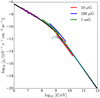 |
Fig. 1. Flux of IS CR electrons (black solid line) as a function of energy. Data: Voyager 1 (Cummings et al. 2016, solid purple squares) at low energies, AMS-02 (Aguilar et al. 2014, solid cyan circles) at high energies. The red, blue, and green thick lines show the energy range that mostly contributes to synchrotron emission in the frequency range of SKA for the values of the magnetic field strength listed in the legend (see Eq. (7)). The orange dashed line shows the CR electron-positron flux obtained from Galactic synchrotron emission (Orlando 2018). |
4. Density and magnetic field profiles
4.1. Density profile
A common feature of starless cores derived from millimetre(mm)-continuum observations is a central flattening in the density profile, with typical maximum densities of the order of 105 − 106 cm−3, reaching ∼2 × 107 cm−3 in the starless core L1544 (Keto & Caselli 2010). Various density profiles are used to reproduce observations of dense cores such as the Bonnor–Ebert sphere or softened power laws. In the following we adopt the latter profile as given by Tafalla et al. (2002)
where n0 is the central density, r0 the radius of the central flat region, and q the asymptotic slope.
Since the specific emissivity is a function of radius (Eq. (4)), in principle one should consider the attenuation of the IS CR electron flux due to energy losses (Padovani et al. 2009). However, the typical maximum H2 column densities of starless cores are of the order of 1023 cm−2; therefore only electrons with energies lower than 1 MeV can be stopped completely (Padovani et al. 2018). One should also take into account the fact that CRs follow helical trajectories along magnetic field lines, meaning that the effective column density passed through is larger than the corresponding line-of-sight column density (see e.g. Padovani et al. 2013). Strong bending of field lines is not expected in starless cores: assuming a poloidal field configuration, the effective column density is larger at most by a factor of approximately three (see Fig. 3 in Padovani & Galli 2011). We can then assume the effective column density and the line-of-sight column density to be the same. Besides, the minimum electron energy contributing to synchrotron emission for the range of frequencies and magnetic field strengths considered here is ∼100 MeV, corresponding to a value of the stopping range of the order of 6 × 1024 cm−2. Therefore, in Eq. (4), we can safely neglect the dependence of the CR electron flux on column density (i.e. on radius r).
4.2. Magnetic field strength profile
For the magnetic field strength we assume the relation
where B0 is the value of the magnetic field strength at the central density n0 and κ ∼ 0.5 − 0.7 is determined by observations (see e.g. Crutcher 2012). We use Eq. (9) as a local relation to obtain the strength of the magnetic field from the radial profile of n. While the choice of the density profile is unimportant for the attenuation of the CR electron flux (see Sect. 4.1), it has important consequences on the profile of B and, in turn, on the observed flux density. In the following section we compute the flux densities for different assumptions on the magnetic field profile. Synchrotron emissivity depends on B⊥ (see Eq. (4)). Here we simply assume B⊥ = π B/4 to account for a random orientation of the magnetic field with respect to the line of sight.
5. Modelling
5.1. General case
We consider three models of starless cores with outer radius R = 0.1 pc and central density n0 = 106 cm−3. We vary the radius of the central flat region and the asymptotic slope (the parameters r0 and q, respectively, in Eq. (8)) ranging from a relatively peaked profile (r0 = 14″, q = 2.5, model A) to an almost uniform profile (r0 = 75″, q = 4, model C), including an intermediate case (r0 = 30″, q = 2.5, model B). These profiles are similar to those used by Tafalla et al. (2002) to describe low-mass starless cores in the Taurus molecular cloud. The magnetic field strength is assumed equal to B0 = 50 μG at the centre of the core in all models, and we consider the two cases κ = 0.5 and 0.7 (Crutcher 2012). The left column of Fig. 2 shows both the density and magnetic field strength profiles of our models.
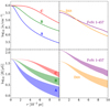 |
Fig. 2. Density and magnetic field strength profiles as a function of radius (upper and lower panels, respectively). Left column: models of starless cores described by Eq. (8), r0 = 14″, q = 2.5 (model A, solid blue line), r0 = 30″, q = 2.5 (model B, solid green line), and r0 = 75″, q = 4 (model C, solid red line). Right column: starless cores FeSt 1-457 (purple) and B68 (orange). Shaded areas in the lower panels encompass the curves obtained with Eq. (9) using κ = 0.5 and 0.7 for models A, B, C and B68 and κ = 0.68 and 0.88 for FeSt 1-457 (upper and lower boundary, respectively). |
We compute the specific intensity from Eqs. (4) and (5), assuming the CR electron flux given by Eq. (6). The observable quantity is the flux density S ν, obtained by integrating over the solid angle the specific intensity multiplied by the telescope pattern. The latter is assumed to be a Gaussian with beam full width at half maximum θ b = 300″ equal to the angular size of our starless core models at a distance of 140 pc (non-resolved source).
The upper row of Fig. 3 displays the flux density profiles at the five lowest frequencies of SKA1-Low for the three models and the sensitivity limits for one hour of integration. At higher frequencies, a source of 300″ is resolved, with consequent loss of flux. However, the total flux density can still be recovered by convolution with a larger beam.
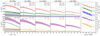 |
Fig. 3. Radial flux density profiles for the starless core models described in Sect. 5.1 (upper row) and for B68 and FeSt 1-457 (lower row, see Sect. 5.2). The observing frequency is shown in black at the top of each column, while numbers in the upper-right corner of each subplot represent the radius-averaged S/N for the two values of κ (0.5 and 0.7 for models A, B, C and B68, and 0.68 and 0.88 for FeSt 1-457, see Eq. (9)). Shaded areas encompass the curves obtained with Eq. (9) by using the two values of κ (see Fig. 2 for colour-coding). The telescope beam is shown in the leftmost column for models A, B, and C (dotted black line, 300″), B68 (short-dashed black line, 330″), and FeSt 1-457 (long-dashed black line, 284″). Hatched areas display SKA sensitivities for one hour of integration at different frequencies. The two panels on the right side show the flux density as a function of frequency. Empty (solid) circles refer to a S/N smaller (larger) than 3, respectively. The spectral index α is shown on the right of each curve. |
It is evident that what determines the maximum value of Sν is not only the maximum magnetic field strength, but also the integrated value of B along the line of sight, which, in turn, depends on the density profile: the shallower the density profile, the higher Sν is. As a consequence, for one hour of integration, a centrally peaked starless core such as model A is detectable with a signal-to-noise ratio (S/N) of about 2 only at frequencies higher than 158 MHz, whereas a less centrally concentrated core such as model B will be observable with S/N ≳ 3 at ν ≳ 114 MHz. For an almost uniform density profile such as model C, a S/N ≳ 2 is promptly reached at ν ≳ 60 MHz.
If the CR electron flux is proportional to E−p, the synchrotron flux density varies as Sν ∝ ν−α, where α = (p − 1)/2 is the spectral index (Rybicki & Lightman 1986). For our assumed CR electron flux, p → 1.3 at low energies and p → 3.2 at high energies (see Sect. 3), therefore α is expected to be intermediate between 0.2 and 1.1. In fact, our calculations show that α is about 0.6 in the frequency range 60 − 218 MHz (see the two rightmost panels in Fig. 3). Since in starless cores the IS CR electron flux is not attenuated, we expect the spectral index α ∼ 0.6 to be weakly dependent on density and magnetic field strength profiles at SKA1-Low frequencies as long as 10 μG ≲ B ≲ 1 mG.
The flux density depends weakly on the value of κ (from 10% in model C to 35% in model A, for κ ranging from 0.5 to 0.7), but it is strongly controlled by the strength of the magnetic field (Eq. (9)). For a power-law electron flux proportional to E−p the synchrotron emissivity is ϵν ∝ Bδ, where δ = (p + 1)/2 (see e.g. Rybicki & Lightman 1986). Since p varies between 1.3 and 3.2, we expect Sν to increase with the magnetic field strength with a dependence intermediate between δ = 1.2 and 2.1. Increasing the value of B0 from 10 μG to 1 mG in the case of the core model B we obtain the results shown in Fig. 4 (models A and C give similar results). In the frequency range 60 MHz − 218 MHz the flux density increases roughly in a power-law fashion with exponent ∼1.5 − 1.6. As a consequence, a larger value of B0 would make our modelled sources detectable with a shorter integration time.
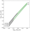 |
Fig. 4. Flux density at 60, 114, and 218 MHz (lower-left labels) as a function of magnetic field strength B0 for model B (see Sect. 5.1). Green shaded areas encompass the curves obtained with Eq. (9) by using κ = 0.5 and 0.7. Grey areas correspond to S/N < 3 and dashed lines are power-law fits of |

Finally, we note that in this work we consider typical outer radii of the order of 0.1 pc, but for bigger starless cores – especially with flat density profile – the flux density would be correspondingly larger than that shown in Fig. 3.
5.2. Magnetic field strength in FeSt 1-457 and B68
In this section we show the potential of SKA in observing two starless cores in the southern hemisphere: FeSt 1-457 (also known as Core 109 in the Pipe Nebula), and B68 in Ophiuchus. The density profiles of FeSt 1-457 and B68 are taken from Juárez et al. (2017) and Galli et al. (2002), respectively. According to Kandori et al. (2018), the magnetic field at the centre of FeSt 1-457 is B0 ∼ 132 μG decreasing with a slope κ = 0.78 ± 0.10, while the plane-of-sky magnetic field strength in B68 has been estimated by Kandori et al. (2009) as ∼20 μG. Since the total strength for a random field is about twice that measured along any direction (Shu et al. 1999), in the following we consider B0 = 40 μG for B68 in Eq. (9). The right column of Fig. 2 shows the density and the magnetic field strength profiles for these two starless cores.
Similarly to the three modelled cores in Sect. 5.1, we compute the flux density using a beam size equal to the angular size of B68 and FeSt 1-457 (330″ and 284″, respectively2). The results are shown in the lower row of Fig. 3. We find that a S/N larger than ∼2 is reached in one hour of integration at ν ≳ 82 MHz for B68, while FeSt 1-457 can be detected even at the lowest frequency ν = 60 MHz with S/N ≳ 3.
6. Conclusions
We explored the capability of SKA in detecting synchrotron emission from starless cores. This observing facility is very promising because it can provide robust constraints on the magnetic field strength, thus contributing to elucidate the role of magnetic fields in the star-formation process. Our main conclusions are as follows.
Thanks to the recent Voyager 1 measurements, combined with AMS-02 data and Galactic synchrotron emission, the flux of IS CR electrons is now well-known down to 3 MeV. Synchrotron emission is entirely dominated by primary CR electrons, while the contribution by secondary relativistic leptons is negligible.
For typical values of the magnetic field strength in starless cores (∼10 μG − 1 mG), synchrotron emission in the SKA1-Low and SKA1-Mid frequency bands is determined by electrons with energies between ∼100 MeV and ∼20 GeV. The stopping range at ∼100 MeV is of the order of 6 × 1024 cm−2, therefore the IS CR electron flux contributing to synchrotron emission is attenuated at H2 column densities much in excess of the typical column densities of starless cores.
The synchrotron radiation emitted by a starless core depends on the integrated line-of-sight value of the magnetic field strength, which, in turn, depends on the density profile. As a result, for the same maximum value of the magnetic field strength, a starless core with a shallow density profile shows a larger synchrotron flux density than a core with a peaked profile.
We modelled two starless cores in the southern hemisphere whose density profiles and typical magnetic field strengths are well-constrained by observations (B68 and FeSt 1-457) and we found that SKA will be able to detect synchrotron emission at 82 MHz ≲ ν ≲ 218 MHz reaching a S/N ∼ 2 − 5 and ∼10 − 23 in one hour of integration for B68 and FeSt 1-457, respectively; FeSt 1-457 can be detected even at the lowest frequency ν = 60 MHz with a S/N ≳ 3.
We found a typical spectral index α = (p − 1)/2 ∼ 0.6 intermediate between the values 0.2 and 1.1 resulting from the low- and high-energy asymptotic slopes of the primary CR electron flux (p → 1.3 and p → 3.2, respectively). Since in starless cores the IS CR electron flux is not attenuated by losses (although it can be modulated by self-generated turbulence; see Ivlev et al. 2018), we expect α ∼ 0.6 to be weakly dependent on density and magnetic field strength profiles at SKA1-Low frequencies.
Our study shows that SKA is a powerful instrument to constrain the strength of magnetic fields in molecular cloud cores. This facility and the proposed next-generation Very Large Array (ngVLA, Murphy et al. 2018) have the capability to shed light in the near future on the role of magnetic fields in the process of star formation.
We assume a radius R = 0.1 pc for both cores and a distance of 125 pc for B68 (de Geus et al. 1989) and 145 pc for FeSt 1-457 (Alves & Franco 2007).
Acknowledgments
We want to thank the referee for her/his helpful comments, which further improved the quality of this paper. MP acknowledges funding from the European Unions Horizon 2020 research and innovation programme under the Marie Skłodowska-Curie grant agreement No 664931. The authors thank Maite Beltrán, Riccardo Cesaroni, and Francesco Fontani for valuable discussions and the referee for useful suggestions and comments.
References
- Alves, F. O., & Franco, G. A. P. 2007, A&A, 470, 597 [NASA ADS] [CrossRef] [EDP Sciences] [Google Scholar]
- Alves, F. O., Franco, G. A. P., & Girart, J. M. 2008, A&A, 486, L13 [NASA ADS] [CrossRef] [EDP Sciences] [Google Scholar]
- Alves, F. O., Acosta-Pulido, J. A., Girart, J. M., Franco, G. A. P., & López, R. 2011, AJ, 142, 33 [NASA ADS] [CrossRef] [Google Scholar]
- Alves, F. O., Girart, J. M., Padovani, M., et al. 2018, A&A, 616, A56 [NASA ADS] [CrossRef] [EDP Sciences] [Google Scholar]
- Aguilar, M., Aisa, D., Alvino, A., et al. 2014, Phys. Rev. Lett., 113, 121102 [Google Scholar]
- Brown, R. L., & Marscher, A. P. 1977, ApJ, 212, 659 [NASA ADS] [CrossRef] [Google Scholar]
- Crutcher, R. M. 2012, ARA&A, 50, 29 [NASA ADS] [CrossRef] [Google Scholar]
- Crutcher, R. M., Troland, T. H., Lazareff, B., & Kazes, I. 1996, ApJ, 456, 217 [NASA ADS] [CrossRef] [Google Scholar]
- Cummings, A. C., Stone, E. C., Heikkila, B. C., et al. 2016, ApJ, 831, 18 [Google Scholar]
- de Geus, E. J., de Zeeuw, P. T., & Lub, J. 1989, A&A, 216, 44 [NASA ADS] [Google Scholar]
- Dickinson, C., Beck, R., Crocker, R., et al. 2015, Advancing Astrophysics withthe Square Kilometre Array (AASKA14), 102 [CrossRef] [Google Scholar]
- Galli, D., Walmsley, M., & Gonçalves, J. 2002, A&A, 394, 275 [NASA ADS] [CrossRef] [EDP Sciences] [Google Scholar]
- Girart, J. M., Beltrán, M. T., Zhang, Q., Rao, R., & Estalella, R. 2009, Science, 324, 1408 [NASA ADS] [CrossRef] [PubMed] [Google Scholar]
- Goldreich, P., & Kylafis, N. D. 1981, ApJ, 243, L75 [NASA ADS] [CrossRef] [Google Scholar]
- Hornby, J. M., & Williams, P. J. S. 1966, MNRAS, 131, 237 [NASA ADS] [CrossRef] [Google Scholar]
- Ivlev, A. V., Padovani, M., Galli, D., & Caselli, P. 2015, ApJ, 812, 135 [NASA ADS] [CrossRef] [Google Scholar]
- Ivlev, A. V., Dogiel, V. A., Chernyshov, D. O., et al. 2018, ApJ, 855, 23 [NASA ADS] [CrossRef] [Google Scholar]
- Jones, D. I., Protheroe, R. J., & Crocker, R. M. 2008, PASA, 25, 161 [NASA ADS] [CrossRef] [Google Scholar]
- Juárez, C., Girart, J. M., Frau, P., et al. 2017, A&A, 597, A74 [NASA ADS] [CrossRef] [EDP Sciences] [Google Scholar]
- Kandori, R., Tamura, M., Tatematsu, K.-I., et al. 2009, IAU Symp., 259, 107 [NASA ADS] [Google Scholar]
- Kandori, R., Tomisaka, K., Tamura, M., et al. 2018, ApJ, 865, 121 [NASA ADS] [CrossRef] [Google Scholar]
- Keto, E., & Caselli, P. 2010, MNRAS, 402, 1625 [NASA ADS] [CrossRef] [Google Scholar]
- Longair, M. S. 2011, High Energy Astrophysics (Cambridge: Cambridge University Press) [Google Scholar]
- Mac Low, M.-M., & Klessen, R. S. 2004, Rev. Mod. Phys., 76, 125 [NASA ADS] [CrossRef] [Google Scholar]
- Mouschovias, T. C., & Ciolek, G. E. 1999, in NATO Advanced Science Institutes(ASI) Ser. C, eds. C. J. Lada, & N. D. Kylafis, 540, 305 [Google Scholar]
- Munar-Adrover, P., Bosch-Ramon, V., Paredes, J. M., & Iwasawa, K. 2013, A&A, 559, A13 [NASA ADS] [CrossRef] [EDP Sciences] [Google Scholar]
- Murphy, E. J., Bolatto, A., Chatterjee, S., et al. 2018, ArXiv e-prints [arXiv:1810.07524] [Google Scholar]
- Orlando, E. 2018, MNRAS, 475, 2724 [NASA ADS] [CrossRef] [Google Scholar]
- Padovani, M., & Galli, D. 2011, A&A, 530, A109 [NASA ADS] [CrossRef] [EDP Sciences] [Google Scholar]
- Padovani, M., Galli, D., & Glassgold, A. E. 2009, A&A, 501, 619 [NASA ADS] [CrossRef] [EDP Sciences] [Google Scholar]
- Padovani, M., Hennebelle, P., & Galli, D. 2013, A&A, 560, A114 [NASA ADS] [CrossRef] [EDP Sciences] [Google Scholar]
- Padovani, M., Ivlev, A. V., Galli, D., & Caselli, P. 2018, A&A, 614, A111 [NASA ADS] [CrossRef] [EDP Sciences] [Google Scholar]
- Rybicki, G. B., & Lightman, A. P. 1986, Radiative Processes in Astrophysics (New Jersey: John Wiley & Sons), 400 [Google Scholar]
- Shu, F. H., Allen, A., Shang, H., Ostriker, E. C., & Li, Z.-Y. 1999, ed. C. J. Lada & N. D. Kylafis, 193 [Google Scholar]
- Strong, A. W., Orlando, E., & Jaffe, T. R. 2011, A&A, 534, A54 [NASA ADS] [CrossRef] [EDP Sciences] [Google Scholar]
- Tafalla, M., Myers, P. C., Caselli, P., Walmsley, C. M., & Comito, C. 2002, ApJ, 569, 815 [NASA ADS] [CrossRef] [Google Scholar]
- Vlemmings, W. H. T., Humphreys, E. M. L., & Franco-Hernández, R. 2011, ApJ, 728, 149 [NASA ADS] [CrossRef] [Google Scholar]
- Wolleben, M., & Reich, W. 2004, A&A, 427, 537 [NASA ADS] [CrossRef] [EDP Sciences] [Google Scholar]
All Figures
|
Fig. 1. Flux of IS CR electrons (black solid line) as a function of energy. Data: Voyager 1 (Cummings et al. 2016, solid purple squares) at low energies, AMS-02 (Aguilar et al. 2014, solid cyan circles) at high energies. The red, blue, and green thick lines show the energy range that mostly contributes to synchrotron emission in the frequency range of SKA for the values of the magnetic field strength listed in the legend (see Eq. (7)). The orange dashed line shows the CR electron-positron flux obtained from Galactic synchrotron emission (Orlando 2018). |
| In the text | |
|
Fig. 2. Density and magnetic field strength profiles as a function of radius (upper and lower panels, respectively). Left column: models of starless cores described by Eq. (8), r0 = 14″, q = 2.5 (model A, solid blue line), r0 = 30″, q = 2.5 (model B, solid green line), and r0 = 75″, q = 4 (model C, solid red line). Right column: starless cores FeSt 1-457 (purple) and B68 (orange). Shaded areas in the lower panels encompass the curves obtained with Eq. (9) using κ = 0.5 and 0.7 for models A, B, C and B68 and κ = 0.68 and 0.88 for FeSt 1-457 (upper and lower boundary, respectively). |
| In the text | |
|
Fig. 3. Radial flux density profiles for the starless core models described in Sect. 5.1 (upper row) and for B68 and FeSt 1-457 (lower row, see Sect. 5.2). The observing frequency is shown in black at the top of each column, while numbers in the upper-right corner of each subplot represent the radius-averaged S/N for the two values of κ (0.5 and 0.7 for models A, B, C and B68, and 0.68 and 0.88 for FeSt 1-457, see Eq. (9)). Shaded areas encompass the curves obtained with Eq. (9) by using the two values of κ (see Fig. 2 for colour-coding). The telescope beam is shown in the leftmost column for models A, B, and C (dotted black line, 300″), B68 (short-dashed black line, 330″), and FeSt 1-457 (long-dashed black line, 284″). Hatched areas display SKA sensitivities for one hour of integration at different frequencies. The two panels on the right side show the flux density as a function of frequency. Empty (solid) circles refer to a S/N smaller (larger) than 3, respectively. The spectral index α is shown on the right of each curve. |
| In the text | |
|
Fig. 4. Flux density at 60, 114, and 218 MHz (lower-left labels) as a function of magnetic field strength B0 for model B (see Sect. 5.1). Green shaded areas encompass the curves obtained with Eq. (9) by using κ = 0.5 and 0.7. Grey areas correspond to S/N < 3 and dashed lines are power-law fits of |
| In the text | |
Current usage metrics show cumulative count of Article Views (full-text article views including HTML views, PDF and ePub downloads, according to the available data) and Abstracts Views on Vision4Press platform.
Data correspond to usage on the plateform after 2015. The current usage metrics is available 48-96 hours after online publication and is updated daily on week days.
Initial download of the metrics may take a while.