| Issue |
A&A
Volume 620, December 2018
|
|
|---|---|---|
| Article Number | A161 | |
| Number of page(s) | 9 | |
| Section | Planets and planetary systems | |
| DOI | https://doi.org/10.1051/0004-6361/201833968 | |
| Published online | 12 December 2018 | |
High polarization degree of the continuum of comet 2P/Encke based on spectropolarimetric signals during its 2017 apparition
1
Department of Physics and Astronomy, Seoul National University,
1 Gwanak,
Seoul 08826,
Republic of Korea
e-mail: This email address is being protected from spambots. You need JavaScript enabled to view it.
; This email address is being protected from spambots. You need JavaScript enabled to view it.
2
Laboratory of Infrared High-Resolution Spectroscopy, Koyama Astronomical Observatory, Kyoto Sangyo University,
Motoyama Kamigamo,
Kita-ku,
Kyoto 603-8555, Japan
3
National Astronomical Observatory of Japan,
2-21-1 Osawa,
Mitaka,
Tokyo 181-8588, Japan
4
Hiroshima Astrophysical Science Center, Hiroshima University,
Kagamiyama 1-3-1,
Higashi-Hiroshima 739-8526,
Japan
5
Okayama Observatory, Kyoto University,
3037-5 Honjo,
Kamogata,
Asakuchi,
Okayama 719-0232, Japan
6
Ishigakijima Astronomical Observatory, National Astronomical Observatory of Japan,
1024-1 Arakawa,
Ishigaki,
Okinawa 907-0024, Japan
7
Nishi-Harima Astronomical Observatory, Center for Astronomy, University of Hyogo,
407-2, Nishigaichi, Sayo,
Hyogo 679-5313, Japan
8
Institute of Astronomy, Graduate School of Science, The University of Tokyo,
2-21-1 Osawa,
Mitaka,
Tokyo 181-0015, Japan
9
Tokyo Institute of Technology,
2-12-1 Ookayama,
Meguro,
Tokyo 152-8551, Japan
10
Faculty of Science, Department of Earth and Planetary Sciences, Hokkaido University,
Kita 10, Nishi 8,
Kita-ku,
Sapporo 060-0810, Japan
11
Graduate School of Science, Nagoya University,
Furo-cho,
Chikusa-ku,
Nagoya 464-8602, Japan
12
Graduate School of Science and Engineering, Kagoshima University,
1-21-35 Korimoto,
Kagoshima 890-0065,
Japan
13
Graduate School of Science and Engineering, Saitama University,
Simo-okubo 135,
Sakura-ku,
Saitama 338-8570, Japan
Received:
27
July
2018
Accepted:
3
October
2018
Abstract
Context. Spectropolarimetry is a powerful technique for investigating the physical properties of gas and solid materials in cometary comae without mutual contamination, but only a few spectropolarimetric studies have been conducted to extract each component.
Aims. We attempt to derive the continuum (i.e., scattered light from dust coma) polarization degree of comet 2P/Encke, free of the influence of molecular emissions. The target is unique in that its orbit is dynamically decoupled from Jupiter, like the main-belt asteroids, but it ejects gas and dust like ordinary comets.
Methods. We observed the comet using the Hiroshima Optical and Near-Infrared Camera attached to the Cassegrain focus of the 150 cm Kanata telescope on UT 2017 February 21 when the comet was at the solar phase angle of α = 75°.7.
Results. We find that the continuum polarization degree with respect to the scattering plane is Pcont, r = 33.8 ± 2.7% at the effective wavelength of 0.82 μm, which is significantly higher than those of cometary dust in a high-Pmax group at similar phase angles. Assuming that an ensemble polarimetric response of the dust of 2P/Encke as a function of phase angle is morphologically similar with those of other comets, its maximum polarization degree is estimated to Pmax ≳ 40% at αmax ≈ 100°. In addition, we obtain the polarization degrees of the C2 swan bands (0.51–0.56 μm), the NH2 α bands (0.62–0.69 μm), and the CN-red system (0.78–0.94 μm) in a range of 3–19%, which depend on the molecular species and rotational quantum numbers of each branch. The polarization vector is aligned nearly perpendicularly to the scattering plane with an average of 0°.4 over a wavelength range of 0.50–0.97 μm.
Conclusions. From the observational evidence, we conjecture that the high polarization degree of 2P/Encke might be attributable to a dominance of large dust particles around the nucleus, which have remained after frequent perihelion passages near the Sun.
Key words: comets: individual: 2P/Encke / methods: observational / techniques: polarimetric
© ESO 2018
1 Introduction
Comet 2P/Encke (hereafter 2P), which is a frequently observed comet because its orbital period is short (3.3 years), has a few distinctive characteristics, including its low dust cross-section with respect to the water production rate (4.27 × 10⁻²⁷; A’Hearn et al. 1995) and high dust-to-gas mass ratio (10–30; Reach et al. 2000). These characteristics suggest that large-size grains (up to ~0.1 m) dominate in the vicinity of the comet (Sarugaku et al. 2015). It is also known that 2P is dynamicallydecoupled from Jupiter (i.e., the Tisserand parameter with respect to Jupiter is TJ = 3.025), being an archetype of Encke-type comets, and it has been proposed that a long-term residence in the inner solar system results in this unique orbital property (Levison et al. 2006).
In general, the linear polarization of cometary dust particles can be exploited to constrain physical properties, such as their size and porosity (see, e.g., Kiselev et al. 2015). However, the large portion of gas emission signals in the coma of 2P can heavily depolarize the observed linear polarization degree of the dust component (Kiselev et al. 2004; Jockers et al. 2005). In this regard, spectropolarimetry can provide more reliable information about the properties of gas and dust, free of mutual contamination. The observation technique simultaneously provides a series of information on the polarization degrees (P) of the gas (Pgas) and dust components (Pcont) and of the position angle (θP) with respect to the normal vector of thescattering plane (θr). However, only a few studies in the literature have reported spectropolarimetric results of comets (Myers & Nordsieck 1984; Kiselev et al. 2013; Borisov et al. 2015).
Here, we report a new spectropolarimetric observation of 2P at a phase angle of α = 75°.7 in its inbound orbit. From our data analysis, we derive Pgas and Pcont values at 0.50–0.97 μm. In addition, wereport Pgas of the C2 swan band, NH2 α band, and CN-red system (A2 Π−X2Σ+) molecules in each branch. Based on the observational evidence, we discuss these polarimetric results in terms of the unique orbital property of 2P. We use the notations of PX for the linear polarization degrees and PX, r for the linear polarization degrees with respect to the scattering plane, where the subscript X specifies the continuum, gas, or molecular species.
2 Observations
We performed a spectropolarimetric (hereafter sppol) observation of 2P using the Hiroshima Optical and Near-Infrared Camera (HONIR) mounted on the Cassegrain focus of the 150 cm Kanata telescope at the Higashi-Hiroshima Observatory (HHO, 132°46′36′′ E, +34°22′39′′ N, 511.2 m), Japan, on UT 2017 February 21. Although we obtained optical and near-infrared data simultaneously with HONIR, we did not use the near-infrared data because 2P is not detected at this wavelength. In sppol mode, we employed a rotatable half-wave plate (HWP), a slit mask for five different fields (2.′′ 2 × 45.′′0 each), a Wollaston prism, and an optical grism (Akitaya et al. 2014). Accordingly, a single fits file consists of five pairs of sky spectra of ordinary and extraordinary light components at each HWP angle (in the sequence of 0°.0, 45°.0, 22°.5, and 67°.5 position angles to the fiducial point). The pixel and wavelength resolutions are 0.′′ 29 and R(= λ/Δλ) ~ 350, respectively (Akitaya et al. 2014).
We set the position angle of the slit parallel to the east-west direction. Initially, we positioned the nucleus on the center of the slit, but realized that the nuclear position was 8′′ off from the central slit at the last exposure because the non-sidereal tracking mode was not available for the telescope. We obtained data of a spectroscopic standard star, HR718 (B9III) (Hamuy et al. 1994), on the same night. The observed airmass of HR718 was slightly lower than that of 2P (airmass of 2.1 for HR718 and 2.7 for 2P), however, we used the standard star data for the flux calibration but not for the polarimetric calibration. We exploited the HONIR data reduction pipeline for the basic preprocessing and IRAF to extract the observed spectra. Detailed stages of P and the θP derivation for comets are described in Kuroda et al. (2015) and Kwon et al. (2017), and the standard sppol data reduction procedure is described in Kawabata et al. (1999). The observed polarimetric parameters were corrected for instrumental effects (i.e., for the instrumental polarization, the polarization efficiency, and for the correction angle of the HONIR sppol mode) at Stokes Q(λ) and U(λ) levels, usingroutinely checked calibration data provided by H. Akitaya (a coauthor of the paper who developed the instrument). Instrumental polarization (Figs. 12c and 13 at Akitaya et al. 2014) stably varies within ± 0.1% over the OPT filter (0.5–1.0 μm), thus we considered that its influence on our results of 2P would be negligible. For the polarization efficiency and position angle corrections, (Figs. 15a and b, respectively, in Akitaya et al. 2014), which are smoothly varying functions over the OPT filter domain, we fit the data using the least-squares methods to interpolate them in the wavelength resolution of HONIR (Δ λ ~ 0.002 μm). All polarimetric quantities discussed in the following sections are corrected for these instrumental effects.
In addition to the sppol observation, we conducted contemporaneous multi-band imaging observations with the 105 cm telescope at the Ishigakijima Astronomical Observatory (IAO), Japan, on UT 2017 February 19 and with the Okayama Astrophysical Observatory’s (OAO) 50 cm telescope on UT 2017 February 21 to monitor the dust coma morphology and brightness. We employed the MITSuME imaging system (to obtain the g′, RC, and IC bands simultaneously; it consists of 1024 × 1024 CCD chips with a 24.0-μm pixel pitch) at these observatories (Kotani et al. 2005). The g′, RC, and IC filters transmit the light at λc = 0.48, 0.66, and 0.80 μm with Δλ = 0.13, 0.12, and 0.16 μm, respectively, where λc and Δλ denote the central wavelengths of each filter and their full width at half-maximum (FWHM). We also made a spectroscopic observation using the MALLS spectrograph1 attached to the 2 m telescope at the Nishi-Harima Astronomical Observatory (NHAO) of University of Hyogo, Japan, on UT 2017 February 19 to examine the strengths of molecular emissions with respect to the dust continuum. The observed raw data were preprocessed in a standard manner using dark (for the IAO data) and bias (for the HONIR data) and flat frames. We transformed the pixel coordinates into celestial coordinates using WCSTools (Mink 1997) and conducted flux calibration using field stars listed in the UCAC-3 catalog (Zacharias et al. 2010). We tabulate the detailed observation geometry and instrumental setup in Table 1.
3 Results
3.1 General outlines
Figure 1a shows the dust intensity map on UT 2017 February 19 taken with the IAO telescope after we subtracted the gas intensity from the observed intensity. We chose this image not only because there is no obvious change in the appearance and magnitude between the data on February 19 at IAO and February 21 at OAO, but also because the signal-to-noise ratio (S/N) of the IAO data is better than that of the OAO data. To extract dust signals from the observed signals, we used the simple manipulation of multiband images described by Ishiguro et al. (2016), assuming that IC band has little gas contamination than g′ band. We first made the gas intensity map by subtracting the IC-band image from the g′-band image, which in turn was subtracted from the RC-band image, adjusting sky levels as approximately zero. The remaining intensity in RC -band image would most likely represent the distribution of the 2P dust component. The dust cloud, which is elongated nearly normal to the antisolar direction, has 14.9 ± 0.2 mag in the RC-band within 5.′′ 8 in radius (i.e., the physical distance of ≈4200 km from the photocenter at the comet position). Compared to the predicted apparent nucleus magnitude of 18.3 mag at the observed geometry (the phase coefficient of β = 0.06 mag deg−1 and absolute magnitude of mR (1,1,0) = 15.2 ± 0.5 mag are assumed; Fernández et al. 2000), our photometry indicates that the observed signal is largely dominated by the dust coma, with negligible amount of nucleus signal. We also note possible contamination of large dust particles in the 2P dust trail (ejected before the last perihelion passage) within the aperture we employed. However, we were unable to detect any background dust structure extending along the negative velocity vector (Fig. 1a) because the dust trail is fainter than the coma surface brightness. Although it is possible that part of the dust signals within the aperture might come from the old dust trail of 2P, we consider that most of the dust intensity comes from the fresh dust tail of 2P.
Figure 2 shows the results of the sppol observation. We do not show the spectrum taken at NHAO because there is no noticeable difference between NHAO and HHO data. It consists of a weak continuum (overlaid by the signals from coma dust) and line emissions (Fig. 2a). Assuming an optically thin coma for all species used here, the total sum of the two strongest C2 bands (i.e., C2(0,0) at λ = 0.51 μm and C2 (3,4) at λ = 0.55 μm) is (3.1 ± 0.1) × 10−11 erg cm−2 s−1. The flux of the strongest CN(1, 0) red band is (3.2 ± 0.2) × 10−12 erg cm−2 s−1 μm−1, and the total sum of the NH2 bands shows a weak signal of (3.5 ± 0.4) × 10−13 erg cm−2 s−1. We note that the total flux of the above C2 emissions at λ < 0.55 μm could be overestimated because they are blended with NH2 α band emissions. Similarly, the fluxes of NH2 could be slightly overestimated because of the blending with oxygen emission (O(1D)) at λ = 0.63 μm and C2 bands at λ = 0.54–0.62 μm.
The flux of C2 (0,0) (Δν = 0) band (~2.0 × 10⁻¹¹ erg cm−2 s−1) allows us to conduct an order-of-magnitude estimate on the gas production rate (Q ; mol s−1). From the parameters in Table II of A’Hearn et al. (1995), we derived the g-factor (luminosity per molecule, i.e., fluorescence efficiency), scale length, and daughter lifetime of C2 scaled by the observing geometry (rh = 0.54 au). To compensate for flux loss caused by a limited area of the slit we employed, we estimated the dimensionless Haser correction factor from the volume fraction of total coma contained within the circular aperture of radius 2.′′02, which covers the equivalent area of 2.′′ 2 × 5.′′8 of the rectangular aperture employed in this study. By substituting the scaled parameters into Eq. (1) from Venkataramani et al. (2016), we obtained log(Q
 ) = 27.65. However, we note again that these band fluxes might not be accurate because of the airmass mismatch between the standard star and 2P, but they do explain the inverse relationship with the polarization degrees, as shown below.
Observational geometry and instrument settings.
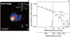 |
Fig. 1 Dust intensity map (panel a) and its radial profile (panel b) after we subtracted the gas components from the observed signals on UT 2017 February 19 by IAO/MITSuME. (a) The photocenter of 2P is markedas a red cross. The contours on 2P are spaced linearly down to one-fifth of the central brightness level (i.e., 95, 70, 45, and 20% flux with regard to the peak flux). The negative velocity (− v) and antisolar (r⊙) vectors projected on the celestial plane are shown as solid and dashed arrows, respectively. North is up and east is left. “S” letters in the bottom right corner denote the remnants of background stars. Panel b: The surface brightness profile of the near-nuclear coma with respect to the radial distance. We binned the radial distance logarithmically over 1.′′ 0–13.′′0, and averaged the data points at intervals of 0.′′5 radial distance each. All brightness points are normalized at the innermost point (0.′′ 2 from the photocenter). The upper solid and lower dashed lines exhibit gradients of −1 and − 1.5, which are typical of cometary dust expanding with initial ejection speed under the solar radiation field (Jewitt & Meach 1987). The blue vertical line at 5.′′ 8 denotes the apertureradius we used. |
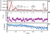 |
Fig. 2 Flux (panel a), P (panel b), and θr (panel c) of 2P observed on UT 2017 February 21 by HHO/HONIR as a function of wavelength. In panel a, we name the branches of discernible line emissions. The red line is a median-smoothed line of the original black points within the size of wavelength resolution. In panel b, the binned-average P is calculated within a rectangle region of 2.′′2 × 5.′′8. We mark the analyzed emission lines with the vertical lines in panels a and b. In panel c, the horizontal red line denotes the average θr of 0°.4. |
3.2 Continuum polarization
At first glance, the observed P has an inverse relationship with the line emission flux (Figs. 2a and b). The local minima are found around the emission peaks (the verticallines). Figure 2b shows an almost flat continuum spectrum. From this data, we obtain the polarimetric color of −1.0 ± 0.9 % (1000Å)−1.
To derive an average Pcont (i.e., for the dust), we extracted the continuum signals, avoiding the polarimetric data at the wavelengths of the line emissions described in the catalog of Brown et al. (1996). Wavelengths of the continua used to estimate the average Pcont are 0.680–0.690, 0.720–0.730, 0.760–0.770, 0.845–0.870, 0.880–0.910, 0.930–0.935, and 0.945–0.970 μm. We then transformed Pcont into the polarization degree of the continuum with respect to the normal vector of the scattering plane (Pcont, r) as follows:
 (1)
(1)
and
 (2)
(2)
where ϕ is the position angle of the scattering plane (the plane of Sun-comet-observer), whose sign satisfies the condition of 0° ≤ (ϕ ± 90°) ≤ 180° (Chernova et al. 1993). The ϕ value at the time of this sppol observation was 56°.3. From Eqs. (1)–(2), we obtain Pcont, r = 33.8 ± 2.7% at λ = 0.68–0.97 μm at the effective wavelength of λeff = 0.82 μm. θr is shown in Fig. 2c. The polarization vector is aligned nearly perpendicularly to the scattering plane (i.e., the average of θr = 0°.4 over the region of 0.50–0.97 μm), but exhibits a downward trend as the wavelength increases (which would be a real feature because we corrected for the wavelength dependence in θr using data of strongly polarized stars, but we know no plausible physical reason for the dust property).
As indicated by the dust image (Fig. 1a), whose flux is ~22.5 times brighter than the predicted one of the 2P nucleus, the dust continuum measured in this study should be dominated by the coma dust. This assumption can also be supported by comparison with Jewitt (2004), who performed the narrowband imaging polarimetry on/around the nucleus: (i) the aperture size in this study (1550 km × 4080 km) is 1.5–4.0 times larger than the coverage of his data, and (ii) the heliocentric distance in this study (0.54 au) is nearly twice smaller than those of Jewitt (2004). This suggests more significant contribution of dust coma with respect to the nucleus as a result of theincreasing solar incident flux.
To derive the phase angle dependence of Pcont, r, we searched the published narrowband data of 2P to minimize the influence of the gas emission, but found no consistent dataset whose radial distance matches ours. The physical distances from the nucleus we cover are 2–3, and 4 times larger than the data in Jewitt (2004; λeff = 0.526 μm; open diamonds in Fig. 3a) and Jockers et al. (2005; λeff = 0.642 μm; open squares in Fig. 3a), respectively. Meanwhile, for the broadband data in Böehnhardt et al. (2008; filled triangles in Fig. 3a) obtained at the large heliocentric distance (rh = 2.7–2.1 au), most of the polarized signals they obtained came from the bare nucleus, so that it could hardly be included in the line with our study as the dust signals.
Our Pcont, r (33.8 ± 2.7%) at α = 75°.7 is already significantly higher than the average Pcont, r of the dust-rich comets (the thin solid line in Fig. 3a). Thus, instead of compiling the published data, assuming that an ensemble polarimetric response of the dust of 2P as a function of phase angle is morphologically similar with those of other comets (i.e., a bell-shaped curve having a minimum Pmin at α ~ 10°, a maximum Pmax at α ~ 100°, and an inversion angle α0 at α ~ 15°–20°), we multiplied the average Pcont, r distribution of dust-rich comets by the constant (1.5) to match our sppol data.
We fit the published narrowband data using the empirical phase function written in Penttilä et al. (2005):
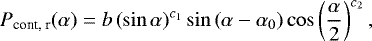 (3)
(3)
where b, c1, c2, and α0 are constants to characterize the profile. For comparison, we show the profiles of high- and low-Pmax comets in the archive data (Kiselev et al. 2006) (λeff = 0.67 μm) in Fig. 3a, whose parameters are determined to be b = 33.25 ± 1.66%, c1 = 0.85 ± 0.04, c2 = 0.39 ± 0.02, and α0 = 21°.90 ± 1°.10 for the high-Pmax comets and b = 17.78 ± 0.89%, c1 = 0.61 ± 0.03, c2 = 0.14 ± 0.01, and α0 = 21°.90 ± 1°.10 for the low-Pmax ones (Kwon et al. 2017). As a result, we derive the maximum polarization degree of Pmax ≳ 40% at the phase angle of αmax ≈ 100° (thick red solid line in Fig. 3a). This Pmax value is approximately 12% higher than the average Pmax of high-Pmax comets (≈28%) defined by Levasseur-Regourd et al. (1996). We note that the expected Pmax roughly coincides with the dust coma polarization values of the published data of 2P at high phase angles, ensuring that the large Pcont, r is a common nature of dust from the comet.
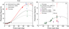 |
Fig. 3 Phase angle dependence of Pcont, r (panel a) and Pgas, r (panel b). In panel a, the thick solid line shows the trend of the 2P continuum component weighted by the data errors. The solid and dashed lines denote the average trends of high- and low-Pmax comets, respectively. The filled symbols denote the data used in fitting, and open symbols are the excluded ones. The solid curve in panel b denotes the empirical phase function of fluorescence lines (Öhman 1941). The molecules analyzed in this study are expressed as stars. The meanings of the different symbols are given in the legend at the top left panel. Open stars of C2 bands and of CN(3,1) are enlarged to avoid mutual overlapping. |
3.3 Molecule polarization
For the molecular polarization analysis, we excluded two NH2 regions at the central wavelengths of λc = 0.60 and 0.63 μm to prevent the leverage of foreign gas (O(1D) and C2). The analyzed regions are marked by the vertical lines in Fig. 2b, whose central wavelengths are λc = 0.51, and 0.55 μm for C2 Swan bands, λc = 0.66, 0.70, and 0.74 μm for NH2 α bands, and λc = 0.79, 0.81, 0.92 and 0.94 μm for CN bands (the so-called CN-red system). We tabulate the detailed information of molecular bands we analyzed and their polarization degrees in Table 2. We first subtracted the continuum signals determined in Sect. 3.2 and derived the polarization degrees of line emissions in the same manner as Pcont. In this process, we confirmed that molecules have inherent nonzero Pgas values at the observed phase angle. Figure 4 zooms in on the corresponding regions to show each analyzed molecule in panels a–i.
To identify the wavelengths and intensities of molecular emissions, we calculated the distribution of fluorescent lines in optical wavelengths (0.4–1.0 μm) at the sppol observing geometry of 2P, and we used the fluorescence excitation models of C2 (Shinnaka et al. 2010), NH2 (Kawakita et al. 2000), and CN (Shinnaka et al. 2017). In the NH2 model, we assumed the fluorescence equilibrium condition and fixed an ortho-to-para abundance ratio of 3.2, which is a typical value found in comets (Shinnaka et al. 2016). In the C2 and CN models, we assumed that the rotational energy levels in the ground vibronic state are maintained to the Boltzmann distribution for a given excitation temperature. The given temperatures for the C2 and CN models are 4000 K (a typical value found in comets; Rousselot et al. 2012) and 289 K (close to the fluorescence equilibrium condition; Shinnaka et al. 2017), respectively.
Figure 4 shows the polarization degrees of the gas components (i.e., Pgas), where the solid lines are the weighted means of Pgas within the wavelength resolution (Δλ ~ 0.002 μm). We overplot the corresponding branches for the C2 and CN transitions at the top of the figures. C2 bands are attributed to both P and R branches, and most of CN-red bands are dominated by Q branches (more details are described in Sect. 4.1). On average, we obtain Pgas = 8.0 ± 1.0% and Pgas = 7.2 ± 0.4% for the (0,0) and (3,4) transitions of the C2 swan band, respectively, and Pgas = 8.4 ± 1.3%, Pgas = 3.8 ± 1.2%, Pgas = 5.8 ± 0.7%, and Pgas = 18.5 ± 3.1% for each CN-red (2,0), (3,1), (1,0), and (2,1) transition. For NH2 α bands, due to their feeble fluxes embedded in the continuum signal, we zoom in on the very near regions of the line centers and obtain Pgas = 4.0 ± 1.0%, Pgas = 3.7 ± 0.5%, and Pgas = 7.0 ± 0.8% for (0,7,0), (0,6,0), and (0,10,0) transitions, respectively.
Detailed information of the analyzed molecular bands and their polarization degrees.
4 Discussion
4.1 Polarization of C2, NH2, and CN-red molecules
Öhman (1941) suggested two principal mechanisms of comet polarization: polarized light by dust continuum (Pcont), and by fluorescent molecule emissions (Pgas). The latter follows a empirical phase function:
 (4)
(4)
where p90 denotes the maximum polarization value at α = 90°, which was derived as 7.7% (a limiting value of Pgas with a high rotational quantum number of diatomic molecules that was theoretically determined from the 1 Π −1Σ transition of the Zeeman splitting in the magnetic field (Mrozowski 1936). Since then, phase angle dependence of Pgas has been mainly discussed in terms of the observed Pgas values beingconsistent or inconsistent with the profile of Eq. (4) (hereafter the reference Pgas profile).
Le Borgne et al. (1987) compared the observed Pgas of C2 (λc = 0.51 μm), CN-violet (λc = 0.38 μm), and OH (λc = 0.31 μm) molecules of comet 1P/Halley and 103P/Hartley-Good via narrowband imaging polarimetry to the reference Pgas profile in Öhman (1941; Fig. 3b). They found that Pgas values of C2 and CN-violet follow the reference Pgas profile well, whereas those of the OH band were nearly five times smaller than the curve. They could not find any explanation for this deviation. Sen et al. (1989) also measured the Pgas of CN-violet, C3, CO+, C2, and H2 O+ molecules of comet 1P/Halley via narrowband imaging polarimetry. They found agreement for CN-violet, C3, and C2, but deviations of CO+ and H2 O+ from the reference Pgas profile. Recently, Borisov et al. (2015) measured the Pgas of C2 of C/2013 R1 (Lovejoy) via spectropolarimetry and confirmed its distribution along the fluorescent phase curve. For the Pgas of NH2 α bands, Kiselev et al. (2004) used the differential imaging method to extract the gas signal and derived Pgas of (mainly) NH2(0, 7, 0) as ≈3% for 2P at α = 80°.5 and for C/1999 J3 (LINEAR) at α = 61°.6. In the same manner, Jockers et al. (2005) derived Pgas of NH2(0, 7, 0) of 2P during its 2003 apparition as ≈7% at α = 90° (purple squares and diamonds in Fig. 3b). The Pgas of the CN-red system has not yet been reported in refereed journals.
We compare our Pgas values with the published data in Fig. 3b. Green, purple, and red present the Pgas values of C2, NH2 α, and CN-redsystem molecules, respectively. The stars were obtained by us, and the squares and diamonds are quoted from the references described in the top left corner. The reference Pgas profile described by Eq. (4) with p90 = 7.7% is drawn asthe black solid line. Figure 3b confirms that our Pgas of C2 of 2P follows the curve well in terms of measurement accuracy, whereas the Pgas of NH2 and CN-red molecules deviate greatly. Overall, NH2 molecules have lower Pgas values thanthose found by Öhman (1941). By contrast, the Pgas values of CN-red molecules present fairly large variations of Pgas for each transition of the molecule.
We conjecture that the phase angle distribution of Pgas would be related to the type of molecular transitions. Le Borgne & Crovisier (1987) proposed a possible range of Pgas, as determined by the types of transitional behaviors, complementing the theories of Mrozowski (1936) and Öhman (1941), who considered a single case of polarization by fluorescent molecular emissions. For molecules, a possible range of Pgas can be determined by the relative dominance among the P, Q, and R branches of molecular transition (Le Borgne & Crovisier 1987). The P and R branches are induced by the fluorescence excitation of Δ J = +1 and Δ J = −1, respectively, whereas the resonant Q-branch results from the transition of Δ J = 0, where J is the total angular momentum quantum number. A possible range of Pgas induced by the fluorescence is Pgas = 0–7.7%, whose limiting value agrees with the P90 = 7.7% (Le Borgne & Crovisier 1987). Meanwhile, the dynamic range of Pgas induced by resonant Q branch is much wider (i.e., −14% to +19% without consideration of hyperfine structure of molecules) than those of the P and R branches.
Our fluorescence excitation model (see Sect. 3.3) shows the relative contribution of each molecular branch to reproduce the observed band emissions of 2P. Two strong C2 swan bands of 2P (Figs. 4a and b) are mainly triggered by the fluorescent P and R branches, while the intensity of the resonant Q branch therein is much weaker (i.e., ≲10-3) than the intensities of P and R. By contrast, most of the CN-red bands (A2 Π − X2Σ-) spanning the wavelengths of 0.78–0.94 μm (Figs. 4c–e) are caused largely by Q branches, and the relative influence of P and R in these intervals is negligible as <10-2 times. In thecase of CN(2,1) at λ ~ 0.94 μm (Fig. 4f), the dominant transition occurs by the R branch. However, both (1) the comparable intensities of the Q and R branches (i.e., 10-1 < flux(Q/R) < 1) for this band and (2) the weak continuum-subtracted signal make it hard to interpret this result clearly. For NH2, its transitions have systematic differences with the cases of diatomic C2 and CN, so we must consider three vibrational (symmetric, bending, and asymmetric) modes induced by its structural form of XY2 (X and Y denote different atomic species). For now, we have no theoretical interpretation to explain the systematically lower Pgas of the NH2 α band than C2 at the given phase angle, but we can infer that our result for NH2 is consistentwith previous molecular observations.
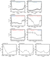 |
Fig. 4 Panels a and b: Pgas of C2 (0,0) and C2 (3,4), respectively. Panels c–f: Pgas of the CN(2,0), CN(3,1), CN(1,0), and CN(2,1) transitions, panels g–i: those of the NH2 (0,7,0), (0,6,0), and (0,10,0) α bands, respectively. Solid lines are median-smoothed within the wavelength resolution (i.e., Δ λ ~ 0.002 μm), and the background gray dashed lines present the modeled distributions of line emissions under the fluorescence equilibrium at the observation geometry of 2P. The right axis of panels a–i was arbitrarily scaled for visibility. More detailed information is described in the text. |
4.2 Polarimetric anomaly of the 2P continuum
It has been conventionally suggested that two polarimetric groups of comets exist, that is, the high-Pmax and low-Pmax groups (Levasseur-Regourd et al. 1996). The former tends to be dust rich, and the latter is mainly gas rich. Recently, Kwon et al. (2017) noted that C/2013 US10 (Catalina), which was originally categorized in the low-Pmax group, can be classified into the high-Pmax group after subtracting the gas influence. This evidence suggests that the polarimetric signals in the low-Pmax group might be largely contaminated by the gas emissions and that the two polarimetric classes do not necessarily result from the difference of dust physical properties. From the research, it is also inferred that cometary dust particles have a unified polarimetric property and show a phase angle dependence similar to that of high-Pmax comets. It is important, however, to note that the 2P continuum data do not coincide with the majority of comets (Fig. 3a), even though the gas contaminations were adequately subtracted. As mentioned above, our flux data contain ambiguity due to the airmass mismatch between our target and the standard star. However, sppol data provide more reliable results because we derive them by comparing the ordinary and extraordinary components of light taken simultaneously using the Wollaston prism, which eliminates the ambiguity of atmospheric influence without flux calibration. Thus, the large polarization is probably attributable to an inherent scattering property of 2P dust and the nuclear surface. However, what causes the 2P continuum to deviate from a population of normal comets?
Pcont,r tends to increase via Rayleigh scattering as the abundance of small (<submicron) dust particles increases (Bohren & Huffman 1983). It is likely that the fragility of dust can increase under solar heat due to the evaporation of the gluing volatile matrix. This effect would result in the disaggregation of dust receding from the nucleus and would generate smaller constituent particles in the coma, as proposed in previous polarimetric research of 2P (Jewitt 2004). Similarly, scattered light by neutral gas components can enhance the Pcont,r. However, the enhancement by small particles is probably not the case of large Pcont,r for 2P. We do not find any evidence of a small dust population that extended along the antisolar direction of the extra-solar radiation pressure. In Fig. 1a, the dust cloud was elongated nearly perpendicularly to both the antisolar and negative orbital velocity vectors, most likely because of a population of compact large grains ejected from an active region via a jet of 2P (Sekanina 1988). Our radial profile of the dust intensity map (Fig. 1b) also indicates the absence of significant disintegration of outward dust particles within the aperture radius we considered (the vertical line at 5.′′ 8 from the photocenter). All brightness points are located in between the slopes of −1 and −1.5, which are typical of cometary dust expanding with initial ejection speed under the solar radiation field (Jewitt & Meach 1987), supporting our discussion point. In addition, our sppol data do not show an obvious increase in Pcont,r at shorter wavelengths, where the contribution of small Rayleigh scattering particles should be dominant in the signal to increase the polarization degree. We note, however, that our result does not refute the hypothesis of disaggregation in a smaller radial scale. Because the spatial resolution of Jewitt (2004; 0.′′ 22 per pixel) is nearly one-third of Fig. 1a (0.′′72 per pixel), with 2–3 times smaller aperture size, we are unable to verify the hypothesis of disaggregation of porous in the innermost of dust coma.
There are several possibilities to increase Pcont. The so-called Umow effect indicates that Pmax has an inverse correlation with the geometric albedo, which implies that multiple scattering among individual particles or constituent monomers in dust aggregates reduces Pmax (see, e.g., Zubko et al. 2011). However, the geometric albedo of the 2P dust particles (0.01–0.04 for the large dust grain, Sarugaku et al. 2015, and 0.03–0.07 for the nucleus, Fernández et al. 2000) shows albedos that are typical of general cometary dust (~0.04; Kolokolova et al. 2004) and nuclei (0.02–0.06; Lamy et al. 2004), although their results include large errors in the albedo measurements.
We speculate that the unique dust size distribution of 2P would lead to a larger Pcont,r compared to those of other comets. As mentioned in Sect. 1, the dominance of large grains (i.e., a paucity of small grains) from2P has been suggested by the observations of the featureless spectra (Lisse et al. 2004) and the unique morphology of the dust cloud with the dust trail structure (Reach et al. 2000; Epifani et al. 2001; Ishiguro et al. 2007; Sarugaku et al. 2015). Such a dust trail should be produced by large compact dust grains that are less sensitive to the solar radiation pressure. It is thus probable that the large opaque compact particles suppress multiple scattering in a single particle such that the surface single-scattering signals are magnified to increase the Pmax values. The polarimetric measurement in the laboratory indicate that large dust-free rocks tend to retain higher Pmax values than submillimeter-size grains do, although the experiment demonstrated that planetary surfaces where inter-particle multiple scattering should occur, unlike an optically thin cometary dust cloud (Geake & Dollfus 1986).
2P has the shortest orbital period of 3.3 yr of the Jupiter-Family comets, and it has a small perihelion distance (q ~ 0.3 au), which means that 2P can be an object more susceptible to solar radiation (e.g., photon pressure and solar heat) than other comets. It is also suggested that 2P resides in the inner solar system for a long time to be decoupled with Jupiter gravity (Levison et al. 2006). Taking account of the unique orbital properties as well as our polarimetric results, we conjecture that small dust grains have been lost from the surface and the circumnucleus environment by the gas drag force and from the dust mantle layer, which consists of mainly fall-back boulder-size rocks. The sintering effect by solar heat near the perihelion may also contribute to create coherent large dust particles on/around the surface of 2P, as suggested for 1566 Icarus and 3200 Phaethon (Ishiguro et al. 2017; Ito et al. 2018). Additionally, the packing effect of fluffy particles, which is caused by a sublimation of volatile materials on dust grains, can reduce the empty space in the conglomerated fluffy dust, removing multiple scattering within particles (Mukai & Fechtig 1983). Although the real physical mechanism for the large Pcont of the comet is not yet clear, such an unusual environment could be related to the polarimetric anomaly.
Acknowledgements
We thank the referee, H., Boehnhardt, whose constructive comments improved our manuscript. The observational data were obtained under the framework of a campaign program in the Optical and Infrared Synergetic Telescopes for Education and Research (OISTER). This work at Seoul National University was supported by a National Research Foundation of Korea (NRF) grant funded by the Korean Government (MEST), No. 2015R1D1A1A01060025. Y.G.K is supported by the Global Ph.D. Fellowship Program through the NRF funded by the Ministry of Education (NRF-2015H1A2A1034260). Y.S. was supported by Grant-in-Aid for JSPS Fellows Grant No. 15J10864.
References
- A’Hearn, M. F., Millis, R. L., Schleicher, D., Osip, D. J., & Birch, P. V. 1995, Icarus, 118, 223 [NASA ADS] [CrossRef] [Google Scholar]
- Akitaya, H., Moritani, Y., Ui, T., et al. 2014, Proc SPIE, 9147, 91474O [Google Scholar]
- Bohren, C. F.,& Huffman, D. R. 1983, Absorption and Scattering of Light by Small Particles (New York: Wiley) [Google Scholar]
- Böehnhardt, H., Tozzi, G. P., Bagnulo, S., et al. 2008, A&A, 489, 1337 [NASA ADS] [CrossRef] [EDP Sciences] [Google Scholar]
- Borisov, G., Bagnulo, S., Nikolov, P., & Bonev, T. 2015, Planet. Space Sci., 118, 187 [NASA ADS] [CrossRef] [Google Scholar]
- Brown, M. E., Bouchez, A. H., Spinrad, H., & Johns-Krull, C. M. 1996, AJ, 112, 1197 [NASA ADS] [CrossRef] [Google Scholar]
- Chernova, G. P., Kiselev, N. N., & Jockers, K. 1993, Icarus, 103, 144 [NASA ADS] [CrossRef] [Google Scholar]
- Epifani, E., Colangeli, L., Fulle, M., et al. 2001, Icarus, 149, 339 [NASA ADS] [CrossRef] [Google Scholar]
- Fernández, Y. R., Lisse, C. M., Käufl, H. U., et al. 2000, Icarus, 147, 145 [NASA ADS] [CrossRef] [Google Scholar]
- Geake, J. E., & Dollfus, A. 1986, MNRAS, 218, 75 [NASA ADS] [Google Scholar]
- Hamuy, M., Suntzeff, N. B., Heathcote, S. R., et al. 1994, PASP, 106, 566 [NASA ADS] [CrossRef] [Google Scholar]
- Ishiguro, M., Sarugaku, Y., Ueno, M., et al. 2007, Icarus, 189, 169 [NASA ADS] [CrossRef] [Google Scholar]
- Ishiguro, M., Kuroda, D., Hanayama, H., et al. 2016, ApJ, 152, 169 [Google Scholar]
- Ishiguro, M., Kuroda, D., Watanabe, M., et al. 2017, AJ, 154, 180 [NASA ADS] [CrossRef] [Google Scholar]
- Ito, T., Ishiguro, M., Arai, T., et al. 2018, Nat. Commun., 9, 2486 [Google Scholar]
- Jewitt, D. 2004, AJ, 128, 3061 [NASA ADS] [CrossRef] [Google Scholar]
- Jewitt, D., & Meech, K. 1987, ApJ, 317, 992 [NASA ADS] [CrossRef] [Google Scholar]
- Jockers, K., Kiselev, N., Bonev, T., et al. 2005, A&A, 441, 773 [NASA ADS] [CrossRef] [EDP Sciences] [Google Scholar]
- Kawakita, H., Kazuya, A., & Tetsuya, K. 2000, PASJ, 52, 925 [NASA ADS] [CrossRef] [Google Scholar]
- Kawabata, K. S., Okazaki, A., Akitaya, H., et al. 1999, PASP, 111, 898 [NASA ADS] [CrossRef] [Google Scholar]
- Kiselev, N., Jockers, K., & Bonev, T. 2004, Icarus, 168, 385 [NASA ADS] [CrossRef] [Google Scholar]
- Kiselev, N., Velichko, S., Jockers, K., Rosenbush, V., & Kikuchi, S. 2006, NASA Planetary Data System, Database of Comet Polarimetry (DOCP), EAR-C-COMPIL-5-COMET-POLARIMETRY-V1.0 [Google Scholar]
- Kiselev, N. N., Rosenbush, V. K., Afanasiev, V. L., et al. 2013, Earth Planets Space, 65, 1151 [NASA ADS] [CrossRef] [Google Scholar]
- Kiselev, N., Rosenbush, V., Kolokolova, L., & Levasseur-Regourd, A.-Ch. 2015, Polarization of Stars and Planetary Systems, (Cambridge: Cambridge University Press), 379 [CrossRef] [Google Scholar]
- Kolokolova, L., Hanner, M. S., Levasseur-Regourd, A.-C., & Gustafson, B. Å. S. 2004, Comets II, 577 [NASA ADS] [Google Scholar]
- Kossacki, K. J., Kömle, N. I., Kargl, G., & Steiner, G. 1994, Planet. Space Sci. 42, 383 [NASA ADS] [CrossRef] [Google Scholar]
- Kotani, T., Kawai, N., Yanagisawa, K., et al. 2005, NCimC, 28, 755 [Google Scholar]
- Kuroda, D., Ishiguro, M., Watanabe, M., et al. 2015, ApJ, 814, 156 [NASA ADS] [CrossRef] [Google Scholar]
- Kwon, Y. G., Ishiguro, M., Kuroda, D., et al. 2017, AJ, 154, 173 [NASA ADS] [CrossRef] [Google Scholar]
- Lamy, P. L., Toth, I., Fernandez, Y. R., & Weaver, H. A. 2004, Comets II, 223 [NASA ADS] [Google Scholar]
- Le Borgne, J. F., & Crovisier, J. 1987, ESA SP, 278, 171 [NASA ADS] [Google Scholar]
- Le Borgne, J. F., Leroy, J. L., & Arnaud, J. 1987, A&A, 173, 180 [NASA ADS] [Google Scholar]
- Levasseur-Regourd, A. C., Hadamcik, E., & Renard, J. B. 1996, A&A, 313, 327 [NASA ADS] [Google Scholar]
- Levison, H. F., Terrell, D., Wiegert, P. A., Dones, L., & Duncan, M. J. 2006, Icarus, 182, 161 [NASA ADS] [CrossRef] [Google Scholar]
- Lisse, C. M., Fernández, Y. R., A’Hearn, M. F., et al. 2004, Icarus, 171, 444 [NASA ADS] [CrossRef] [Google Scholar]
- Mink, D. J. 1997, ADASS, 125, 249 [NASA ADS] [Google Scholar]
- Mrozowski, S. 1936, Acta Phys. Pol. 5, 85 [Google Scholar]
- Mukai, T., & Fechtig, H. 1983, Planet. Space Sci., 31, 655 [NASA ADS] [CrossRef] [Google Scholar]
- Myers, R. V., & Nordsieck, K. H. 1984, Icarus, 58, 431 [NASA ADS] [CrossRef] [Google Scholar]
- Öhman Y. 1941, StoAn, 13, 11 [NASA ADS] [Google Scholar]
- Penttilä, A., Lumme, K., Hadamcik, E., & Levasseur-Regourd, A.-C. 2005, A&A, 432, 1081 [NASA ADS] [CrossRef] [EDP Sciences] [Google Scholar]
- Reach, W. T., Sykes, M. V., Lien, D., & Davies, J. K. 2000, Icarus, 148, 80 [NASA ADS] [CrossRef] [Google Scholar]
- Rousselot, P., Jehin, E., Manfroid, J., & Hutsemákers, D. 2012, A&A, 545, A24 [NASA ADS] [CrossRef] [EDP Sciences] [Google Scholar]
- Sarugaku, Y., Ishiguro, M., Ueno, M., Usui, F., & Reach, W. T. 2015, ApJ, 804, 127 [NASA ADS] [CrossRef] [Google Scholar]
- Sekanina, Z. 1988, AJ, 96, 1455 [Google Scholar]
- Sen, A. K., Joshi, U. C., & Deshpande, M. R. 1989, A&A, 217, 307 [NASA ADS] [Google Scholar]
- Shinnaka, Y., Kawakita, H., Kobayashi, H., & Kanda, Y. 2010, PASJ, 62, 263 [NASA ADS] [CrossRef] [Google Scholar]
- Shinnaka, Y., Kawakita, H., Jehin, E. et al. 2016, MNRAS, 462, 195 [Google Scholar]
- Shinnaka, Y., Kawakita, H., Kondo, S., et al. 2017, AJ, 154, 45 [NASA ADS] [CrossRef] [Google Scholar]
- Venkataramani, K., Ghetiya, S., Ganesh, S., et al. 2016, MNRAS, 463, 2137 [NASA ADS] [CrossRef] [Google Scholar]
- Zacharias, N., Finch, C., Girard, T., et al. 2010, AJ, 139, 2184 [NASA ADS] [CrossRef] [Google Scholar]
- Zubko, E., Videen, G., Shkuratov, Y., Muinonen, K., & Yamamoto, T. 2011, Icarus, 212, 403 [NASA ADS] [CrossRef] [Google Scholar]
All Tables
Detailed information of the analyzed molecular bands and their polarization degrees.
All Figures
|
Fig. 1 Dust intensity map (panel a) and its radial profile (panel b) after we subtracted the gas components from the observed signals on UT 2017 February 19 by IAO/MITSuME. (a) The photocenter of 2P is markedas a red cross. The contours on 2P are spaced linearly down to one-fifth of the central brightness level (i.e., 95, 70, 45, and 20% flux with regard to the peak flux). The negative velocity (− v) and antisolar (r⊙) vectors projected on the celestial plane are shown as solid and dashed arrows, respectively. North is up and east is left. “S” letters in the bottom right corner denote the remnants of background stars. Panel b: The surface brightness profile of the near-nuclear coma with respect to the radial distance. We binned the radial distance logarithmically over 1.′′ 0–13.′′0, and averaged the data points at intervals of 0.′′5 radial distance each. All brightness points are normalized at the innermost point (0.′′ 2 from the photocenter). The upper solid and lower dashed lines exhibit gradients of −1 and − 1.5, which are typical of cometary dust expanding with initial ejection speed under the solar radiation field (Jewitt & Meach 1987). The blue vertical line at 5.′′ 8 denotes the apertureradius we used. |
| In the text | |
|
Fig. 2 Flux (panel a), P (panel b), and θr (panel c) of 2P observed on UT 2017 February 21 by HHO/HONIR as a function of wavelength. In panel a, we name the branches of discernible line emissions. The red line is a median-smoothed line of the original black points within the size of wavelength resolution. In panel b, the binned-average P is calculated within a rectangle region of 2.′′2 × 5.′′8. We mark the analyzed emission lines with the vertical lines in panels a and b. In panel c, the horizontal red line denotes the average θr of 0°.4. |
| In the text | |
|
Fig. 3 Phase angle dependence of Pcont, r (panel a) and Pgas, r (panel b). In panel a, the thick solid line shows the trend of the 2P continuum component weighted by the data errors. The solid and dashed lines denote the average trends of high- and low-Pmax comets, respectively. The filled symbols denote the data used in fitting, and open symbols are the excluded ones. The solid curve in panel b denotes the empirical phase function of fluorescence lines (Öhman 1941). The molecules analyzed in this study are expressed as stars. The meanings of the different symbols are given in the legend at the top left panel. Open stars of C2 bands and of CN(3,1) are enlarged to avoid mutual overlapping. |
| In the text | |
|
Fig. 4 Panels a and b: Pgas of C2 (0,0) and C2 (3,4), respectively. Panels c–f: Pgas of the CN(2,0), CN(3,1), CN(1,0), and CN(2,1) transitions, panels g–i: those of the NH2 (0,7,0), (0,6,0), and (0,10,0) α bands, respectively. Solid lines are median-smoothed within the wavelength resolution (i.e., Δ λ ~ 0.002 μm), and the background gray dashed lines present the modeled distributions of line emissions under the fluorescence equilibrium at the observation geometry of 2P. The right axis of panels a–i was arbitrarily scaled for visibility. More detailed information is described in the text. |
| In the text | |
Current usage metrics show cumulative count of Article Views (full-text article views including HTML views, PDF and ePub downloads, according to the available data) and Abstracts Views on Vision4Press platform.
Data correspond to usage on the plateform after 2015. The current usage metrics is available 48-96 hours after online publication and is updated daily on week days.
Initial download of the metrics may take a while.