| Issue |
A&A
Volume 620, December 2018
|
|
|---|---|---|
| Article Number | A73 | |
| Number of page(s) | 16 | |
| Section | The Sun | |
| DOI | https://doi.org/10.1051/0004-6361/201833648 | |
| Published online | 04 December 2018 | |
Real-time, multiframe, blind deconvolution of solar images
1
Instituto de Astrofísica de Canarias, 38205
La Laguna, Tenerife, Spain
e-mail: This email address is being protected from spambots. You need JavaScript enabled to view it.
2
Departamento de Astrofísica, Universidad de La Laguna, 38205
La Laguna, Tenerife, Spain
3
Institute for Solar Physics, Dept. of Astronomy, Stockholm University, Albanova University Center, 10691
Stockholm, Sweden
4
Kiepenheuer-Institut für Sonnenphysik, 79104
Freiburg, Germany
Received:
15
June
2018
Accepted:
24
September
2018
Abstract
The quality of images of the Sun obtained from the ground are severely limited by the perturbing effect of the Earth’s turbulent atmosphere. The post-facto correction of the images to compensate for the presence of the atmosphere require the combination of high-order adaptive optics techniques, fast measurements to freeze the turbulent atmosphere, and very time-consuming blind deconvolution algorithms. Under mild seeing conditions, blind deconvolution algorithms can produce images of astonishing quality. They can be very competitive with those obtained from space, with the huge advantage of the flexibility of the instrumentation thanks to the direct access to the telescope. In this contribution we make use of deep learning techniques to significantly accelerate the blind deconvolution process and produce corrected images at a peak rate of ∼100 images per second. We present two different architectures that produce excellent image corrections with noise suppression while maintaining the photometric properties of the images. As a consequence, polarimetric signals can be obtained with standard polarimetric modulation without any significant artifact. With the expected improvements in computer hardware and algorithms, we anticipate that on-site real-time correction of solar images will be possible in the near future.
Key words: techniques: image processing / methods: data analysis / Sun: atmosphere
© ESO 2018
1. Introduction
Arguably the largest difficulty to face when observing the Sun from Earth is the perturbing effect of the atmosphere. The turbulent variations of the index of refraction at different layers of the atmosphere produce distortions in the images that severely reduce the quality of the observations. Perhaps the most obvious way of avoiding this effect is to move the telescope to space. Examples of this are Hinode (Suematsu et al. 2008) and/or Sunrise (Solanki et al. 2010), which allowed us to have images of the solar surface with high quality for the whole duration of the missions. Nevertheless, ground-based telescopes hold many advantages. Instruments can be modified and tuned online, which can help reach unprecedented levels of detail in the investigated solar signals. Additionally, ground-based telescopes can be made with significantly larger apertures. Large telescopes are complicated and heavy machines that are better operated at ground level.
Many efforts have been put into compensating for the perturbing effect of the atmosphere. A very successful frontline is the development of active and adaptive optics that measure the wavefront perturbations at a high time cadence and correct it using deformable optical elements. Working at very high frequencies (up to a few kHz), current adaptive optics (AO) systems can very effectively correct for the turbulent layers closer to the telescope, remarkably enhancing the quality of the science data. Even with such corrections, turbulence at higher layers, which typically produce a spatially variant image motion, remains uncorrected. To this end, multi-conjugate AO (MCAO) systems based on several deformable mirrors that are conjugate with the turbulence layer at different heights have been proposed. The first tests for solar observations (Schmidt et al. 2017) have demonstrated that this approach is able to correct a much larger field of view (FOV).
Another frontline is the development of a-posteriori image-correction algorithms. These methods are also routinely applied even in observations carried out with AO systems. The reason is that the corrections carried out by the deformable mirrors are often incomplete and there is still a non-negligible atmospheric residual in the observations. Under the assumption of the linear theory of image formation, the perturbing effect of the atmosphere can be compensated for using optimization methods. In such an approach, the observed image I is computed from the real object, O as
 (1)
(1)
where P is a linear operator that characterizes the instantaneous point spread function (PSF) of the atmosphere at every spatial position of the image. The previous equation can often be simplified inside small FOVs (the so-called anisoplanatic patch, which share the same PSF) to the convolution
 (2)
(2)
Since both the real image and the PSF are unknown, almost all methods that are currently in use or have potential to be developed belong to the class of blind (or semi-blind) inversion schemes, in which both the solar image, O, and the PSF, P, need to be simultaneously obtained. Only in few cases do we find examples of non-blind inversion in which the wavefront is measured and used to infer the PSF. Blind inversion problems are always very ill-defined and the solution strongly depends on the assumption of priors. It is therefore necessary to add extra information to better condition the problem, and some avenues have been tried in solar physics. Arguably the first method used in the field was the speckle technique (Labeyrie 1970; von der Lühe 1993), in which many short-exposure images (where the atmospheric seeing can be considered to be frozen) are obtained. This method can be understood as a semi-blind inversion, in which partial statistical information about the wavefront is estimated from models (we note that it remains to be checked whether the speckle method can be posed as an optimization of a merit function, like the rest of the inversion schemes discussed in this section). They are later combined to estimate the amplitude and phase of the Fourier transform of the original object. A second method widely used in solar physics is that of phase diversity (Paxman et al. 1992; Löfdahl & Scharmer 1994; Löfdahl et al. 1998). Under the assumption of uncorrelated Gaussian noise, Paxman et al. (1992) demonstrated that a proper likelihood function can be obtained in which the image O does not explicitly appear and one only needs to optimize for the wavefront. One of the most widespread applications of this approach is that in which two images (typically one in focus and the other one defocused) are used to jointly estimate the wavefront and the original object. To this end, the wavefront (usually defined on a circular or annular pupil) is developed in a suitable orthogonal basis (usually Zernike polynomials or Karhunen-Loeve modes) and the coefficients are obtained by maximizing the likelihood. Once the PSF is estimated, the final image can be obtained with a standard non-blind deconvolution. This method has been recently used with success for correcting the data obtained with the Imaging Magnetograph eXperiment (IMaX; Martínez Pillet et al. 2011) onboard Sunrise (Solanki et al. 2010).
Perhaps the most successful method so far, and the one achieving the best corrections, is multi-object multiframe blind deconvolution (MOMFBD; van Noort et al. 2005). This method consists of a maximum-likelihood solution to the deconvolution problem which uses, arguably in order of importance: i) phase diversity, ii) many frames of the same object observed with different wavefront perturbations, and iii) many different objects (monochromatic images at different wavelengths) observed simultaneously with exactly the same wavefront perturbation. A method to use all of them was already derived by Löfdahl (2002), who also implemented a computer program taking into account the first two. It was later extended to many objects by van Noort et al. (2005). The enormous redundancy of the multi-object and multiframe scheme introduces strong constraints into the maximum-likelihood solution and produces excellent deconvolved images.
The fundamental problem of the majority of a-posteriori image-processing algorithms is of a computational character, both in terms of computing power and memory. Of special relevance is the case of MOMFBD, in which large supercomputers working for many hours are needed to deconvolve the observed data. This is a very limiting factor that will become even more severe with the advent of 4-m class telescopes in solar physics. In this contribution we make use of end-to-end deep learning solutions for deconvolving multiframe bursts of solar images. The resulting schemes can be deployed on Graphical Processing Units (GPUs) and can produce deconvolved images almost in real-time. This opens up the possibility of on-the-fly blind deconvolution in current and future telescopes. The methods that we present here can be applied to produce science-ready data or can be used to help the observer to have a better understanding of what can be expected prior to the standard data reduction and MOMFBD deconvolution.
2. Neural network architectures
The success of machine learning approaches based on deep neural networks (DNN) is beyond doubt. Apart from the enormous amount of applications1 in computer vision, natural language processing, and other fields, we also find applications in astrophysics such as the classification of galactic morphologies (Huertas-Company et al. 2015) or the development of generative models to help constrain the deconvolution of images of galaxies (Schawinski et al. 2017). In the field of solar physics, this approach has allowed us to infer horizontal velocity fields from consecutive continuum images (Asensio Ramos et al. 2017) and also to simultaneously deconvolve and super-resolve images (Díaz Baso & Asensio Ramos 2018) from the synoptic telescope Helioseismic and Magnetic Imager (HMI; Scherrer et al. 2012) onboard the Solar Dynamics Observatory (SDO; Pesnell et al. 2012).
In this paper we use multiframe (video) correction methods which, in the deep learning literature, are treated using fundamentally two approaches. The first one is to fix the number of input frames and use them as channels in a standard convolution neural network (CNN). The output of the CNN is the corrected frame, taking into account all the spatial information encoded in the degraded frames. To process a larger number of frames, one applies the DNN in batches until all frames are exhausted. However, fixing the number of frames in the burst can be seen as a limiting factor and an approach that works the same irrespective of the number of frames in the bursts would be preferable. This is of particular relevance in the special case when adding more frames can have a large impact on the final quality of the corrected image.
The second approach is to use a DNN with some type of recurrency, so that frames are processed in order. New frames are injected into the network and a corrected version of the image is obtained at the output. Introducing new frames into the input will slowly improve the quality of the output. This procedure can be iterated until a good enough final image is obtained.
In this paper we have explored the two options. The case in which we fix the number of frames of the input is an end-to-end approach based on an encoder-decoder network that we describe in Sect. 2.1. The case of a recurrent neural network is based on the very flexible strategy followed by Wieschollek et al. (2017) and is explained in Sect. 2.2. Although the quality of the output is similar, there are pros and cons for each one of the architectures, which we point out in the following. For many of the technical details, we refer the reader to our previous works (Asensio Ramos et al. 2017; Díaz Baso & Asensio Ramos 2018).
2.1. Encoder-decoder architecture
The architecture that we use in the encoder-decoder network is displayed in Fig. 1. The input I contains a fixed number of input frames (commonly known as channels) of size N × N. We use seven in our case. The input is marked as a light red block. Then, several standard differentiable operations (illustrated as colored blocks) are applied in sequence. These blocks are organized in eight super-blocks with different image sizes (labeled with the numbers above the super-blocks).
 |
Fig. 1. Architecture of the encoder-decoder deconvolution neural network. The network is composed of the input and eight super-blocks, each one made of a different number of blocks. The meanings of colors for the blocks are described in Sect. 2.1. The specific details for each block is described in Table 1. The numbers above the blocks label the super-blocks. |
In summary, the network follows a standard encoder-decoder architecture. In the encoder phase the spatial size of the images is reduced while increasing the number of channels. In the decoder phase, the original size is recovered by upsampling. Each colored block has the following meaning:
-
Red blocks are input blocks, containing all seven frames of the burst.
-
Yellow blocks are output blocks, containing just a single deconvolved frame (channel), which we label
 .
. -
Gray blocks are standard convolutional blocks made of (in this order): a batch normalization layer (BN; Ioffe & Szegedy 2015), a rectified linear unit (ReLU; Nair & Hinton 2010) as activation function, and a convolutional layer with kernel size and depth defined in Table 1. To keep the size of the images unchanged, the images are padded in the borders using reflection padding.
Table 1.Architecture of encoder-decoder network.
-
Dark-blue blocks are convolution blocks like the previous ones, but using a stride of two during convolution (in other words, the convolution is carried out by sliding the kernel on the input in steps of two pixels). This reduces the size of the output by a factor of two.
-
Orange blocks are upsampling convolutional blocks made of (in order) BN, ReLU, upsampling by a factor of two using a nearest-neighbor interpolation, and finally a convolutional layer. We prefer upsampling+convolution as a substitute for the standard transpose convolution for upsampling given that the latter can easily produce checkerboard artifacts2.
For the specific details of our implementation, we refer to Table 1, where each layer is indicated as Cs, i, with s referring to the super-block and i to the specific block inside each super-block.
Our architecture also contains many shortcut connections displayed as arrows connecting two non-consecutive blocks in Fig. 1. These connections (He et al. 2016) simply add the input to the output, producing an important acceleration in the training by avoiding the effect of vanishing gradients3. The encoder-decoder architecture has at least two advantages as compared with the fully convolutional architectures that kept the size of the images throughout the network and that we used in our previous works (Asensio Ramos et al. 2017; Díaz Baso & Asensio Ramos 2018). The first is that the computing time is reduced because convolutions are applied over increasingly smaller images during the encoder phase. The second is that small kernels (like the 3 × 3 kernels that we use in this work) can produce much larger receptive fields (they affect much larger regions in the input image after multiple convolutions) thanks to the reduction in size of the images through the encoder phase4. On the contrary, the training is often more difficult because the network needs to recognize how to generate high spatial frequency in the decoder phase from the combination of information in different channels.
2.2. Recurrent architecture
The recurrent architecture we have used is displayed in Fig. 2, and is essentially the one used by Wieschollek et al. (2017) but with a few minor modifications. It consists of a single encoder-decoder network very similar to our encoder-decoder architecture. This network takes as input two frames, I(i) and I(i + 1), and produces as output a deconvolved frame  (we remind the reader that we use the “hat” to denote corrected frames). The output frame is used, together with a new frame of the burst, to produce a new estimation of the corrected frame. This is iterated until the frames of the burst are exhausted. The architecture also propagates some information internally from one block to the next. The internal structure of each deconvolution block of the upper panel of Fig. 2 is displayed in the lower panel of the same figure. Some of these blocks have already been described above, while the new ones have the following properties:
 |
Fig. 2. Upper panel: end-to-end deconvolution process, where the gray blocks are the deconvolution blocks described in the lower panel. Lower panel: internal architecture of each deconvolution block. Colors for the blocks are described in Sect. 2.2, with the specific details for each block being described in Table 2. |
Architecture of recurrent network.
-
Purple blocks are similar to standard convolutional blocks but using kernels of spatial size 1 × 1. Therefore, they compute a weighted average along the channel dimension.
-
Green blocks carry out the concatenation of two inputs with the same spatial dimensions and the same number of channels, producing an output with twice the number of channels. The memory from previous frames is passed along the green arrows to subsequent iterations and merged in these green blocks. Specifically, we extract features from blocks 4, 5, and 6, and blend them again in the same blocks for the next iteration. These connections are obviously not operative for the first iteration of the deconvolution block.
The reader can note that our architecture differs from that used by Wieschollek et al. (2017) in two minor points. The first one is the size of some of the kernels. The second is that we have used upsampling+convolution as a substitute for the standard transpose convolution. We also note that, apart from the possibility of injecting an arbitrary number n of frames into the recurrent architecture, this network also allows for the output of n − 1 corrected frames, which can later be used to improve the signal-to-noise ratio.
3. Training
3.1. Training dataset
We have trained both DNNs5 using two datasets observed with the CRisp Imaging SpectroPolarimeter (CRISP) instrument at the Swedish 1-m Solar Telescope (SST) on the Observatorio del Roque de los Muchachos (Spain). We have tried to use datasets that cover a broad variety of solar regions, from quiet Sun to more active regions. The training set was obtained in fairly good average seeing conditions. However, there were some significant seeing variations, especially at the beginning of the series. Therefore, we think that the training set contains a broad representation of good to average seeing conditions. One of the datasets corresponds to a quiet Sun region, observed on 19 September 2016 from 10:03 to 10:04 UT. The other one is a region of flux emergence, observed on the same day from 09:30 to 10:00. The data used for training are spectral scans on the Fe I doublet at 6301–6302 Å, containing 15 wavelength points, and the Ca II line at 8542 Å, containing 21 wavelength points. The observations are recorded in four modulated polarization states, which allow us to reconstruct the full Stokes vector. CRISP includes dual beam polarimetry to minimize seeing-induced cross-talk (see, e.g., Casini et al. 2012). The image acquisition is performed in such a way that the four polarization states are interleaved sequentially until seven acquisitions are acquired in each state. The exposure time per acquisition is ∼17.35 ms and the pixel size is 0.059′. Additionally, strictly simultaneous wide band (WB) images are acquired with the narrow band (NB) images, which are used for the deconvolution process.
The images are reduced following the standard procedure (de la Cruz Rodríguez et al. 2015) that includes dark current subtraction, flat-field correction, and subpixel image alignment between the two NB cameras and the WB camera. The bursts of seven images and the simultaneous WB images are used by the MOMFBD technique to recover a deconvolved final image. The MOMFBD code applies a Fourier filter to the reconstructed images that suppresses frequencies above the diffraction limit of the telescope (or from a practical point of view, above the noise limit), as described in van Noort et al. (2005). We use these images as the output of our training set. Two additional datasets of the same region obtained on the same day are used as a validation set to check for over-fitting during the training.
A total of 𝒩 = 80 000 patches of 88 × 88 pixels are randomly extracted from the bursts of seven images and from the final deconvolved image. They are also randomly extracted from the spectral positions and from the polarimetric modulation states. The size of 88 pixels allows us to reduce the size of the image three times in the encoder phase, always obtaining images of integer size. Given that the network is fully convolutional, it can be safely applied to images of arbitrary size. However, we point out that in order to recover an output of the same size as the input, the number of pixels in both directions has to be an integer multiple of 8. We also apply an augmenting strategy that consists of randomly flipping the patches horizontally and vertically. This improves the generalization capabilities of the neural networks.
3.2. Optimization
The previous neural networks are trained by optimizing a loss function that measures how far the outputs of the network are when compared with the target images. The encoder-decoder network is trained by minimizing the loss function
 (3)
(3)
which measures the sum over the full training dataset of 𝒩 patches of the ℓ2 distance between the deconvolved frames obtained at the output of the network,  , and the one deconvolved with the MOMFBD algorithm, ID(i). We note that i loops indistinctly over the randomly extracted 88 × 88 patches, the CRISP spectral scanning positions, and the four modulation states. To summarize, we use the scalar L as a measurement of the quality of the prediction of the neural network. We have found very good results using this simple loss function and did not witness a significant smearing as reported elsewhere (e.g., Ledig et al. 2016; Schawinski et al. 2017). The loss function is optimized with the Adam stochastic gradient descent type algorithm (Kingma & Ba 2014) with a learning rate of 3 × 10⁻⁴. The network is trained for 180 epochs with a batch size of 1206. The number of trainable parameters is 3.15 million. Each epoch lasts for roughly 6 min on an NVIDIA Titan X GPU, so the total training time is close to 19 h. We checked during training that the network is not overtraining (adapting to the training dataset and not correctly generalizing) by computing the loss on a validation set of images.
The recurrent neural network is more difficult to train because of the presence of recurrent connections, which slow down the back-propagation. Nevertheless, the residual connections and the Adam optimizer are enough to reach a good convergence. Following Wieschollek et al. (2017), the training is carried out by optimizing the loss function
 (4)
(4)
where n is the number of frames included during training (seven in our case, but this can be applied for any number of frames). This loss function forces intermediate deconvolved frames to approximate to the final target. To summarize, this scalar loss function measures the mismatch between the target image and the prediction produced by the recurrent neural network after each new frame is injected. The number of trainable parameters in this case is 4.02 million. Each epoch lasts for roughly 30 min on an NVIDIA P100 GPU, so the total training time is close to 2.5 days.
3.3. Validation
The results of the network applied to some patches of the validation set for the encoder-decoder architecture are displayed in Fig. 3. The first column shows the target image given by MOMFBD. The second column gives the output of the deep neural network. For comparison, we display the best and worst individual short-exposure frames (in terms of the root-mean-square contrast) in the last two columns and the time average of the burst in the third column. It is obvious that the neural network approach is able to extract high-frequency information from the burst of images, even though this information is not present in each individual raw frame.
 |
Fig. 3. Selection of patches from the training set. First column: target MOMFBD corrected patch. Second column: output to the encoder-decoder network when converged. Third column: average of the seven frames of the burst, while the last two columns are two of these individual frames. |
4. Results
4.1. Testing
Once both neural networks are trained, we apply them to datasets different to those used for training and validation. Given the fully convolutional character of both architectures, one can apply it to frames of arbitrary size (integer multiple of 8 to end up with input and outputs of the same size). Additionally, this very same fully convolutional character allows the network to transparently deal with spatially variant seeing conditions. The correction carried out for each pixel in the input image is done as if a potentially different PSF is perturbing it. For this reason, there is no gain in correcting images by mosaicking and one can input the full frames into the networks. The only practical limitation is in terms of memory, especially relevant for GPUs with their limited amount of memory. One needs to make sure that the parameters of the networks, together with the intermediate results of each step in the network, can be allocated in memory. We had no problem in deconvolving 1k × 1k images in an NVIDIA Titan X GPU with 12 GB of memory. In any case, images that do not fit in the memory can be corrected by mosaicking with some overlap and then stitching the patches using, for instance, the median value for the overlapping regions. In terms of computing time, a Titan X GPU is able to deconvolve images of 1k × 1k in less than 5 ms for the encoder-decoder architecture and of the order of 50 ms for the recurrent architecture.
Another interesting side effect of our learning-based approach to solar image deconvolution is that no WB channel is, a priori, necessary for the deconvolution. The WB channel, taken in strict simultaneity with the monochromatic images of the spectral scan and the polarimetric modulation, is used by the MOMFBD algorithm to help in the deconvolution. Once the networks are trained, this channel is no longer needed, which largely facilitates the instrumental setup. As a caveat, this is probably an exaggeration because the WB channel is used in the current CRISP instrumental setup for other purposes like image alignment.
In terms of performance, Figs. 4 and 5 show the comparison between the encoder-decoder and the recurrent networks and the target MOMFBD image for two different monochromatic images, representative of the general behavior. The left column shows the image obtained after the MOMFBD processing, with the upper row displaying an image in the continuum and the lower row an image in the core of the lines. In general, both networks produce a very similar output, with very detailed fine structure. One can argue that there is an apparent lack of sharpness in the output of the networks as compared with the MOMFBD image. It is more obvious in the filamentary structure in the upper panel of Fig. 4 and especially in the lower panel of Fig. 5. Fibrils in the core of the Ca II 8542 Å line are slightly more well defined in the MOMFBD image than in the outputs of the networks. However, we think that part of the sharpness is a consequence of the residual noise in the MOMFBD image, which appears as a strongly spatially correlated structure, more visible in the upper panel of Fig. 5. It is clear that both networks are perfectly able to filter out this noise (that is present in the training set). The random selection of patches for building the training set has the desirable consequence of breaking a significant part of the spatial correlation of the noise in the MOMFBD images. Consequently, the networks are unable to reproduce it and, as a result, partially filter it out from the predictions.
 |
Fig. 4. First column: images reconstructed with MOMFBD. Central column: output of the recurrent network. Right column: results for the encoder-decoder network. Upper row: image in the continuum around 6302 Å. Lower panel: image in the core of the line in a different part of the FOV. |
These properties are better quantified by analyzing the spatial frequencies in the neural network predictions as compared with those of the original frames and the MOMFBD images. The left column of Fig. 6 shows the case of the continuum at 6302 Å in a quiet Sun region, while we display the results for the core of the 8542 Å line in the right column of the same figure. The upper panel shows one of the original frames, the middle panel displays the frame corrected with the recurrent network, while the lower panel shows the azimuthally averaged power spectrum for the original and reconstructed frame with all the methods considered in this work. The general behavior of the power spectrum is fundamentally the same for a large variety of observed frames and regions, so the discussion can be made with only these two. Concerning the photospheric data, the individual frames present a clear lack of power on spatial periods of ∼3 and ∼30 pixels, which correspond to those mainly affected by the seeing. Both the recurrent end encoder-decoder architectures are able to recover these spatial frequencies and increase their power, imitating what is done with MOMFBD. Additionally, noise appearing on small scales is efficiently dampened by all image reconstruction methods. Concerning the chromospheric data, we witness a small general increase in the power for almost all frequencies, except in the very small scales with periods below two pixels where noise starts to dominate over the signal.
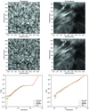 |
Fig. 6. Top panels: single raw image from the burst. Middle panels: reconstructed frames with the recurrent network. Lower panels: azimuthally averaged Fourier power spectra of the images. Left column: results from the continuum image at 6302 Å. Right column: results at the core of the 8542 Å line. All power spectra have been normalized to the value at the largest period (but not shown in the plot because it is outside the displayed range). |
To show the ability of the recurrent network to correct individual frames, we show in Fig. 7 the case of observations of the leading sunspot of AR12326 observed on 19 April 2015 using CRISP mounted on the SST. Two spectral regions were recorded sequentially: 6173 Å (with the well-known Fe I line) and 8542 Å, acquiring four modulation states in 20 and 21 wavelength points, respectively. For each modulation state and spectral point, 12 (six) images were recorded in the 6173 Å (8542 Å) spectral range. In the top row of Fig. 7, we display the final MOMFBD reconstructed image, together with the final output of the recurrent network after all 12 frames have been considered. Additionally, we also show the individual frames (on the left) together with their reconstruction (right). All reconstructions have cumulative information from all previous frames. The first reconstructed frame happens after two frames have been considered. It is clear that all individual reconstructed frames are improved versions of the raw frames, even in the first frame. This is a direct consequence of Eq. (4), which forces all individual frames to converge towards the final corrected frame. We note that the Fe I 6173 Å line was not included in the training. These results show a first glimpse at the generalization ability of the trained networks, which is expanded on in Sect. 4.3.
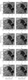 |
Fig. 7. Top row: comparison of the monochromatic image at the core of the Fe I 6173 Å spectral line for MOMFBD (left), equivalently ID in our notation, and the output of the recurrent network after all the 12 frames are considered (right), equivalently, |
4.2. Polarimetric demodulation
As mentioned in Sect. 3.1, the training and validation sets contain modulated Stokes parameters. Given that the linear and circular polarization signals in the Sun are often very small (normally much smaller than a percent in units of the continuum intensity except in strongly magnetized regions), any deconvolution process might run the risk of creating artificial signals. The reason is that polarimetric signals are obtained after combining several (typically four) observed frames. If during the deconvolution we introduce differential corrections in these frames, spurious signals will be created on the demodulation. To check for this issue, in Fig. 8 we display the demodulated circular polarization signals in the wing of the Fe I 6302 Å line. Likewise, Fig. 9 shows the demodulated Stokes V signals in the wing of the Ca II 8542 Å line. A direct comparison of the four magnetograms in Fig. 8 shows that the same fine structure is present in all of them, without any visible spurious signal appearing in any of the two neural architectures. It is obvious that the fine structure of the monochromatic image and the magnetogram are nicely recovered by our neural network approach, concentrating the polarization signals that were smoothed out by the atmosphere.
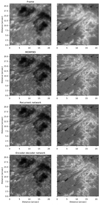 |
Fig. 8. Left panels: monochromatic images in the core of the Fe I 6302 Å line. Right panels: demodulated circular polarization signals for a single short-exposure frame, MOMFBD, and the two architectures we propose in this work. |
There are some differences, though, in the weaker signals of the Ca II 8542 Å line. The recurrent network seems to produce slightly better results than the encoder-decoder architecture. The clearly visible spatially correlated noise in the MOMFBD reconstruction is strongly dampened by the neural network approach, producing much cleaner magnetograms. Also, the spurious (at least not present in MOMFBD) structures that appear more conspicuously in the region around (20′,2.5′), which are especially visible in the encoder-decoder network, are not recovered by the recurrent architecture. These elongated structures seem to be a consequence of an artificial cross-talk between Stokes I and V produced by differential corrections in the different frames used by the polarimetric demodulation. A possible solution to these artifacts is proposed in Sect. 4.4. An issue, which according to our experiments apparently only happens in the encoder-decoder architecture, is that the contrast of the umbrae is reduced with respect to the surroundings.
It is also interesting to check the effect of the deconvolution on the Stokes profiles of an individual pixel. To this end, we display in Fig. 10 the Stokes profiles of a single pixel in both spectral lines. As reference, we show the Stokes profile of one of the frames of the burst in blue. We point out that the monochromatic deconvolution carried out by MOMFBD and the neural architectures proposed in this work do not produce any sizable artifact in these pixels with strong polarimetric signals. Pixels with weaker signal are, however, more affected by noise.
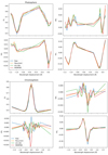 |
Fig. 10. Four Stokes profiles for the same individual pixel both in the photosphere and chromosphere. We compare the original raw frame, together with the profile obtained after deconvolving with MOMFBD and the two architectures proposed in this work. |
4.3. Hα monochromatic images
A neural network that is correctly trained should be generalizable to other inputs, providing reliable outputs. To this end, we tested the two networks developed in this work on images in the core of the Hα line. The core of the line displays very dynamic fibrilar structures that are believed to trace chromospheric material (Rutten et al. 2008), although its physics is still not fully understood (Leenaarts et al. 2015; Rutten & Rouppe van der Voort 2017). Some of the fibrils present in monochromatic Hα images are also partially seen in the core of the Ca II 8542 Å line, so one should expect the neural networks to generalize well. We use data obtained on 19 September 2016 from 09:30 to 10:00 with CRISP on the SST. The rows of Fig. 11 show two consecutive frames in the core of Hα, with one of the original frames in the first column and the deconvolved image using the encoder-decoder architecture in the second column. We do not display the results of the recurrent architecture to maximize the size of the images for a better comparison. The results are indeed very similar for the two neural networks. It is clear from these results that the network has been able to learn the process of image deconvolution, revealed by the huge amount of small-scale substructure that appears in the Hα filaments7.
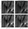 |
Fig. 11. Individual raw frames (left column) and deconvolved images (right column) for two different time steps of monochromatic images in the core of the Hα line. |
4.4. Frame shuffling and committees
All the experiments carried our so far use the input frames in the order obtained in the telescope. Changing the order of the input by reshuffling can be understood as another check for overtraining to verify that the networks have not memorized the ordering imposed during training. Additionally, the different outputs can be later combined following the neural network committee machine paradigm to improve the output. Given the nonlinear denoising character of the network, it makes sense to combine the outputs to improve the signal-to-noise ratio and reduce artifacts. This is indeed what happens, according to Fig. 12, with the encoder-decoder network (the same happens in the recurrent architecture). The fundamental reason for this behavior in the encoder-decoder architecture is that the first convolutional block, C0, 1, produces images with 64 channels by combining with different weights the seven input frames. This information is then propagated to the output and, as a consequence, a shuffling in the input layer produces a different output. A similar explanation is the source of the variability in the recurrent network. The first three rows of the figure display three different outputs by shuffling the input images in the core of the Ca II 8542 Å line in the left column and in the peak of Stokes V in the right column. It is clear that different shufflings produce different artifacts, especially in the lower right part of the image. This demonstrates that they are indeed produced by non-perfect reconstructions, which produce artificial polarization signals after demodulation. The last row gives the simplest committee machine one can think of, by plain averaging 20 such shufflings. More elaborate committees can be studied in the future. The spatial resolution of the final averaged image is practically the same as that of Fig. 9 because the real signals all appear at practically the same position and scale in all instances of the committee. However, the artifacts are different in all instances and tend to average to zero. Of special relevance is the disappearance of the fibrilar structures in the lower right corner on the circular polarization maps. Additionally, we witness a small decrease in the noise variance (around a factor of two), probably a mixture of artifact reduction plus a more efficient denoising.
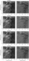 |
Fig. 12. Deconvolved images in the core of the Ca II 8542 Å line (left column) and demodulated circular polarization (right column) for different shuffling of the input using the encoder-decoder network. The final row shows the average of 20 different shufflings. |
5. Conclusions
We propose in this paper an end-to-end approach for multiframe blind deconvolution of solar images based on deep convolutional neural networks. We have used two different architectures. The first is a relatively simple encoder-decoder network, which needs to fix a-priori the number of frames considered. The second is a recurrent architecture that can work with an arbitrary number of frames. Both architectures are trained with data from CRISP and provide very fast image reconstructions.
We have demonstrated that the neural networks generalize well to unseen data. They are also able to keep the photometric quality of the data without compromising the modulated signals, thus providing polarimetry data of high quality. Additionally, the networks produce comparable results to the MOMFBD reconstruction without making use of simultaneous WB images. The only information needed for our end-to-end solution is the monochromatic frames produced by the etalon narrow filter.
Both networks are made available to the community, with all the training and testing details necessary for the reproduction of the results presented in this paper. The networks are developed with PyTorch, which makes very efficient use of any available GPU. Although the image correction is still not done in real time with current hardware for large images of 1k × 1k, we expect that future improvements in hardware and neural networks architectures that one can achieve after some ablation studies will allow this approach to deal with images in real time. In any case, the networks can be easily deployed on the telescope and produce quasi-real-time image reconstruction. Even if our approach is not used as the final processing for the science-ready data or managed to run in real time, it will produce very valuable information that can be used by the observer to see how science data will look like at the end of the MOMFBD processing.
Despite the successful neural networks presented here, we anticipate that improvements in the quality of the reconstruction can be achieved. First, one can use more elaborate loss functions. It is known that the ℓ2 norm of the residual tends to produce fuzzy reconstructions, especially when the number of frames is small. One can achieve better results by utilizing adversarial training (e.g., Ledig et al. 2016). Second, every burst of images is processed in isolation, so there is no transfer of information from burst to burst. Imposing some kind of time consistency can help the neural networks successfully correct bursts in which the seeing get worse. One can anticipate that a hierarchical architecture in which information is propagated for consecutive frames and also for consecutive bursts (similar to our recurrent architecture but with another level of hierarchy) might be worth trying. Finally, we note that training DNNs for multiframe image deconvolution can potentially be done using synthetic data. To this end, one could generate synthetic images from available magnetohydrodynamic simulations of the solar atmosphere and perturb them using artificial wavefronts from a synthetic turbulent atmosphere. The advantage in the synthetic case is that the unperturbed image is available to us, and the application of the MOMFBD algorithm is not needed. This can help to reduce some of the artifacts produced by the almost unavoidable presence of spatially correlated noise in the MOMFBD data. However, this approach might suffer from some lack of realism and it is not yet clear whether this approach will generalize correctly. It is currently very difficult to carry out simulations with a sufficiently realistic chromosphere. Therefore, the synthetic spectral lines are still not as realistic as desired. Moreover, computing the effect of a sufficiently realistic turbulent atmosphere is a hard task. One needs to take into account the known temporal correlation in the wavefront deformation and the presence of multiple anisoplanatic patches covered by the images. Work along these line is presumably needed in the future.
See, e.g., the curation on https://bit.ly/2ll0dQI
Gradients used during training become exponentially small when the neural network is sufficiently deep (e.g., https://en.wikipedia.org/wiki/Vanishing_gradient_problem).
As an example, applying one 3 × 3 kernel on an image produces a receptive field of size 3 × 3. Applying it twice increases the receptive field to a patch of size 5 × 5. On the contrary, if the image is halved in size between both convolutions, the receptive field increases to 7 × 7.
The code for the networks using PyTorch can be downloaded from https://github.com/aasensio/learned_mfbd
Training with stochastic gradient descent algorithms consists of iterating over the training set in batches. After each batch has been considered, the model parameters are updated with the “noisy” estimation of the gradient. An epoch is an iteration over the whole training set.
A movie showing the time evolution of Hα monochromatic images can be found on the repository for the code.
Acknowledgments
We thank Michiel van Noort for useful suggestions and the referee for many interesting suggestions that improved the paper. Financial support by the Spanish Ministry of Economy and Competitiveness through projects AYA2014-60476-P. We also thank the NVIDIA Corporation for the donation of the Titan X GPU used in this research. This research has made use of NASA’s Astrophysics Data System Bibliographic Services. JdlCR is supported by grants from the Swedish Research Council (2015-03994), the Swedish National Space Board (128/15), and the Swedish Civil Contingencies Agency (MSB). This project has received funding from the European Research Council (ERC) under the European Union’s Horizon 2020 research and innovation program (SUNMAG, grant agreement 759548). APY is supported by the German Government through DFG project “STOK3D Three dimensional Stokes Inversion with magneto-hydrostationary constraints”. The Swedish 1-m Solar Telescope is operated on the island of La Palma by the Institute for Solar Physics of Stockholm University in the Spanish Observatorio del Roque de los Muchachos of the Instituto de Astrofísica de Canarias. The Institute for Solar Physics is supported by a grant for research infrastructures of national importance from the Swedish Research Council (registration number 2017-00625). This study has been discussed in the workshop Studying magnetic-field-regulated heating in the solar chromosphere (team 399) at the International Space Science Institute (ISSI) in Switzerland. We acknowledge the community effort devoted to the development of the following open-source packages that were used in this work: numpy (numpy.org), matplotlib (matplotlib.org), and PyTorch (pytorch.org).
References
- Asensio Ramos, A., Requerey, I. S., & Vitas, N. 2017, A&A, 604, A11 [NASA ADS] [CrossRef] [EDP Sciences] [Google Scholar]
- Casini, R., de Wijn, A. G., & Judge, P. G. 2012, ApJ, 757, 45 [NASA ADS] [CrossRef] [Google Scholar]
- de la Cruz Rodríguez, J., Löfdahl, M.G., Sütterlin, P., Hillberg, T., & Rouppe van der Voort, L. 2015, A&A, 573, A40 [NASA ADS] [CrossRef] [EDP Sciences] [Google Scholar]
- Díaz Baso, C. J., & Asensio Ramos, A. 2018, A&A, 614, A5 [NASA ADS] [CrossRef] [EDP Sciences] [Google Scholar]
- He, K., Zhang, X., Ren, S., & Sun, J. 2016, IEEE Conference on Computer Vision and Pattern Recognition CVPR 2016, 770 [Google Scholar]
- Huertas-Company, M., Gravet, R., Cabrera-Vives, G., et al. 2015, ApJS, 221, 8 [NASA ADS] [CrossRef] [Google Scholar]
- Ioffe, S., & Szegedy, C. 2015, Proceedings of the 32Nd International Conference on International Conference on Machine Learning, ICML’15 , 37, 448 [Google Scholar]
- Kingma, D.P., & Ba, J. 2014, CoRR, [abs/1412.6980] [Google Scholar]
- Labeyrie, A. 1970, A&A, 6, 85 [Google Scholar]
- Ledig, C., Theis, L., Huszar, F., et al. 2016, CoRR, [abs/1609.04802] [Google Scholar]
- Leenaarts, J., Carlsson, M., & Rouppe van der Voort, L. 2015, ApJ, 802, 136 [Google Scholar]
- Löfdahl, M. G. 2002, in Image Reconstruction from Incomplete Data, eds. P. J. Bones,M. A. Fiddy, & R. P. Millane, 4792, 146 [NASA ADS] [CrossRef] [Google Scholar]
- Löfdahl, M. G., & Scharmer, G. B. 1994, A&AS, 107, 243 [NASA ADS] [Google Scholar]
- Löfdahl, M. G., Berger, T. E., Shine, R. S., & Title, A. M. 1998, ApJ, 495, 965 [NASA ADS] [CrossRef] [Google Scholar]
- Martínez Pillet, V., Del Toro Iniesta, J. C., Álvarez-Herrero, A., et al. 2011, Sol. Phys., 268, 57 [NASA ADS] [CrossRef] [Google Scholar]
- Nair, V., & Hinton, G. E. 2010, Proceedings of the 27th International Conference on Machine Learning (ICML-10), June 21–24, 2010 Haifa, Israel, 807 [Google Scholar]
- Paxman, R. G., Schulz, T. J., & Fienup, J. R. 1992, J. Opt. Soc. Am. A, 9, 1072 [NASA ADS] [CrossRef] [Google Scholar]
- Pesnell, W. D., Thompson, B. J., & Chamberlin, P. C. 2012, Sol. Phys., 275, 3 [NASA ADS] [CrossRef] [Google Scholar]
- Rutten, R. J. 2008, in First Results From Hinode, eds. S. A. Matthews,J. M. Davis, & L. K. Harra, ASP Conf. Ser., 397, 54 [NASA ADS] [Google Scholar]
- Rutten, R. J., & Rouppe van der Voort, L.H.M. 2017, A&A, 597, A138 [NASA ADS] [CrossRef] [EDP Sciences] [Google Scholar]
- Schawinski, K., Zhang, C., Zhang, H., Fowler, L., & Santhanam, G. K. 2017, MNRAS, 467, L110 [NASA ADS] [Google Scholar]
- Scherrer, P. H., Schou, J., Bush, R. I., et al. 2012, Sol. Phys., 275, 207 [Google Scholar]
- Schmidt, D., Gorceix, N., Goode, P. R., et al. 2017, A&A, 597, L8 [NASA ADS] [CrossRef] [EDP Sciences] [Google Scholar]
- Solanki, S. K., Barthol, P., Danilovic, S., et al. 2010, ApJ, 723, L127 [NASA ADS] [CrossRef] [Google Scholar]
- Suematsu, Y., Tsuneta, S., Ichimoto, K., et al. 2008, Sol. Phys., 249, 197 [NASA ADS] [CrossRef] [Google Scholar]
- van Noort, M., Rouppe van der Voort, L., & Löfdahl, M. G. 2005, Sol. Phys., 228, 191 [NASA ADS] [CrossRef] [Google Scholar]
- von der Lühe, O. 1993, A&A, 268, 374 [NASA ADS] [Google Scholar]
- Wieschollek, P., Hirsch, M., Schölkopf, B., & Lensch, H. 2017, IEEE International Conference on Computer Vision (ICCV 2017), 231 [CrossRef] [Google Scholar]
All Tables
All Figures
 |
Fig. 1. Architecture of the encoder-decoder deconvolution neural network. The network is composed of the input and eight super-blocks, each one made of a different number of blocks. The meanings of colors for the blocks are described in Sect. 2.1. The specific details for each block is described in Table 1. The numbers above the blocks label the super-blocks. |
| In the text | |
 |
Fig. 2. Upper panel: end-to-end deconvolution process, where the gray blocks are the deconvolution blocks described in the lower panel. Lower panel: internal architecture of each deconvolution block. Colors for the blocks are described in Sect. 2.2, with the specific details for each block being described in Table 2. |
| In the text | |
 |
Fig. 3. Selection of patches from the training set. First column: target MOMFBD corrected patch. Second column: output to the encoder-decoder network when converged. Third column: average of the seven frames of the burst, while the last two columns are two of these individual frames. |
| In the text | |
 |
Fig. 4. First column: images reconstructed with MOMFBD. Central column: output of the recurrent network. Right column: results for the encoder-decoder network. Upper row: image in the continuum around 6302 Å. Lower panel: image in the core of the line in a different part of the FOV. |
| In the text | |
 |
Fig. 5. Same as Fig. 4 but for the 8542 Å line. |
| In the text | |
 |
Fig. 6. Top panels: single raw image from the burst. Middle panels: reconstructed frames with the recurrent network. Lower panels: azimuthally averaged Fourier power spectra of the images. Left column: results from the continuum image at 6302 Å. Right column: results at the core of the 8542 Å line. All power spectra have been normalized to the value at the largest period (but not shown in the plot because it is outside the displayed range). |
| In the text | |
 |
Fig. 7. Top row: comparison of the monochromatic image at the core of the Fe I 6173 Å spectral line for MOMFBD (left), equivalently ID in our notation, and the output of the recurrent network after all the 12 frames are considered (right), equivalently, |
| In the text | |
 |
Fig. 8. Left panels: monochromatic images in the core of the Fe I 6302 Å line. Right panels: demodulated circular polarization signals for a single short-exposure frame, MOMFBD, and the two architectures we propose in this work. |
| In the text | |
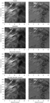 |
Fig. 9. Same as Fig. 8 but for the Ca II 8542 Å line. |
| In the text | |
 |
Fig. 10. Four Stokes profiles for the same individual pixel both in the photosphere and chromosphere. We compare the original raw frame, together with the profile obtained after deconvolving with MOMFBD and the two architectures proposed in this work. |
| In the text | |
 |
Fig. 11. Individual raw frames (left column) and deconvolved images (right column) for two different time steps of monochromatic images in the core of the Hα line. |
| In the text | |
 |
Fig. 12. Deconvolved images in the core of the Ca II 8542 Å line (left column) and demodulated circular polarization (right column) for different shuffling of the input using the encoder-decoder network. The final row shows the average of 20 different shufflings. |
| In the text | |
Current usage metrics show cumulative count of Article Views (full-text article views including HTML views, PDF and ePub downloads, according to the available data) and Abstracts Views on Vision4Press platform.
Data correspond to usage on the plateform after 2015. The current usage metrics is available 48-96 hours after online publication and is updated daily on week days.
Initial download of the metrics may take a while.


