| Issue |
A&A
Volume 688, August 2024
|
|
|---|---|---|
| Article Number | A88 | |
| Number of page(s) | 15 | |
| Section | Numerical methods and codes | |
| DOI | https://doi.org/10.1051/0004-6361/202449568 | |
| Published online | 08 August 2024 | |
Solar multiobject multiframe blind deconvolution with a spatially variant convolution neural emulator
1
Instituto de Astrofísica de Canarias (IAC), Avda Vía Láctea S/N,
38200
La Laguna, Tenerife,
Spain
e-mail: This email address is being protected from spambots. You need JavaScript enabled to view it.
2
Departamento de Astrofísica, Universidad de La Laguna,
38205
La Laguna, Tenerife,
Spain
e-mail: This email address is being protected from spambots. You need JavaScript enabled to view it.
Received:
10
February
2024
Accepted:
15
May
2024
Abstract
Context. The study of astronomical phenomena through ground-based observations is always challenged by the distorting effects of Earth’s atmosphere. Traditional methods of post facto image correction, essential for correcting these distortions, often rely on simplifying assumptions that limit their effectiveness, particularly in the presence of spatially variant atmospheric turbulence. Such cases are often solved by partitioning the field of view into small patches, deconvolving each patch independently, and merging all patches together. This approach is often inefficient and can produce artifacts.
Aims. Recent advancements in computational techniques and the advent of deep learning offer new pathways to address these limitations. This paper introduces a novel framework leveraging a deep neural network to emulate spatially variant convolutions, offering a breakthrough in the efficiency and accuracy of astronomical image deconvolution.
Methods. By training on a dataset of images convolved with spatially invariant point spread functions and validating its generalizability to spatially variant conditions, this approach presents a significant advancement over traditional methods. The convolution emulator is used as a forward model in a multiobject multiframe blind deconvolution algorithm for solar images.
Results. The emulator enables the deconvolution of solar observations across large fields of view without resorting to patch-wise mosaicking, thus avoiding the artifacts associated with such techniques. This method represents a significant computational advantage, reducing processing times by orders of magnitude.
Key words: methods: data analysis / methods: numerical / techniques: image processing / Sun: atmosphere
© The Authors 2024
 Open Access article, published by EDP Sciences, under the terms of the Creative Commons Attribution License (https://creativecommons.org/licenses/by/4.0), which permits unrestricted use, distribution, and reproduction in any medium, provided the original work is properly cited.
This article is published in open access under the Subscribe to Open model. This email address is being protected from spambots. You need JavaScript enabled to view it. to support open access publication.
1 Introduction
Ground-based observations are always affected by the perturbations produced by the atmosphere. The turbulence induced by unavoidable air motions (seeing) produces changes in the refraction index at many spatial and temporal scales. These changes affect the incoming light from astronomical objects by producing local deviations. The phase of the incoming wavefront, which can be safely assumed to be flat outside the Earth’s atmosphere, is corrugated by the presence of atmospheric turbulence. This produces, in general, a blurring effect that is absent in observations from observatories located in space.
The temporal and spatial characteristics of the turbulence change with time and they are difficult to predict. The temporal correlation time of the atmosphere is typically very short, close to milliseconds. As a consequence, observations with long integration times (longer than the correlation time) average the state of the atmosphere over many realizations. In such cases, because of the ensuing information loss, the blurring effect of the atmosphere is unavoidable and cannot be corrected for. On the other hand, observations with very short integration times (of the order of the correlation time) freeze the state of the atmosphere and can be used to reconstruct the original object from the information present in the speckle distribution. Short integration times are nevertheless affected by noise and many such observations are required to reduce its impact on the final result. This is especially relevant in low-luminosity observations (e.g., observing exoplanets, faint stars, etc.) or when carrying out high-spectral-resolution spectropolarimetry. Regarding the spatial correlation, strong turbulence produces very small eddies (of the order of centimetres). As a consequence, the ensuing wavefront is very corrugated by the presence of many short-scale eddies covering the projection of the pupil of the telescope on the sky. This is especially relevant for large-aperture telescopes, where the size of the pupil is large. To make things more challenging, the turbulence existing at different heights in the atmosphere is potentially different. Turbulence close to the pupil of the telescope (low-height turbulence) produces the same blurring across the entire field of view (FoV). Meanwhile, turbulence at higher altitudes produces differential blurring in different parts of the FoV, known as anisoplanatism.
Several techniques have been developed for reducing the perturbing effect of the atmosphere. Adaptive optics (AO) is arguably one of the most successful, and is based on the measurement of the instantaneous wavefront (ideally at millisecond cadence) and compensation for the measured phase using active optics, such as deformable mirrors. Ground layer AO, which measure the wavefront in the pupil of the telescope and correct for it using deformable mirrors, produce an improvement of the image quality over the whole FoV. However, the presence of turbulence at high atmospheric layers, which produces differential effects in different parts of the FoV, requires the application of multiconjugate AO systems. These systems are in charge of measuring the turbulence at many atmospheric layers in real time and correcting for them using deformable mirrors conjugated at different heights in the atmosphere. These systems are still in their infancy and operating them in real time is very complex.
Another highly successful technique for reducing the effect of the atmosphere is post facto image reconstruction. These methods are based on using a physical model for the formation of an image under a turbulent atmosphere and inferring the object and the instantaneous status of the atmosphere by applying a maximum likelihood (ML) approach. This requires the observation of several short-exposure-time observations. Better results are obtained when using a relatively large number of observations (of the order of tens for typical solar observations). The problem to be solved is of the blind deconvolution kind, because neither the object nor the instantaneous wavefront is known and both need to be inferred simultaneously. Like any blind deconvolution, the problem is severely ill-defined and some type of regularization is required. In the literature, one can find methods based on maximum a posteriori, which make use of Bayes’ theorem and explicit priors both for the object and the wavefronts (see Molina et al. 2001, and references therein). Other methods use the simpler ML approach but introduce regularization by using a low-complexity description of the wavefront and making use of spatial filtering to avoid the appearance of unphysically high frequencies in the deconvolved image (Löfdahl & Scharmer 1994; van Noort et al. 2005).
The most widespread physical model used for blind deconvolution requires the assumption of a spatially invariant point spread function (PSF). Its main advantage is that the convolution of the object with the PSF can be computed very efficiently using the fast Fourier transform (FFT). As a consequence, the deconvolution can only be carried out inside one anisoplanatic patch, where this assumption holds. This assumption is somewhat restrictive under the presence of strong turbulence or when observing with a large-aperture telescope. In those two cases, the anisoplanatic patch becomes very small. Arguably the most widespread solution to overcome this limitation is the application of the overlap-add (OLA) method. This method requires mosaicking the image in sufficiently small overlapping patches, deconvolving each patch independently under the assumption of a spatially invariant PSF, and finally merging all patches together. This merging operation is commonly performed by averaging each patch with a weighting scheme to smoothly connect the overlapping borders. This approach has been very successful in solar observations, as demonstrated by the success of the multiframe multiobject blind deconvolution code (MOMFBD; van Noort et al. 2005). However, more elaborate and precise methods for dealing with spatially variant PSFs do exist, such as the widespread method of Nagy & O’Leary (1998) and the recent space-variant OLA (Hirsch et al. 2010). A good review of these techniques can be found in Denis et al. (2015).
Here, we propose a novel approach to deal with spatially variant PSFs. We propose the use of a deep neural network to emulate the spatially variant convolution with a PSF that can be arbitrarily different in all pixels in the FoV. We check that this spatially variant convolution emulator (SVCE), although trained with spatially invariant convolutions, correctly approximates a spatially variant convolution with good precision. The deep learning model is fully convolutional, meaning that it generalizes to images of arbitrary size. We demonstrate the use of this SVCE as a very efficient forward model to carry out multiobject multiframe blind deconvolutions in large FoVs without using any mosaicking.
2 Neural spatially variant convolution
In the general case in which the PSF of an optical system (the atmosphere plus the telescope and instruments in our case) is spatially variant, the intensity I(r) received at a certain pixel location defined by the coordinates r = (x, y) is given by the following integral in the auxiliary variable r′:
![Mathematical equation: $\[I(\mathbf{r})=\int O\left(\mathbf{r}^{\prime}\right) S\left(\mathbf{r}, \mathbf{r}^{\prime}\right) \mathrm{d} \mathbf{r}^{\prime},\]$](/articles/aa/full_html/2024/08/aa49568-24/aa49568-24-eq1.png) (1)
where O(r′) is the object intensity before the optical system and S(r, r′) is the local PSF at point r. Computing the measured intensity for a pixellized image of size N × N requires the computation of N2 such integrals. Therefore, the computation of the final image scales as
(1)
where O(r′) is the object intensity before the optical system and S(r, r′) is the local PSF at point r. Computing the measured intensity for a pixellized image of size N × N requires the computation of N2 such integrals. Therefore, the computation of the final image scales as ![Mathematical equation: $\[\boldsymbol{\mathcal{O}}\]$](/articles/aa/full_html/2024/08/aa49568-24/aa49568-24-eq2.png) (N4), which is prohibitive for large images. One way of reducing the computing time is by assuming a relatively compact PSF, so that it can be correctly defined in a pixellized image of size M × M, with M ≪ N. In such case, the computing work scales as
(N4), which is prohibitive for large images. One way of reducing the computing time is by assuming a relatively compact PSF, so that it can be correctly defined in a pixellized image of size M × M, with M ≪ N. In such case, the computing work scales as ![Mathematical equation: $\[\boldsymbol{\mathcal{O}}\]$](/articles/aa/full_html/2024/08/aa49568-24/aa49568-24-eq3.png) (N2 M2), which can still be prohibitive for large images.
(N2 M2), which can still be prohibitive for large images.
Contrarily, when the PSF is spatially invariant, S(r, r′) = S(r − r′) is fulfilled, and the integral can be computed by using the convolution theorem:
![Mathematical equation: $\[I(\mathbf{r})=O(\mathbf{r}) \otimes S(\mathbf{r}).\]$](/articles/aa/full_html/2024/08/aa49568-24/aa49568-24-eq4.png) (2)
(2)
From a computational point of view, the spatially invariant case can be very efficiently computed using the FFT, since the FFT of a 2D image can be computed in ![Mathematical equation: $\[\boldsymbol{\mathcal{O}}\]$](/articles/aa/full_html/2024/08/aa49568-24/aa49568-24-eq5.png) (N2 log N) operations. Three FFTs are required to compute the convolution, so that the total computing timescales as
(N2 log N) operations. Three FFTs are required to compute the convolution, so that the total computing timescales as ![Mathematical equation: $\[\boldsymbol{\mathcal{O}}\]$](/articles/aa/full_html/2024/08/aa49568-24/aa49568-24-eq6.png) (N2 log N).
(N2 log N).
2.1 Point spread function model
Given the enormous computational complexity of the spatially variant convolution, we propose the use of a neural network to emulate this process. To this end, we compute the PSF as the autocorrelation of the generalized pupil function P (e.g., van Noort et al. 2005), calculated here with the aid of the inverse Fourier transform ℱ−1:
![Mathematical equation: $\[S(\mathbf{r})=\left|\mathcal{F}^{-1}(P(\mathbf{v}))\right|^2.\]$](/articles/aa/full_html/2024/08/aa49568-24/aa49568-24-eq7.png) (3)
(3)
The generalized pupil function is given by the following general expression:
![Mathematical equation: $\[P(\mathbf{v})=A(\mathbf{v}) e^{i \varphi(\mathbf{v})},\]$](/articles/aa/full_html/2024/08/aa49568-24/aa49568-24-eq8.png) (4)
(4)
where A(v) represents the amplitude of the pupil (we assume it fixed and known), and takes into account the size of the primary mirror, the shadow of the secondary mirror or any existing spider, φ(v) is the phase of the wavefront, and v is the coordinate on the pupil plane. The imaginary unit number is denoted as i, as usual. We choose to parameterize the phase of the wavefronts φ(v) through suitable basis functions. This is a very efficient way of regularizing any blind deconvolution problem since PSFs are, by construction, sparsely parameterized and are also strictly positive. In this study we use the Karhunen-Loève (KL; Karhunen 1947; Loève 1955) basis (see also, van Noort et al. 2005). This basis is constructed as a rotation of the Zernike polynomials (Zernike 1934), with coefficients found by diagonalizing the covariance matrix of the Kolmogorov turbulence (see Roddier 1990). Therefore:
![Mathematical equation: $\[\varphi(\mathbf{v})=\sum_{l=1}^M \alpha_l \mathrm{KL}_l(\mathbf{v}),\]$](/articles/aa/full_html/2024/08/aa49568-24/aa49568-24-eq9.png) (5)
(5)
where M is the number of basis functions and αl is the coefficient associated with the basis function KLl.
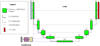 |
Fig. 1 U-Net deep neural network used in the present work as an emulator for the spatially variant convolution. M′ = M + 1 is the number of channels of the input tensor, which is built by concatenating the image of interest and the spatially variant images of the M Karhunen-Loève. All green blocks of the encoder are conditioned to the specific instrumental configuration as described in Sect. 2.2.1 via the encoding fully connected network shown in the figure. The gray box refers to the one-hot encoding of the instrumental configuration. |
2.2 The deep learning model
Our proposal for SVCE is to use a conditional U-Net (shown in graphical representation in Fig. 1), a variation of the very succesful U-Net model of Ronneberger et al. (2015) widely used in image-to-image problems. This model will produce a discretized image, i, the result of convolving the object intensity, o, with a spatially variant PSF characterized by per-pixel KL coefficients, α:
![Mathematical equation: $\[i=f(x=\{o, \alpha\}),\]$](/articles/aa/full_html/2024/08/aa49568-24/aa49568-24-eq10.png) (6)
(6)
where f is the deep neural model described in the following. When discretized, i and o are 4D tensor of size (B, 1, X, Y), where B is the batch size, X and Y are the spatial sizes of the image and 1 is the number of channels. Similarly, α is a 4D tensor of size (B, M, X, Y), where M is the number of KL coefficients. Both o and α are concatenated along the channel dimension to produce x, a 4D tensor of size (B, M + 1, X, Y), and used as input to the neural network. The graphical representation of Fig. 1 clearly shows two differentiated parts: an encoder that reduces the size of the images while increasing the number of channels and a decoder that does the opposite operation. Some information from the encoder is allowed to be passed to the decoder through skip connections, which greatly improves the performance of the model. For clarity, we detail the operations carried out in each layer in the following.
2.2.1 Encoder
The input tensor (i) is first passed through the following two sets of operations:
![Mathematical equation: $\[\begin{aligned}\hat{p}_1 & =\operatorname{ReLU}\left(\operatorname{BN}\left(\operatorname{Conv}_3(C, x)\right)\right) \\p_1 & =\operatorname{ReLU}\left(\operatorname{BN}\left(\operatorname{Conv}_3\left(C, \hat{p}_1\right)\right)\right),\end{aligned}\]$](/articles/aa/full_html/2024/08/aa49568-24/aa49568-24-eq11.png) (7)
(7)
where Conv3(C, x) is a 2D convolutional layer with C = 64 kernels (we did not explore other values of C) of size 3 × 3 (the size of the kernel is labeled with the subindex), followed by batch normalization (BN; Ioffe & Szegedy 2015) and a rectified linear unit activation (ReLU(x) = max(0, x)). The resulting tensor is then halved in size by using a 2 × 2 max-pooling operation. This interchange of spatial information into channel information in the low resolution features pj efficiently exploits spatial correlation. After every max-pooling, the resulting tensor is passed through the following two operations:
![Mathematical equation: $\[\begin{aligned}\hat{p}_{j+1} & =\operatorname{ReLU}\left(\operatorname{BN}\left(\operatorname{Conv}_3\left(2^{j+1} C, p_j\right)\right)\right), \\p_{j+1} & =\operatorname{ReLU}\left(\operatorname{BN}\left(\operatorname{Conv}_3\left(2^{j+1} C, \gamma \hat{p}_{j+1}+\beta\right)\right)\right),\end{aligned}\]$](/articles/aa/full_html/2024/08/aa49568-24/aa49568-24-eq12.png) (8)
(8)
where j = 1,..., 4. These expressions are similar to those of Eq. (7), but with two scalars γ and β that are used for conditioning the network on the specific instrument. The values of γ and β are shared for all layers in the encoder. This approach for conditioning is an extremely simplified version of the feature-wise linear modulation (FiLM; Perez et al. 2017), and the details are explained in the following paragraph. Additionally, the number of channels is doubled with respect to the previous level. The number of channels in the lowest resolution features is 24C = 1024, and the spatial resolution of the input has been decreased by a factor of 24 = 16. This constitutes the bottleneck of the U-Net model and turns out to be crucial for emulating very extended PSFs resulting from very deformed wavefronts.
We want this model to be as general as possible, so that it can be applied to telescopes of arbitrary diameter, any wavelength of choice and any pixel size in the camera. This would require that we condition the U-Net on a vector that encodes all this information. Training such model would require the generation of a suitable training set that covers all possible combinations. Since this is not realistic, and indeed is never the case in reality, we prefer to use a rather pragmatic approach for conditioning. Given that only a few combinations of telescopes, cameras and wavelength are used routinely, we label each combination with an index i = 1,..., I, where I is the total number of available combinations. We consider in this work the Swedish Solar Telescope (SST) with the CRisp Imaging Spectropolarimeter (CRISP; Scharmer et al. 2008) and the CHROMospheric Imaging Spectrometer (CHROMIS; Scharmer 2017), together with the GREGOR telescope with the High-resolution Fast Imager (HiFI; Denker et al. 2023). The model can be easily extended to other telescopes and instruments. We transform each index into a one-hot vector1 of length I. These one-hot encodings are then passed through a small fully connected network (FCN) (displayed in pink in Fig. 1) with 2 hidden layers and 64 neurons in each layer. The output of this FCN produces the two scalars γ and β. We have not explored more complex conditioning schemes (e.g., vector conditioning instead of scalar), but we argue that this simple global approach is sufficient for our purposes, at least from what emerges from our results.
Considered instrumental configurations.
2.2.2 Decoder
In the decoder part of the U-Net, the features are doubled in size again by using linear upsampling until reaching the original size. Skip connections propagating information from the encoder at each scale are added for the efficient propagation of gradients to all layers. This greatly accelerates the performance and training time of the U-Net model. After each upsampling and concatenation with the features of the same scale coming from the encoder, the following operations are carried out:
![Mathematical equation: $\[\begin{aligned}& \hat{p}_{j+1}=\operatorname{ReLU}\left(\operatorname{BN}\left(\operatorname{Conv}_3\left(2^{j+1} C, p_j\right)\right)\right), \\& p_{j+1}=\operatorname{ReLU}\left(\operatorname{BN}\left(\operatorname{Conv}_3\left(2^{j+1} C, \hat{p}_{j+1}\right)\right)\right),\end{aligned}\]$](/articles/aa/full_html/2024/08/aa49568-24/aa49568-24-eq13.png) (9)
(9)
where j = 4,..., 1. We note that we do not condition the decoder on the specific instrument configuration. We found it unnecessary but it can be seamlessly added if needed. A final 1 × 1 convolutional layer produces the output y:
![Mathematical equation: $\[y=\operatorname{Conv}_1\left(1, p_{j+1}\right),\]$](/articles/aa/full_html/2024/08/aa49568-24/aa49568-24-eq14.png) (10)
(10)
Our specific model is fully convolutional, so that the output and input spatial sizes are the same if the input tensor spatial sizes are multiple of 24. Otherwise, the input and output can differ in a few pixels. The total number of trainable parameters of the neural model is 17.3M.
2.3 Training
The training of the model is inspired by the approach followed by Cornillère et al. (2019). The idea is to use a suitable set of images with sufficient spatial variability and convolve them with spatially invariant PSFs. Despite being trained with spatially invariant PSFs, the fact that we supply the KL coefficients with spatial structure produces a model that is able to learn spatially variant convolutions, as we demonstrate in Sec. 2.4.
Although the current status of solar magneto hydrodynamic simulations is very advanced, especially for generating solar-like images, there are not enough simulations of quiet and active regions that are available for the community for a proper training. In an effort to overcome this difficulty, we decided to check whether the U-Net can be trained with images not specifically coming from solar structures. From a conceptual point of view, the effect of a spatially variant convolution should be independent of the specific object. We decided to use publicly available repositories of images. One obvious possibility is ImageNet (Deng et al. 2009), which contains almost 15M high-resolution images, each one classified in a set of 1000 classes. We discarded this option since the amount and sizes of the images is huge and makes downloading and training the model very computationally demanding. A better option for our purposes is Stable ImageNet-1K2, a set of 512 × 512 pixel images artificially generated with the Stable Diffusion 1.4 generative model (Rombach et al. 2022). The database contains 100 images for each one of the 1000 classes of ImageNet. All images are resized to 152 × 152 pixels for training.
The PSFs are obtained from the wavefront coefficients using Eqs. (3)–(5). The α coefficients are randomly sampled using the approach of Roddier (1990). The PSF depends on the telescope diameter D, central obscuration D2, pixel size and wavelength. All considered combinations are shown in Table 1. We consider random wavefronts with turbulence characterized by a Fried radius (r0) in the range 3-15 cm. The variance of the KL modes are proportional to (D/r0)5/3, so that smaller Fried radii lead to more deformed wavefronts, which produce more complex and extended PSFs. Every image from Stable ImageNet-1K is then convolved with the computed PSF using the FFT, thanks to the assumption of a spatially invariant PSF. Given that the images are nonperiodic, we utilize a Hanning window with a transition of 12 pixels in each border to apodize them so that artifacts are avoided when using the FFT. Convolved images are then cropped to 128 × 128 to remove the apodized region. With this approach, 90k such images are used for training and 10k for validation. To increase the variability, we include additional augmentations by randomly rotating (0°, 90°, 180° and 270°) and flipping horizontally and vertically the images. In our initial experiments using only images from Stable ImageNet-1K, we realized that the model was not properly learning the specific shape of the PSF, although the output of the model was very similar to the target. For this reason, and to force the model to properly learn the shape of the PSF, we substituted 20% of the images of the training set by fields of randomly located point-like objects in a black background. The convolution of these images with a PSF gives the shape of the PSF repeated several times in the image. After adding them to the training set, we checked that this helped a lot in recovering a much better shape of the PSF, as shown below.
The training proceeds by using the output of the network, y and the target convolved image, t, and minimizing the following loss with respect to the weights of the U-Net and those of the conditioning network:
![Mathematical equation: $\[\mathcal{L}=\|y-t\|^2+\lambda_{\text {grad }}\|\nabla y-\nabla t\|^2+\lambda_{\text {flux }}\|\langle y\rangle-\langle t\rangle\|^2.\]$](/articles/aa/full_html/2024/08/aa49568-24/aa49568-24-eq15.png) (11)
(11)
The first term is proportional to the mean squared error, which forces the per-pixel output image to be as similar as possible to the target, measured with the ℓ2 norm. The second term forces the horizontal and vertical gradients to be as similar as possible. We realized that adding this term produced an improved quality for the convolutions, specially for the point-like objects. The gradients are implemented using Sobel operators. Finally, a third term forces the total flux of the image to be preserved. The hyperparameters λgrad = 10 and λflux = 1 produced good results. We leave for the future a sensitivity analysis to the hyperparameters, which will require lots of computing time.
We trained for 100 epochs, ending up with the model that gives the best validation loss. We used the Adam optimizer (Kingma & Ba 2014) with a learning rate that starts at 3 × 10⁻⁴ and is slowly decayed to 6 × 10⁻⁵ following a cosine rule (Loshchilov & Hutter 2017). The model is trained on a single NVIDIA GeForce RTX 2080 Ti GPU using half precision, to make a more efficient use of the video memory and tensor cores on board the GPU. The training is implemented and run using PyTorch 2.0.1 (Paszke et al. 2019).
Figure 2 shows the training and validation losses during training. The training proceeds nominally although the validation set clearly shows a saturation of the capabilities of the model around epoch 50. Along the training epochs, we find a rather variable validation loss, mainly produced by the strong penalization in the point-like objects when the proper PSF is not produced in the output. In any case, we only see some hints of overfitting at the very end of the training; to overcome this, we select the model producing the best validation loss as the optimal for our selection of hyperparameters.
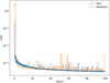 |
Fig. 2 Evolution of training and validation losses for all epochs. The neural network does not show overtraining, although a saturation occurs after epoch ~50. |
2.4 Validation
Figure 3 shows some examples of the behavior of the SVCE on the validation set. The upper row shows either the original unperturbed images from Stable ImageNet-1K or the synthetic point-like images. Some images appear rotated due to the augmentation process. The second and third rows show the target image and the output of the SVCE, respectively. Finally, the fourth row displays the scaled residual between the target and the output of the model. Since images are normalized to the interval [0, 1], the residual shows differences below 5%. The labels indicate the normalized mean squared error (NMSE), computed as:
![Mathematical equation: $\[\mathrm{NMSE}=\frac{\|y-t\|^2}{\|t\|^2}.\]$](/articles/aa/full_html/2024/08/aa49568-24/aa49568-24-eq16.png) (12)
(12)
Visually, both the target and the output of the model look very similar. Differences are, however, more conspicuous for the point-like images. Very complex PSFs with lots of speckles are difficuly to be reproduced. We argue that improved models can be obtained by carrying out a hyperparameters tuning phase as well as using solar synthetic images during the training. Improvements to the U-Net model can also produce better final convolved images. We are, though, happy with the trained SVCE given its proof-of-concept character, but work along the lines described above can decisively impact positively on the quality of the SVCE and the ensuing reconstructions.
Given that the neural model has been trained with synthetic images of the Stable ImageNet-1K database, it is important to test how it generalizes to other type of images. In particular, we need to test whether the method does a good job in typical solar images. To this end, we used a continuum image from a snapshot of the quiet Sun hydrodynamical simulation of Stein & Nordlund (2012) (see also Stein 2012). The pixel size of this snapshot is 0.066 arcsec, which is close enough to the pixel size of the CRISP instrument. Consequently, we used the CRISP8542 configuration for the SVCE. Figure 4 shows the ability of the model to produce spatially variant convolutions in a subfield of 256 × 256 pixels of the original snapshot. We demonstrate how the neural SVCE is able to mimick the effect of a defocus PSF that is gradually shifted along the diagonal of the image. To this end, we simply set the KL coefficient for defocus equal to a Gaussian centered on pixels along the diagonal with a standard deviation such that it affects several granules. The neural model is able to seamlessly reproduce this spatially variant convolution running the neural model in evaluation mode. Given the excellent parallelization capabilities of GPUs, if enough GPU memory is available, all images in Fig. 4 can be obtained in a single forward pass.
In order to test the reliability of the spatially variant convolution of the SVCE, we compared the results with the ones obtained using classical techniques (see Fig. 5). To this end, we compute the convolution of the original image with 2562 different PSFs, each one corresponding to the defocus found in every single pixel (i, j). The construction of the final image loops over all pixels in the output image, and the output is computed by multiplying the PSF associated with the pixel (centered on the pixel) and the original image. This can be interpreted as an OLA method with a 1-pixel mosaicking window. In our machine, the computation of the 2562 convolutions takes ~12 min in CPU, which is dominated by the computation of the PSF from the perpixel wavefront coefficients. The neural model takes ~100 ms in the same CPU, without any effort in optimization, which is a speed-up of ~3000 times. A large part of this gain is produced by not having to compute the PSF for every pixel from the wavefront coefficients. Benchmarks are displayed in Fig. 6, where the computing time per convolution is shown as a function of the size of the image and the batch size. The SVCE is able to process images several orders of magnitude faster than the classical method.
The comparison is shown in Fig. 5. Our SVCE is able to produce very similar results with a significant reduction in computing time. The neural SVCE does not require any apodization, so it works even at the borders of the image. For comparison, we show synthetic diffraction image for a telescope of 1 m, together with the original image from the simulation. The SVCE is able to reproduce the diffraction image away from the defocus point and a defocused image at the position of the defocus. The maximum absolute residual is of the order of 4% (images are normalized to 1), with a NMSE of 1.6 × 10⁻⁴.
The effect of the SVCE on point-like objects is displayed on Fig. 7. We show the approximate PSF obtained with the neural model, and it is compared with the correct PSF obtained from the KL modes. We show results for different realizations of Kolmogorov turbulence with different Fried radii. The neural model is able to nicely approximate the PSF for weak and medium turbulence, although its capabilities are degraded for very strong turbulence. This is demonstrated in Fig. 8, where the NMSE is shown to monotonically decrease for larger values of the Fried radius. This would require improvements on the training, as described above. Anyway, we argue that the general shape of the PSF is correctly recovered, which is enough for a good deconvolution of observations, especially when adaptive optics is used.
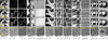 |
Fig. 3 Samples from the training set, showing the capabilities of our model. The upper row displays 12 original images from Stable ImageNet-1K and a synthetic image of point-like objects. The second row displays the target convolved image, with a PSF that is compatible with Kolmogorov turbulence. The third rows shows the output of our model, with the fourth row displaying the residuals. |
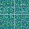 |
Fig. 4 Spatially variant convolution with a defocus obtained with the SVCE. The defocus PSF is shifted along the diagonal of the image. |
3 Multiobject multiframe spatially variant blind deconvolution
The trained neural SVCE can be used as a replacement of the computationally intensive forward model in multiframe blind deconvolution problems in cases in which the PSF is spatially variant. Since the SVCE can deal with per-pixel PSFs, one can get rid of the mosaicking process and convolve large images much faster. In this section we analyze its performance on standard optimization-based methods similar to the one proposed by Löfdahl & Scharmer (1994) and van Noort et al. (2005). We show that the SVCE produces a significant gain in computing time, allowing us to carry out image correction in a full FOV in one go. In a set of reduced experiments we show that it is possible to obtain reconstructions of good quality, almost comparable to those obtained with the version of the MOMFBD code that we used (Löfdahl et al. 2021).
3.1 Formulation of the problem
Following the standard procedure, let us consider that we simultaneously observe K objects (e.g., monochromatic images of the same region of the Sun at two different wavelenghts) and collect L short exposure frames with a ground-based instrument of a stationary object outside Earth’s atmosphere. All objects at the same frame are assumed to be affected by exactly the same wavefront. In our case, given our scientific interests, our object is a small region on the surface of the Sun, but the results can be applied to any other point-like or extended object. We note, in passing, that if this method is to be applied to point-like objects, better results would be obtained by training the neural SVCE only with point-like objects.
The exposure time of each individual frame is short enough – of the order of a few milliseconds – so that one can assume that the atmosphere is “frozen”, i.e., it does not evolve during the integration time. Additionally, we assume that the total duration of the burst is shorter than the solar evolution timescales, so that the object can be safely assumed to be the same for all frames. Let us represent the observed image of object k at frame l as ikl. As a consequence, using the neural SVCE of Eq. (6), with its weights frozen, the observed image can be approximated as:
![Mathematical equation: $\[i_{k l}=f\left(\left\{o_k, \alpha_l\right\}\right)+n_{k l} \text {, }\]$](/articles/aa/full_html/2024/08/aa49568-24/aa49568-24-eq17.png) (13)
(13)
where αl are the per-pixel wavefront coefficients (44 in our case because the SVCE was trained with that number of modes) for frame l ∈ {1 ... L} and nkl represents the noise term. The SVCE is, consequently, used as a substitute of the forward problem, which would consist of mosaicking, convolving with per-patch PSFs and merging the patches together. We note that, since all objects observed simultaneously share the same atmospheric perturbations, the PSF simply changes because of the potential wavelength difference between the objects.
The spatially variant multiobject multiframe blind deconvolution problem (SV-MOMFBD) consists of inferring the true objects ok and the wavefront coefficients αl from the observed images ikl using the SVCE as a forward model. This is accomplished by maximizing the likelihood of the observed images. Under the assumption of Gaussian noise, the maximum-likelihood solution can be obtained by minimizing the following loss function:
![Mathematical equation: $\[L(o, \boldsymbol{\alpha})=\sum_{k, l, x, y} \gamma_{k l} \| i_{k l}-f\left(\left\{o_k, \alpha_l\right\} \|^2\right.,\]$](/articles/aa/full_html/2024/08/aa49568-24/aa49568-24-eq18.png) (14)
(14)
where the norms are calculated over all pixels for all frames and objects. The weights γkl are often set inversely proportional to the noise variance. For simplicity, we decided to select γkl = 1 for all k and l. The assumption of Gaussian statistics is approximately valid in the solar case, in which the number of photons is large and the dynamic range of the illumination is small. If this is not the case but the number of photons is still large, one should take into account that the noise variance is proportional to the mean expected number of photons in each pixel. In low illumination cases, one should resort to Poisson statistics.
 |
Fig. 5 Original image from the Stein (2012) simulation (first panel) together with the image after diffraction when observed with SST/CRISP at 8542 Å (second panel). The third panel displays the spatially variant convolution with a region of defocus computed using per-pixel convolution, with the fourth panel showing the results obtained with the neural SVCE. The last panel displays the residuals, with an NMSE of 1.6 × 10⁻⁴. |
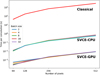 |
Fig. 6 Computing time per convolution as a function of the size of the image and the batch size for the SVCE, both in CPU and GPU. As a comparison, we show results obtained for the classical method of computing the convolution of the image with a PSF for every pixel. |
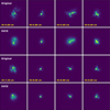 |
Fig. 7 Comparison of the exact PSFs obtained for a specific realization of a Kolmogorov atmosphere with different values of the Fried radius and the neural approximation. Although it captures the general behavior of the PSF, the behavior of the neural model is worse as the level of turbulence increases. Fig. 7. Comparison of the exact PSFs obtained for a specific realization of a Kolmogorov atmosphere with different values of the Fried radius and the neural approximation. Although it captures the general behavior of the PSF, the behavior of the neural model is worse as the level of turbulence increases. |
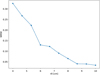 |
Fig. 8 Evolution of the NMSE as a function of the Fried radius, showing that the behavior of the neural model worsens when the level of turbulence increases. |
3.2 Regularization
Even if the number of observed frames is large, the maximum likelihood solution can lead to artifacts in the reconstruction. To minimize these effects, one can apply early stopping techniques or use additional regularization techniques. We consider two different regularization techniques. The first one is based on filtering the Fourier transform of the objects. In this case, we substitute the object in Eq. (14) by its filtered version:
![Mathematical equation: $\[o_k^*=\mathcal{F}^{-1}\left(H \cdot \mathcal{F}\left(o_k\right)\right),\]$](/articles/aa/full_html/2024/08/aa49568-24/aa49568-24-eq19.png) (15)
(15)
where H is a filter that removes the high frequencies of the object. This idea was proposed by Löfdahl & Scharmer (1994) using a relatively complex and ad hoc algorithm for computing H. Since that specific regularization cannot be easily applied to our case, we instead consider a simple Fourier filtering to reduce the presence of frequencies above the diffraction limit. In this case, we find good results with a flat-top filter with a smooth transition to zero close to the diffraction cutoff frequency. We build this filter as the convolution of a Gaussian and a rectangle, where ν is the spatial frequency in the Fourier plane in units of the cutoff frequency, w defines the width of the filter and n controls the smoothness of the transition:
![Mathematical equation: $\[H(k)=\frac{1}{2}\left\{\operatorname{erf}\left[n\left(\nu+\frac{w}{2}\right)\right]-\operatorname{erf}\left[n\left(\nu-\frac{w}{2}\right)\right]\right\}.\]$](/articles/aa/full_html/2024/08/aa49568-24/aa49568-24-eq20.png) (16)
(16)
Good filtering is found for w = 1.8 (slightly less than the diffraction) and n = 20.
We additionally explore Tikhonov regularization (i.e., ℓ2 regularization) for the spatial gradients of the objects and the wavefront coefficients. This encourages smooth solutions and helps reduce the artifacts. The final loss function is given by:
![Mathematical equation: $\[L(o, \boldsymbol{\alpha})=\sum_{k, l} \gamma_{k l} \| i_{k l}-f\left(\left\{o_k^*, \alpha_l\right)\left\|^2+\lambda_o\right\| \nabla o_k^*\left\|^2+\lambda_\alpha\right\| \nabla \alpha_l \|^2,\right.\]$](/articles/aa/full_html/2024/08/aa49568-24/aa49568-24-eq21.png) (17)
(17)
where λo and λα are the regularization hyperparameters. We point out that we will explore other regularizations in the future, such as total variation (e.g., Sakai et al. 2023) or sparsity constraints (e.g., Starck et al. 2013), apart from investigating more elaborate differentiable filters in the Fourier plane.
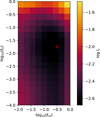 |
Fig. 9 Hyperparameter search for the learning rates of the object and KL modes. |
3.3 Optimization
The loss function of Eq. (17) is simultaneously optimized with respect to the object and the wavefront coefficients using PyTorch, which greatly facilitates the computation of the gradients using automatic differentiation. We note that the weights of the trained SVCE are frozen during this optimization. The optimization is carried out using the AdamW optimizer (Loshchilov & Hutter 2019), very similar to Adam. We verified that using two different learning rates in the AdamW optimizer, one for the objects, ℓo, and one for the KL modes, ℓm, gives excellent results. To find the optimal values of these learning rates, we show in Fig. 9 the loss obtained after 20 epochs for the deconvolution of a 128 × 128 observation from the CRISP instrument at 8542 Å. A clear optimal is found for log10 ℓo ≈ −1.7 and log10 ℓm ≈ −0.5. These values, marked with a red cross in Fig. 9, are used in all our subsequent results.
Our approach can infer the per-pixel wavefront coefficients. In this case, the number of unknowns is X × Y × K for the objects and X × Y × M × L for the wavefront coefficients. As a reminder, X and Y are the spatial dimensions of the images, K is the number of objects, M is the number of KL modes and L is the number of short exposure frames. Using typical values for the parameters, the number of unknowns is of the order of 0.5 M for the objects and 230 M for the wavefront coefficients. In our experiments, the explicit smoothness regularization defined in Eq. (17) seems to be enough. However, we introduce an extra regularization by reducing the number of unknown modes by only inferring the wavefront coefficients in a low-resolution grid, which is a factor P smaller than the original images. The wavefront coefficients in the whole image are computed using bilinear interpolation. In this case, the number of unknowns for the wavefront coefficients is reduced to X/P × Y/P × M × L. Using P = 4, the number of unknowns is reduced to 14.4 M.
The deconvolution can be carried out in the CPU or, ideally, using a GPU. Given the potential limited amount of VRAM (Video Random Access Memory) of current generation of GPUs, it is interesting to apply several well-known techniques to scale our approach to very large images. The first method that we apply is doing all computations in half-precision (FP16), taking advantage of mixed precision training (Micikevicius et al. 2018). The amount of VRAM used is practically halved with respect to using single precision (FP32), with an additional significant reduction in the computation time. In order to avoid numerical underflow, mixed precision training requires to scale the loss function to avoid numerical underflow. The second method that we apply is gradient checkpointing, which trades off VRAM usage for computation time during backpropagation. Backpropagation requires storing intermediate activations for computing gradients during the backward pass, which can be memoryintensive. Instead of storing all activations, only a subset of them are stored. The remaining ones are recomputed on-the-fly during the backward pass. With these techniques, a burst of 20 frames of size 512 × 512 with a single object can be deconvolved using only 8 GB of VRAM. Larger images or a larger number of objects can still be treated using either GPUs with more memory, CPUs (which will make the optimization process typically an order of magnitude slower), or mosaicking.
4 Results
4.1 Reconstructions
We demonstrate in the following the capabilities of our SVCE on reconstructing observations of size 512 × 512. The quality of the reconstruction is shown in Fig. 10 for two observations with CRISP at the SST. The upper panels correspond to the observation of active region AR24473 on 27 Jul. 2020, located at heliocentric coordinates (−20″, −416″). The cadence of the observations is 20 s and a burst of 12 frames is used for the reconstruction. No alignment or destretching is used in this case. The image stability was good so that we assume that spatially variant tip-tilts can be used during the optimization to destretch the images. The lower panels correspond to a quiet Sun observation at disk center, observed on 1 Aug. 2019 with a cadence of 31 s, also composed of a burst of 12 frames. The narrow-band (NB) images (lower rows in each panel) correspond to monochromatic images at 65 mÅ and 130 mÅ from the Ca II 8542 Å chromospheric spectral line. The wide-band images (upper rows in each panel) correspond to the local continuum. We label each image with the value of the contrast, defined as the standard deviation of the image divided by the average. The first column displays ik1, the first frame of the burst, which gives an idea of the quality of the images with the adaptive optics correction. The second column shows ik1 − f ({ok, α1}), the difference between the first frame and the one obtained by convolving the inferred object with the inferred spatially variant PSF. The square of this metric is forced to be zero during the optimization. We quote the NMSE in this column. The third column displays ⟨ikl⟩l=1...L, the average of all frames in the burst. The noise is slightly reduced when compared with a single frame, but the contrast is also reduced. Since the observing conditions were good, the average image is very similar to the first frame. The fourth column shows ![Mathematical equation: $\[o_k^*\]$](/articles/aa/full_html/2024/08/aa49568-24/aa49568-24-eq22.png) , the reconstructed image using the SV-MOMFBD (including filtering), which should be compared with the result of the application of the MOMFBD code (last column). We utilize λo = 0.1 for the sunspot observations and λo = 0.13 for the quiet Sun reconstructions. In both cases, λα = 0.01. A small residual noise is still present in the reconstructions if a smaller λo is used. We optimize the loss function with the AdamW optimizer for 30 iterations. We infer the modes in a grid of 64 × 64, which is a factor 8 smaller than the size of the images. The computing time per iteration is 0.75 s in an NVIDIA RTX 4090 GPU.
, the reconstructed image using the SV-MOMFBD (including filtering), which should be compared with the result of the application of the MOMFBD code (last column). We utilize λo = 0.1 for the sunspot observations and λo = 0.13 for the quiet Sun reconstructions. In both cases, λα = 0.01. A small residual noise is still present in the reconstructions if a smaller λo is used. We optimize the loss function with the AdamW optimizer for 30 iterations. We infer the modes in a grid of 64 × 64, which is a factor 8 smaller than the size of the images. The computing time per iteration is 0.75 s in an NVIDIA RTX 4090 GPU.
Our reconstruction of the active region is able to correctly recover very fine details. The comparison between SV-MOMFBD and MOMFBD is very good. Visually, the contrast is slightly larger in SV-MOMFBD than that found with MOMFBD, which is also quantitatively shown in the figures. The dark cores in the penumbra found in the WB image are recovered visually similarly in both approaches. The same happens for the umbral dots. Concerning the NB images, the contrast is also increased. Despite the similarities, it is true that the SV-MOMFBD reconstruction has some issues. There are some bright regions that are recovered brighter with SV-MOMFBD than with MOMFBD, especially in the NB channel. These regions are indeed present in the individual frames, but they seem to be absent from the MOMFBD reconstruction. Additionally, some small artifacts in the form of rings seem to appear. The dark cores in the penumbra in the NB channel look less straight in SV-MOMFBD than in MOMFBD. The original individual frames seem to contain this feature, which is somehow not absent in MOMFBD. We have not been able to improve them with hyperparameter tuning, so it is clear that more exploration (regularization, improved SVCE, ...) is needed in the near future. Concerning the dark filamentary structure, both reconstructions also produce similar results. The quiet Sun reconstructions are also of very good quality, with contrasts that are slightly larger when using the SV-MOMFBD. Again, the NB images show brighter regions that are not recovered with MOMFBD, although these regions are present in the individual frames. Apart from that, we obtain structures of very similar spatial scales than those found with MOMFBD.
For a more quantitative comparison, we show in Fig. 11 the azimuthally averaged spatial power spectra for the WB channels for the sunspot and quiet Sun observations. The blue curves correspond to individual frames, with the plateau at large wavenumbers produced by the noise. The green and orange curves correspond to the MOMFBD and SV-MOMFBD reconstructions, respectively. The increase in spatial power between 0.02 and 0.3 px−1 is relevant and similar in both reconstructions. This corresponds to the recovery of structures of sizes of between 0.2″ and 3″, which have been destroyed by the seeing. The power spectrum closely follows a power law, strongly reducing the noise for spatial information above 0.3 px−1 when compared to individual frames. The noise reduction abilities of our SV-MOMFBD is very similar to that of MOMFBD. The tiny differences can be associated with the details of the Fourier filtering implemented in both codes. We note a rather abrupt fall of the power above the diffraction limit in SV-MOMFBD. This fall is also visible in MOMFBD, but then the power keeps an almost constant value. This high frequency residual is produced by the stitching of the patches.
The effect of the Tikhonov regularization on the reconstruction is shown in Fig. 12. The first and second columns display the first frames fo the burst for the WB and NB channels, respectively. The impact of the regularization parameter λo (while keeping λα = 0.01) is shown in the third and fourth columns for the WB and NB images, respectively. We note that the spatial frequencies of the reconstruction for λo = 1 are severaly damped, with a significant loss of contrast. However, the reconstruction for λo = 10−3 is more affected by noise. This noise, which has spatial correlation, can trick the eye to produce excessively crispy images. We conclude that a value in the range λo = [0.01, 0.1] seems appropriate for our purposes. Meanwhile, the fifth and sixth columns show the effect of changing the regularization parameter λα (while keeping λo = 0.01). We find that the reconstruction is almost insensitive to the specific value of λα. Anyway, the λo and λα hyperparameters should be taylored for each specific observation and need to be tuned by the user.
Maintaining the photometry is important to keep the polarimetric information after image reconstruction. We show in Fig. 13 the monochromatic Stokes images at 260 mÅ from the line center of the Ca II 8542 Å line. Seeing induced crosstalk can appear given that all modulation states are observed at different times and reconstructed separately. The monochromatic images for all Stokes parameters from the NB camera are obtained after applying the calibrated modulation matrix for SST/CRISP. Our reconstructions and those obtained with MOMFBD are very comparable. We find very similar signals in Stokes V and Stokes U, although larger differences are found for Stokes Q. We also find some noise in the umbra of the sunspot. We checked that this noise decreases as one increases λα. Consequently, we associate the appearance of this noise due to the lack of contrast in the umbra, which make the estimation of the per-pixel wavefront coefficients in these regions uncertain. We defer for the future the analysis of more elaborate regularization techniques to reduce these artifacts. We expect that avoiding the separate reconstruction of all modulated images can help improve the polarimetric capabilities of multiobject multiframe blind deconvolution.
As a final example, the SV-MOMFBD is used for reconstructing observations from the HiFI instrument and the results are displayed in Fig. 14. The observations were acquired on 28 Nov. 2022 at position (226″, −199″), both in Hα and the surrounding continuum. The left panel of Fig. 14 shows the first frame in the first column for the WB and NB channels. A burst of 50 frames taken at a cadence of 100 Hz and an exposure time of 9 ms with a pixel size of 0.050″ is used for the reconstruction. The high-altitude seeing was not very good and quiet large spatially variant tip-tilts are present in the observed frames. For this reason, and given the limited tip-tilts that we used for training the SVCE, we decided to destretch the images similar to what was done by Asensio Ramos et al. (2023). This can be solved in the future by using larger tip-tilts during the training of the SVCE. Our reconstructions (middle column) are compared with those obtained with MOMFBD (right column) using 100 frames with 120 KL modes. Despite the fact that the comparison is not direct, in our opinion, the results with 120 KL modes seem to be a little over-reconstructed, with some artifacts visible in the WB images. This specific reconstruction is obtained with λo = 0.005 and λα = 0.01 and we used a grid of 64×64 pixels for the modes. A Fourier filter with w = 1.85 and n = 20 is used. The quality of the reconstruction depends on the specific hyperparameters used. Although the improvement with respect to individual frames is notable, the comparison is not as satisfactory as those found in Asensio Ramos et al. (2023) and need to be improved in the future. Although the recovered WB contrast is similar to that of MOMFBD, it is clear that we are missing some details, which are more conspicuous in the NB channel. The right panel of Fig. 14 shows the azimuthally averaged spatial power spectra for the WB channels. Both MOMFBD and SV-MOMFBD have a well-defined cut close to the diffraction limit. However, MOMFBD recovers more power at large spatial scales than SV-MOMFBD (between 0.04 and 0.16 px−1, rouhgly equivalent to the range between 6 and 23 px). We are actively working on improving the quality of the reconstructions for HiFI data.
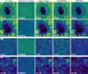 |
Fig. 10 Image reconstruction results for CRISP for a sunspot (upper panels) and a quiet Sun (lower panels) observation. The upper row in each panel shows the results for the wide-band image, while the lower row shows the results for the narrow-band image. The first column shows the first frame in the burst. The second column shows the residual between the first frame and the one obtained by convolving the inferred object with the inferred spatially variant PSF. The third column shows the average of all observed frames. The fourth and fifth columns display the reconstruction with SV-MOMFBD and MOMFBD, respectively. The contrast of the images is quoted in all panels except for those of the second column, which show the NMSE. |
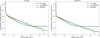 |
Fig. 11 Azimuthally averaged spatial power spectra for the WB channels of the sunspot and quiet Sun observations displayed in Fig. 10. |
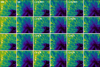 |
Fig. 12 Impact of the hyperparameters for object and modal regularization. The first and second column display the original WB and NB first frames of the burst. The third and fourth columns show the reconstructed WB and NB images, respectively. Each row is labeled by the regularization parameter λo (we use a fixed value of λα = 0.01). The fifth and sixth columns show the reconstructions when the regularization parameter λα is varied (we use a fixed value of λo = 0.01). |
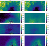 |
Fig. 13 Monochromatic polarimetric images in the NB channel at 260 mÅ from the Ca II 8542 Å line center. |
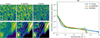 |
Fig. 14 Example of reconstruction of HiFI data (left panel). The first column displays the first images of the burst in the WB and NB channels. The second and third columns show the reconstructed WB and NB images with our SV-MOMFBD and MOMFBD, respectively. The right panel shows the azimuthally averaged spatial power spectra for the WB channels. |
4.2 Modes
Our SV-MOMFBD allows the user to select the grid where the modes are inferred. All previous experiments are carried out with a grid of 64 × 64. As already described, the per-pixel wavefront coefficients required by the SV-MOMFBD are obtained by bilinear interpolation. It is interesting to analyze the impact of using a different grid for the modes. This is shown in Fig. 15, where we show the spatial maps of α1 and α2, the first two KL modes (tip and tilt), from a grid of 8 × 8 up to 128 × 128. All calculations are carried out with the same hyperparameter λα. The first two columns show the reconstructed WB and NB images in each case, respectively. The third and fourth columns show the tip and tilt KL modes for the first frame of the burst, respectively. We note that the inferred tip and tilt are very similar independently of the number of pixels in the grid. Obviously, those with a coarser grid are a coarse representation of those with a finer grid, where tinier details appear. Although the number of unknowns in a factor 256 larger in the finer grid, we do not find any hint of overfitting. Despite the large difference in the number of inferred modes, the reconstructions are all succesful.
It is commonly assumed that it is better to reduce the number of unknowns when solving an inverse problem. This would favor, in our case, using coarse grids. However, we instead follow the philosophy of modeling everything (even if the number of parameters increase much) so that we get close to the limit of inferring almost per-pixel modes and use a much finer grid. With the appropriate regularization that we use (or any other regularization that we can propose in the future), we find no indication of overfitting. Additionally, a significant amount of time is spent in the backpropagation through the bilinear interpolation operator when a coarse grid is used, so that finer grids give much faster reconstructions.
5 Conclusions
The post facto correction of perturbations introduced by the atmosphere when observing with large telescopes is computationally challenging. The small anisoplanatic angles produce PSFs that vary strongly across the FoV. The most commonly used code in the community, MOMFBD, solves this problem by using the OLA method, where reconstructions are carried out in small patches where the PSF is assumed to be constant (and the FFT can be used to carry out convolutions), which are finally stitched together. This approach, although successful, is hampered by several problems. The first is that it cannot be efficiently applied when anisoplanatic patches are very small (in very poor seeing conditions or with very large telescopes). The second problem is that artifacts can appear when stitching together the patches. The MOMFBD code has dealt with this issue fantastically well and these artifacts are barely visible, except in a few exceptional cases. Third, carrying out convolutions using FFT in overlapping patches is not efficient.
In this paper, we show that it is possible to train a deep neural network to emulate convolutions with spatially variant PSFs. The SVCE is able to produce sufficiently good convolutions so that it can be used as a forward model for image reconstruction. The SVCE is fed with an image and a set of images representing the modes of the per-pixel wavefront represented in the KL basis. Although we train the model using spatially invariant convolutions, we verify that the model generalizes correctly to the spatially variant case. The model is very fast and fully convolutional, allowing it to be applied to images of arbitrary size (although the input and output images are of the same size only when the input image has dimensions that are multiples of 24). Apart from the application shown in this paper, there are many other applications that can be explored in the future; of particular relevance is the acceleration of simulations of multiconjugate adaptive optics systems.
We successfully used the SVCE model to obtain a solution for the multiobject, multiframe blind deconvolution problem. The ensuing code, SV-MOMFBD, is able to reconstruct large images at once, also inferring per-pixel PSF. The results displayed in this paper demonstrate that using an SVCE is an interesting way to accelerate image reconstruction for very large telescopes. The reconstructions produced in this study were carried out on standard desktop computers with off-the-shelf GPUs in a matter of tens of seconds for images as large as 512 × 512. This is in opposition to the MOMFBD code, which requires the use of supercomputers. We provide the code for training the SVCE together with the trained model used in the present work, and the code to carry out the multiobject, multiframe blind deconvolution3.
There are a few caveats to the findings presented here. Although the SV-MOMFBD produces good reconstructions, they can be improved to remove artifacts. On one hand, the SVCE model could produce better convolutions. Larger training sets can be built using more images similar to those that can be found in solar observations. One possibility to explore is the use of synthetic observations obtained from radiation magnetohydrodynamical simulations, similar to the line followed by Asensio Ramos & Díaz Baso (2019). Additionally, in order to produce more realistic convolutions, the U-Net model should be forced to produce better results in the point-like objects. This can be achieved by increasing the number of point-like objects in the training set or tweaking the U-Net architecture. We defer these objectives to a future study. On the other hand, the deconvolution implementation shown in this paper lacks many of the technical improvements (phase diversity, pre-alignment of images, removal of polarimetric cross-talk, etc.) implemented in the current version of the MOMFBD code (see Löfdahl et al. 2021, for more details). Adding them will improve the quality of the reconstructions.
Another caveat is that we only explored ℓ2 regularizations for the smoothness of the reconstructed image and the modes. This has given us good results in many reconstructions, but not in all of them. For instance, reconstructing off-limb structures can produce artifacts due to a lack of signal that are arguably better dealt with using other types of regularizations. This problem needs to be explored.
A final caveat is that we used the KL modes as representations of the PSF. Given the presence of ambiguities between wavefronts and PSFs (the same PSF can be obtained with different wavefronts), this representation might not be ideal. We want to explore factorizations extracted empirically from the PSF. One option is to use principal components analysis to extract an orthogonal basis for PSFs (e.g., Lauer 2002), or non-negative matrix factorization (Paatero & Tapper 1994; Lee & Seung 2001) to extract nonorthogonal bases.
The large GPU memory consumption during backpropagation is a problem for reconstructing very large images with our method. Although we used some workarounds, such as working in half-precision and using gradient checkpointing, deconvolving very large bursts of many frames is not yet possible. Possible solutions to this limitation are using multi-GPU architectures or simply working with CPUs.
Finally, we demonstrate that multiobject, multiframe blind deconvolutions can be carried out with SV-MOMFBD using optimization. However, coupling our SVCE with architectures like those explored by Asensio Ramos & Olspert (2021) and Asensio Ramos et al. (2023) will probably produce new advances in speed. In such cases, we can build a larger model composed of a neural network that infers the per-pixel modes from the burst of images and another neural network that infers the reconstructed image. The output of both models can be fed into the SVCE and produce outputs that should be similar to the input burst. This large model can be trained unsupervised. This avenue is of great interest for the deconvolution of observations from solar telescopes of the 4m class, such as the Daniel K. Inouye Solar Telescope (DKIST; Rimmele et al. 2020) and the European Solar Telescope (EST; Quintero Noda et al. 2022).
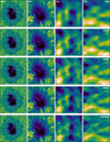 |
Fig. 15 Reconstructions using grids of different number of pixels for the KL modes. The first and second columns display the reconstructed WB and NB images, respectively. The third and fourth columns show the inferred tip and tilts, respectively. |
Acknowledgements
I thank S. Esteban Pozuelo and C. Kuckein for providing the fully reduced SST and GREGOR observations. I also thank Mats Löfdahl for useful discussions. I acknowledge support from the Agencia Estatal de Investigación del Ministerio de Ciencia, Innovación y Universidades (MCIU/AEI) and the European Regional Development Fund (ERDF) through project PID2022-136563NB-I0. This research has made use of NASA’s Astrophysics Data System Bibliographic Services. I acknowledge the community effort devoted to the development of the following open-source packages that were used in this work: numpy (numpy.org, Harris et al. 2020), matplotlib (matplotlib.org, Hunter 2007), and PyTorch (pytorch.org, Paszke et al. 2019).
References
- Asensio Ramos, A., & Díaz Baso, C. J. 2019, A&A, 626, A102 [NASA ADS] [CrossRef] [EDP Sciences] [Google Scholar]
- Asensio Ramos, A., & Olspert, N. 2021, A&A, 646, A100 [NASA ADS] [CrossRef] [EDP Sciences] [Google Scholar]
- Asensio Ramos, A., Esteban Pozuelo, S., & Kuckein, C. 2023, Sol. Phys., 298, 91 [Google Scholar]
- Cornillère, V., Djelouah, A., Yifan, W., Sorkine-Hornung, O., & Schroers, C. 2019, ACM Transac. Graphics, 38, 1 [CrossRef] [Google Scholar]
- Deng, J., Dong, W., Socher, R., et al. 2009, in CVPR09 [Google Scholar]
- Denis, L., Thiébaut, É., Soulez, F., Becker, J.-M., & Mourya, R. 2015, Int. J. Comput. Vision, 115, 253 [CrossRef] [Google Scholar]
- Denker, C. J., Verma, M., Wiśniewska, A., et al. 2023, J. Astron. Telesc. Instrum. Syst., 9, 015001 [NASA ADS] [CrossRef] [Google Scholar]
- Harris, C. R., Millman, K. J., van der Walt, S. J., et al. 2020, Nature, 585, 357 [NASA ADS] [CrossRef] [Google Scholar]
- Hirsch, M., Sra, S., Schölkopf, B., & Harmeling, S. 2010, in Proceedings of the 23rd IEEE Conference on Computer Vision and Pattern Recognition, MaxPlanck-Gesellschaft (Piscataway, NJ, USA: IEEE), 607 [Google Scholar]
- Hunter, J. D. 2007, Comput. Sci. Eng., 9, 90 [NASA ADS] [CrossRef] [Google Scholar]
- Ioffe, S., & Szegedy, C. 2015, in Proceedings of the 32Nd International Conference on International Conference on Machine Learning, 37, 448 [Google Scholar]
- Karhunen, K. 1947, Ann. Acad. Sci. Fennicae. Ser. A. I. Math.-Phys., 37, 1 [Google Scholar]
- Kingma, D. P., & Ba, J. 2014, arXiv e-prints [arXiv:1412.6980] [Google Scholar]
- Lauer, T. R. 2002, in SPIE Astronomical Telescopes + Instrumentation (USA: NASA) [Google Scholar]
- Lee, D., & Seung, H. 2001, Advances in Neural Information Processing Systems, eds. T. K., Leen, T. G., Dietterich, & V., Tresp (Cambridge, Massachusetts: MIT Press) [Google Scholar]
- Loève, M. M. 1955, Probability Theory (Princeton: Van Nostrand Company) [Google Scholar]
- Löfdahl, M. G., & Scharmer, G. B. 1994, A&A, 107, 243 [Google Scholar]
- Löfdahl, M. G., Hillberg, T., de la Cruz Rodríguez, J., et al. 2021, A&A, 653, A68 [Google Scholar]
- Loshchilov, I., & Hutter, F. 2017, in 5th International Conference on Learning Representations, ICLR 2017, Toulon, France, April 24-26, 2017, Conference Track Proceedings (OpenReview.net) [Google Scholar]
- Loshchilov, I., & Hutter, F. 2019, in 7th International Conference on Learning Representations, ICLR 2019, New Orleans, LA, USA, May 6-9, 2019 (OpenReview.net) [Google Scholar]
- Micikevicius, P., Narang, S., Alben, J., et al. 2018, in 6th International Conference on Learning Representations, ICLR 2018, Vancouver, BC, Canada, April 30 - May 3, 2018, Conference Track Proceedings (OpenReview.net) [Google Scholar]
- Molina, R., Nunez, J., Cortijo, F. J., & Mateos, J. 2001, IEEE Signal Process. Magazine, 18, 11 [CrossRef] [Google Scholar]
- Nagy, J. G., & O’Leary, D. P. 1998, SIAM J. Sci. Comput., 19, 1063 [NASA ADS] [CrossRef] [Google Scholar]
- Paatero, P., & Tapper, U. 1994 Environmetrics, 5, 111 [Google Scholar]
- Paszke, A., Gross, S., Massa, F., et al. 2019, in Advances in Neural Information Processing Systems 32, eds. H. Wallach, H. Larochelle, A. Beygelzimer, et al. (UK: Curran Associates, Inc.), 8024 [Google Scholar]
- Perez, E., Strub, F., de Vries, H., Dumoulin, V., & Courville, A. 2017, arXiv e-prints [arXiv:1709.07871] [Google Scholar]
- Quintero Noda, C., Schlichenmaier, R., Bellot Rubio, L. R., et al. 2022, A&A, 666, A21 [NASA ADS] [CrossRef] [EDP Sciences] [Google Scholar]
- Rimmele, T. R., Warner, M., Keil, S. L., et al. 2020, Sol. Phys., 295, 172 [Google Scholar]
- Roddier, N. 1990, Opt. Eng., 29, 1174 [NASA ADS] [CrossRef] [Google Scholar]
- Rombach, R., Blattmann, A., Lorenz, D., Esser, P., & Ommer, B. 2022, in Proceedings of the IEEE Conference on Computer Vision and Pattern Recognition (CVPR) 10684 [Google Scholar]
- Ronneberger, O., Fischer, P., & Brox, T. 2015, arXiv e-prints [arXiv:1505.04597] [Google Scholar]
- Sakai, Y., Yamada, S., Sato, T., et al. 2023, ApJ, 951, 59 [NASA ADS] [CrossRef] [Google Scholar]
- Scharmer, G. 2017, in SOLARNET IV: The Physics of the Sun from the Interior to the Outer Atmosphere, 85 [Google Scholar]
- Scharmer, G. B., Narayan, G., Hillberg, T., et al. 2008, ApJ, 689, L69 [Google Scholar]
- Starck, J. L., Donoho, D. L., Fadili, M. J., & Rassat, A. 2013, A&A, 552, A133 [NASA ADS] [CrossRef] [EDP Sciences] [Google Scholar]
- Stein, R. F. 2012, Liv. Rev. Sol. Phys., 9, 4 [Google Scholar]
- Stein, R. F., & Nordlund, Å. 2012, ApJ, 753, L13 [NASA ADS] [CrossRef] [Google Scholar]
- van Noort, M., Rouppe van der Voort, L., & Löfdahl, M. G. 2005, Sol. Phys., 228, 191 [Google Scholar]
- Zernike, v. F. 1934, Physica, 1, 689 [NASA ADS] [CrossRef] [Google Scholar]
A vector of length I, with a 1 on the component i and zero elsewhere.
All Tables
All Figures
|
Fig. 1 U-Net deep neural network used in the present work as an emulator for the spatially variant convolution. M′ = M + 1 is the number of channels of the input tensor, which is built by concatenating the image of interest and the spatially variant images of the M Karhunen-Loève. All green blocks of the encoder are conditioned to the specific instrumental configuration as described in Sect. 2.2.1 via the encoding fully connected network shown in the figure. The gray box refers to the one-hot encoding of the instrumental configuration. |
| In the text | |
|
Fig. 2 Evolution of training and validation losses for all epochs. The neural network does not show overtraining, although a saturation occurs after epoch ~50. |
| In the text | |
|
Fig. 3 Samples from the training set, showing the capabilities of our model. The upper row displays 12 original images from Stable ImageNet-1K and a synthetic image of point-like objects. The second row displays the target convolved image, with a PSF that is compatible with Kolmogorov turbulence. The third rows shows the output of our model, with the fourth row displaying the residuals. |
| In the text | |
|
Fig. 4 Spatially variant convolution with a defocus obtained with the SVCE. The defocus PSF is shifted along the diagonal of the image. |
| In the text | |
|
Fig. 5 Original image from the Stein (2012) simulation (first panel) together with the image after diffraction when observed with SST/CRISP at 8542 Å (second panel). The third panel displays the spatially variant convolution with a region of defocus computed using per-pixel convolution, with the fourth panel showing the results obtained with the neural SVCE. The last panel displays the residuals, with an NMSE of 1.6 × 10⁻⁴. |
| In the text | |
|
Fig. 6 Computing time per convolution as a function of the size of the image and the batch size for the SVCE, both in CPU and GPU. As a comparison, we show results obtained for the classical method of computing the convolution of the image with a PSF for every pixel. |
| In the text | |
|
Fig. 7 Comparison of the exact PSFs obtained for a specific realization of a Kolmogorov atmosphere with different values of the Fried radius and the neural approximation. Although it captures the general behavior of the PSF, the behavior of the neural model is worse as the level of turbulence increases. Fig. 7. Comparison of the exact PSFs obtained for a specific realization of a Kolmogorov atmosphere with different values of the Fried radius and the neural approximation. Although it captures the general behavior of the PSF, the behavior of the neural model is worse as the level of turbulence increases. |
| In the text | |
|
Fig. 8 Evolution of the NMSE as a function of the Fried radius, showing that the behavior of the neural model worsens when the level of turbulence increases. |
| In the text | |
|
Fig. 9 Hyperparameter search for the learning rates of the object and KL modes. |
| In the text | |
|
Fig. 10 Image reconstruction results for CRISP for a sunspot (upper panels) and a quiet Sun (lower panels) observation. The upper row in each panel shows the results for the wide-band image, while the lower row shows the results for the narrow-band image. The first column shows the first frame in the burst. The second column shows the residual between the first frame and the one obtained by convolving the inferred object with the inferred spatially variant PSF. The third column shows the average of all observed frames. The fourth and fifth columns display the reconstruction with SV-MOMFBD and MOMFBD, respectively. The contrast of the images is quoted in all panels except for those of the second column, which show the NMSE. |
| In the text | |
|
Fig. 11 Azimuthally averaged spatial power spectra for the WB channels of the sunspot and quiet Sun observations displayed in Fig. 10. |
| In the text | |
|
Fig. 12 Impact of the hyperparameters for object and modal regularization. The first and second column display the original WB and NB first frames of the burst. The third and fourth columns show the reconstructed WB and NB images, respectively. Each row is labeled by the regularization parameter λo (we use a fixed value of λα = 0.01). The fifth and sixth columns show the reconstructions when the regularization parameter λα is varied (we use a fixed value of λo = 0.01). |
| In the text | |
|
Fig. 13 Monochromatic polarimetric images in the NB channel at 260 mÅ from the Ca II 8542 Å line center. |
| In the text | |
|
Fig. 14 Example of reconstruction of HiFI data (left panel). The first column displays the first images of the burst in the WB and NB channels. The second and third columns show the reconstructed WB and NB images with our SV-MOMFBD and MOMFBD, respectively. The right panel shows the azimuthally averaged spatial power spectra for the WB channels. |
| In the text | |
|
Fig. 15 Reconstructions using grids of different number of pixels for the KL modes. The first and second columns display the reconstructed WB and NB images, respectively. The third and fourth columns show the inferred tip and tilts, respectively. |
| In the text | |
Current usage metrics show cumulative count of Article Views (full-text article views including HTML views, PDF and ePub downloads, according to the available data) and Abstracts Views on Vision4Press platform.
Data correspond to usage on the plateform after 2015. The current usage metrics is available 48-96 hours after online publication and is updated daily on week days.
Initial download of the metrics may take a while.