| Issue |
A&A
Volume 620, December 2018
|
|
|---|---|---|
| Article Number | A162 | |
| Number of page(s) | 9 | |
| Section | Stellar atmospheres | |
| DOI | https://doi.org/10.1051/0004-6361/201833496 | |
| Published online | 12 December 2018 | |
Mapping EK Draconis with PEPSI★
Possible evidence for starspot penumbrae
Leibniz-Institut für Astrophysik Potsdam (AIP),
An der Sternwarte 16,
14482 Potsdam,
Germany
e-mail: This email address is being protected from spambots. You need JavaScript enabled to view it.
Received:
25
May
2018
Accepted:
13
October
2018
Abstract
Aims. We present the first temperature surface map of EK Dra from very-high-resolution spectra obtained with the Potsdam Echelle Polarimetric and Spectroscopic Instrument (PEPSI) at the Large Binocular Telescope.
Methods. Changes in spectral line profiles are inverted to a stellar surface temperature map using our iMap code. The long-term photometric record is employed to compare our map with previously published maps.
Results. Four cool spots were reconstructed, but no polar spot was seen. The temperature difference to the photosphere of the spots is between 990 and 280 K. Two spots are reconstructed with a typical solar morphology with an umbra and a penumbra. For the one isolated and relatively round spot (spot A), we determine an umbral temperature of 990 K and a penumbral temperature of 180 K below photospheric temperature. The umbra to photosphere intensity ratio of EK Dra is approximately only half of that of a comparison sunspot. A test inversion from degraded line profiles showed that the higher spectral resolution of PEPSI reconstructs the surface with a temperature difference that is on average 10% higher than before and with smaller surface areas by ~10–20%. PEPSI is therefore better suited to detecting and characterising temperature inhomogeneities. With ten more years of photometry, we also refine the spot cycle period of EK Dra to 8.9 ± 0.2 yr with a continuing long-term fading trend.
Conclusions. The temperature morphology of spot A so far appears to show the best evidence for the existence of a solar-like penumbra for a starspot. We emphasise that it is more the non-capture of the true umbral contrast rather than the detection of the weak penumbra that is the limiting factor. The relatively small line broadening of EK Dra, together with the only moderately high spectral resolutions previously available, appear to be the main contributors to the lower-than-expected spot contrasts when comparing to the Sun.
Key words: stars: imaging / stars: activity / starspots / stars: individual: EK Draconis
Based on data acquired with PEPSI using the Large Binocular Telescope (LBT).
© ESO 2018
1 Introduction
EK Draconis (HD 129333, G1.5V) is known as probably the best-studied analogue of the young (≈50 Myr) Sun. Its undepleted lithium abundance, fast rotation, and strong chromospheric and coronal activity are typical for the youth of this star. The target also serves as a corner stone for rotational evolution studies because it is effectively single, bright in X-rays, and accessible to Doppler- and Zeeman-Doppler-imaging studies. No planet has been detected around it so far, but that may be just a question of time. A very good summary of previous observations of this target was given recently by Waite et al. (2017) and we refer the reader to this paper.
Solar analogy taught us that the surface spot distribution is a fingerprint of the underlying dynamo process and its subsequent magnetic-field eruption in form of sunspots or sunspot groups. On stars, we resolve the surface by an indirect tomographic imaging technique called Doppler imaging, and map the surface temperature or brightness distribution as a proxy of the magnetic field. This technique was introduced to cool stars close to 40 yr ago (Vogt & Penrod 1983, see also the review by Strassmeier 2009). It requires high-resolution spectra well sampled over a rotation period of the star but also a target star with rapid rotation so that the line broadening is dominated by Doppler broadening.
Despite the relatively fast rotation of EK Dra with a period of ~2.6 d, the projected rotational velocity on the stellar equator is just ~16 km s−1 . Such small line broadening limits the surface resolution via the Doppler effect and usually brings the instrumental-profile width dangerously close to other thermal and velocity broadening mechanisms like microturbulence (e.g. Collier Cameron 1992; Piskunov & Rice 1993; Rice & Strassmeier 2000). Simulations have shown that a practical limit for the application of the Doppler-imaging technique is reached when there are less thanfive resolution elements across the projected stellar disk (Piskunov & Wehlau 1990) or when the exposure time is so long that the rotational drift is of the same order as the size of the surface feature itself (Collier Cameron 1992). Even with perfect phase coverage and zero microturbulence one can then not reliably reconstruct features, which makes the term imaging eventually obsolete. Therefore, the capability of this technique to resolve stellar surface structure depends on spectral resolution (see also Kürster 1993; Berdyugina et al. 2003).
The first Doppler image of EK Dra was presented by Strassmeier & Rice (1998) based on CFHT/Gecko observations with R = λ∕Δλ = 120 000. It was followed-up with images by Järvinen et al. (2007, 2009) based on NOT/SoFin data with R ≈ 77 000. Instead of temperature maps, two teams have published brightness maps of EK Dra. The brightness maps presented by Rosén et al. (2016) were based on TBL/NARVAL observations with R ≈ 65 000. They reveal larger spots than what is seen in the temperature maps but the locations of the spots in general, ranging from equatorial regions up to higher latitudes, are consistent and comparable. The other set of brightness maps was published just recently by Waite et al. (2017) based on combinations of CFHT/ESPaDOnS (R ≈68 000) and TBL/NARVAL observations. The brightness maps from 2007, produced by the two teams, that is Rosén et al. (2016) and Waite et al. (2017), are similar at the low latitudes, but the map using the first part of the 2007 observations by Waite et al. (2017) shows a prominent high-latitude feature. The latter may have been present also in the map by Rosén et al. (2016), but if so, at somewhat lower latitude. Similarly, the brightness maps from observations in 2012 agree well with each other at low latitudes, but the polar region in the map by Rosén et al. (2016) is featureless while the map by Waite et al. (2017) shows a small but significant polar spot. Such discrepancies are not surprising because at the resolving power of R = 70 000 (4.3 km s−1) one has merely eight resolution elements across the stellar disk. Combined with a non-perfect phase coverage, artefacts will arise from this limitation.
In this paper, we present the first Doppler image employing the very-high-resolution capability of the Potsdam Echelle Polarimetric and Spectroscopic Instrument (PEPSI) at the 2 × 8.4 m (effective aperture of 11.8 m) Large Binocular Telescope (LBT). This enabled a spectral resolution of up to R ≈ 250 000, which translates to approximately 25–30 resolution elements across the stellar disk of EK Dra. The observations are briefly described in Sect. 2. Our Doppler imagery is presented in Sect. 3, while Sect. 4 discusses the results and presents our conclusions.
2 Observations and data reduction
2.1 High-resolution spectroscopy
The spectroscopic observations in this paper were obtained with PEPSI at the 2 × 8.4 m LBT in Arizona. We employed PEPSI’s R = 250 000 mode with seven-slice image slicers and 100 μm fibres. Spectral resolution varies with wavelength (higher in the red, lower in the blue), with position in the échelle order (higher in the centre), and camera-focus position across the CCD (for more details, see Strassmeier et al. 2018a,b, Fig. 3 in both papers). Spectrograph focus during these observations was such that the full width at half maximum (FWHM) of the Th-Ar comparison lines had an average spectral resolution of 230 000 ± 30 000. The instrument is described in detail by Strassmeier et al. (2015).
Monitoring of EK Dra continued over eight nights as part of the instrument commissioning in April 2015. Ten spectra were taken in two wavelength bands simultaneously with cross disperser (CD) III covering 4800–5441 Å and CD V covering 6278–7419 Å.Exposure time was 10 min and typically two back-to-back exposures were obtained and average combined. Average signal-to-noise ratio (S/N) was around 250 per pixel in CD III and 350 in CD V. The logbook of the observations is given in Table 1. Besides the phase-resolved spectra, we also obtained one spectrum in the remaining four CDs of PEPSI. Together with the two CDs from the monitoring, we added these to one phase-averaged (deep) spectrum of EK Dra covering the entire PEPSI format (3837–9140 Å).
Data reduction was done with the software package SDS4PEPSI (“Spectroscopic Data Systems for PEPSI”) based on Ilyin (2000), and described in more detail in Strassmeier et al. (2018a). It relies on adaptive selection of parameters by using statistical inference and robust estimators. The standard reduction steps include bias overscan detection and subtraction, scattered light extraction from the inter-order space and subtraction, definition of échelle orders, optimal extraction of spectral orders, wavelength calibration, and a self-consistent continuum fit to the full two-dimensional (2D) image of extracted orders.
Logbook of the PEPSI observations.
2.2 Photometry
The new photometry was taken with the T7 Amadeus telescope, one of the two 0.75 m Vienna-AIP automatic photoelectric telescopes (APT) at Fairborn Observatory in southern Arizona. Measurements were made differentially between the variable star, a comparison star (HD 129390), a check star (HD 129798), and a sky position using three ten-second integrations. The telescope and photometer themselves are described in Strassmeier et al. (1997b), while the automatic data reduction is described in Strassmeier et al. (1997a) and Granzer et al. (2001). A total of 1138 new Johnson V -band data points are presented covering HJD range 2 454 517–2 457 910 (February 2008–June 2017).
3 Doppler imaging using PEPSI data
3.1 Assumptions
The main assumption comes from knowing the immaculate spectral line profile of the star, that is, the line profile without the surface inhomogeneities that one wants to reconstruct. Our procedure is based on prior local thermodynamic equilibrium (LTE) spectrum synthesis in a wavelength range that is as large as possible with exclusion of spectral regions that are known to be prone to magnetic activity. Besides resonance lines, this excludes optically thick lines, that is, strong and saturated lines with possible chromospheric and/or non-LTE contaminations. In cool stars, also the band heads of TiO and VO molecular series are excluded because of likely (cool) spot contamination. The resulting fit values for effective temperature, gravity, metallicity, and turbulence are then the starting values for our line-profile inversion.
The stellar parameters of EK Dra were first verified with the spectrum synthesis code ParSES (e.g. Allende Prieto et al. 2006) and model atmospheres from MARCS (Gustafsson 2007). We adopted the Gaia-ESO clean line list (Jofré et al. 2014) with various mask widths around the line cores between ±0.05 and ±0.25 Å. As target spectrum, we used the average-combined spectrum from the entire PEPSI data set. This deep spectrum covers the full wavelength range of 3837–9140 Å. Its S/N is inhomogeneous though because the Doppler-imaging monitoring covered ten spectra in CD III+V while the other CDs had only a single observation. The S/N in the CD V, III, VI, and IV ranges therefore peaks at 1000, 600, close to 400, and 250, respectively, and in the bluest part between 100 and 200 (which, however, are not used here). The best ParSES fit leads to Teff = 5730 ± 50 K, log g = 4.41 ± 0.01, [M/H] = −0.2 ± 0.02, ξt = 2.0 ± 0.1 km s−1, and v sin i = 17.5 ± 0.2 km s−1. A recent application to an equivalent PEPSI spectrum of the Sun-as-a-star revealed good agreement with canonical solar values except maybe for v sin i where ParSES preferentially converged on v sin i = 0 ± 1 km s−1 and a microturbulence of 1.2 ± 0.2 km s−1 (see also Strassmeier et al. 2018b). From comparative studies, we would have expected a solar v sin i of 1.9 and a microturbulence of 1.0 or slightly less. It appears that there is remaining cross talk between these two broadening mechanisms at the sub-km s−1 level. However, this will affect the values for EK Dra only at a negligible level because its v sin i ≈17 km s−1 is far beyond the solar value.
Another critical input parameter is the stellar rotation period itself. This is usually best determined from contemporaneous phase-resolved photometry. However, EK Dra’s photometric period appears to change with time. Values between 2.55 and 2.89 d were measured in the past and explained due to spots appearing at different latitudes at different times on a differentially rotating surface (see later Sect. 4). In the present paper, we incorporate differential rotation implicitly in the inversion process by allowing for a latitude-dependent rotation period (actually relative angular velocity). Our assumption is that the angular velocities vary with latitude, θ, only as sin2θ, like on the Sun. We adopt the observed, disk-averaged photometric period of 2.606 d as a starting value.
Dorren & Guinan (1994) estimated the inclination of the rotational axis to be 60° from the photometric period, an average vsini, and an assumed stellar radius of 0.92 R⊙. Line-profile inversions by Strassmeier & Rice (1998) with inclinations between 20° and 90° did indeed result in better fits for i > 55° but did not reveal a particular significant minimum above that limit. This is basically because the Doppler-imaging technique becomes increasingly insensitive to inclination effects once i is above 60°. This exercise was repeated with the current data leading to a refined value of 63° ± 2°.
The well-known bisector shape from surface granulation (e.g. Dravins 2008), which iMap treats in a global manner as a microturbulence broadening in plane-parallel model atmospheres, may in principle also add to the overall residuals. However, the bisector averaged from many hundred lines in the deep spectrum did not show a conclusive deviation from a straight line.
Table 2 summarises the adopted input parameters for our Doppler images.
At this point we note that the Hubble Space Telescope (HST) has witnessed EK Dra having one of the largest far-ultra-violet (FUV) flares ever recorded on a sun-like star (Ayres 2015). Generally, the HST observations show that the outer atmosphere of this star is very complex, energetic, and dynamic (Ayres & France 2010; Ayres 2015). Care must be exercised not to include flare-affected optical spectra for the mapping (see Flores Soriano & Strassmeier 2017; Strassmeier et al. 2018a). No flares were seen in our contemporaneous optical photometry.
Relevant astrophysical properties of EK Dra.
3.2 Inversions
The stellar surface is reconstructed using the iMap code (for details, see Carroll et al. 2007, 2009, 2012). The code can either perform multi-line inversions for a large number of photospheric line profiles simultaneously or use a single average line profile. For the present application, we used a weighted average of 207 spectral lines from wavelength ranges 5000–5400 and 6300–7400 Å with line depths larger than 60% (CD III) and 40% (CD V) of the continuum. Weaker lines were excluded because they decrease rather than increase the S/N. However, for CD V the limit had to be relaxed because there were not enough lines left after applying the original cut-off. The weighted average profiles have S/Ns of ~3500–10 000 per pixel. A total of ten rotational phases fairly equally distributed are available for the inversion.
The rotational phases were calculated from the ephemeris in Eq. (1),
 (1)
(1)
where the period is the average photometric period taken from Järvinen et al. (2005) and the zero point is adopted to be a time of the beginning of the photometric record. We note that a photometric period always reflects the latitude distribution of spots that appeared contemporaneously on the surface of the star. If the star is like the Sun and a differentially rotating body, the true rotation period of the equator will be slightly faster. For high-precision data with high surface resolution, as in this paper, differential rotation may no longer be negligible. Therefore, our Doppler imagery will be done in a comparative way, that is, once with differential surface rotation and once without.
For the line profile computation, iMap solves the radiative transfer with the help of an artificial neural network. The atomic parameters for the line synthesis are taken from the Vienna Atomic Line Database (VALD; Kupka et al. 2011; Ryabchikova et al. 2015). These are used with a grid of Kurucz ATLAS-9 model atmospheres (Castelli & Kurucz 2004) to compute local line profiles in 1D and in LTE. The grid covers temperatures between 3500 and 8000 K in steps of 250 K interpolated to the gravity, metallicity, and microturbulence from the synthesis fits.
For the numerical integration, the stellar surface is partitioned into 5° × 5° segments, resulting in 2592 surface segments for the entire sphere. At the average resolving power of λ∕Δ λ = 230 000, that is, 1.3 km s−1, and an average full width of the lines at a continuum level of 2 (λ∕c) vsini = 0.7 Å (0.54–0.84 Å between 4800 and 7400 Å), we have, on average, an unprecedented 27 resolution elements across the stellar disk. The spherical integration grid samples one spectral resolution element at least with two surface segments when near the stellar equator and near the central meridian. This also means that the integration time shall not exceed 20 min, meaning that phase smearing remains significantly sub-pixel and thus negligible (as a comparison, rotational phase smearing during a 50-min integration as in our CFHT/Gecko data from 1995 amounted to 0. p 013, i.e. of the order of a resolution element of PEPSI).
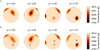 |
Fig. 1 Temperature Doppler images from PEPSI observations. Panel a: based on the original data with a spectral resolution of R = 230 000 on average. Panel b: based on the same data but downgraded to a spectral resolution of 65 000. The spots are labelled A–D. |
3.3 Results
Our surface reconstruction of EK Dra in Fig. 1a reveals three large spots or spot groups and one small feature. These four spots are labelled A–D in Fig. 1b, and their parameters are quantified in Table 3. The spot centres and areas are defined using isothermal contours as described, for example, by Künstler et al. (2015). No warm spots are reconstructed and also no strictly polar feature is seen. The coolest spot, spot A, with a temperature difference of Δ T = 990 K (between unspotted photosphere and spot core) is located on the stellar equator at a phase ϕ = 0.65–0.73. It appears well isolated from the other spots in longitude and latitude. The two larger spots, spots B and C, are at mid-latitudes, ranging approximately from 30° to 60° and appearing with a complex elongated shape. Spot C at ϕ = 0.20–0.30 has a central temperature that is ~700 K cooler than the unspotted surface while spot B at ϕ = 0.85–1.0 appears without any temperature gradient and is only 470 K cooler than the surrounding. The fourth and smallest spot, spot D, is located on the equator at a phase of ϕ = 0.47 with a temperature difference of only ~280 K.
The best line profile fits achieved a χ2 of 4.2 × 10⁻⁴ and are compared with the observations in Fig. 2. This fit approaches the S/N of the weighted average data but does show residuals in the line core with a peak amplitude of ± 3 × 10⁻³. We believe these deviations (Fig. 3) relate to the summed impact from several slightly ill-determined stellar parameters. Other subtle effects like the use of plane-parallel atmospheres in LTE or the magnetic line broadening may contribute at this level. Waite et al. (2017) has shown that EK Dra has a magnetic field with up to approximately ±200 G which has not been taken into account in the local line profiles.
The photospheric temperature was assumed to be the effective temperature and was fixed to 5750 K, which resulted in the overall best fits. From repeated inversions with slightly deviating parameter combinations like, for example, decreased gravity and lowered metallicity (but with always the same line list), we found that the recovered spot temperatures remained surprisingly stable at the ±50 K level. If the parameters become grossly different from what is expected, the code introduces easily recognisable systematic artefacts like dark or bright circum-stellar rings or simply cheats to find a suitable image. We cannot assign an absolute error to each spot’s temperature but state that the errors are likely smaller than 50 K.
In order to quantify the gain from the very-high spectral resolution, we have convolved the PEPSI data with a Gaussian of width proportionalto λ∕Δλ = 65 000, a value usedfor previous EK Dra mappings. However, this does not change the sampling of the data, which means it is an optimistic comparison in favour of the lower resolution spectra. These profiles are then inverted in the same way as the original profiles. The resulting map is presented in Fig. 1b where it can be compared directly with the original map. Its χ2 for the best fit is 3.2 × 10⁻⁴, thus very comparable. The location of the spots are reconstructed almost identically to the high-resolution map; in particular the latitudes, which are typically the quantities the most prone to artefacts. The main difference, however, is that the central (umbral) temperatures of the three larger spots are about 100 K warmer from the lower resolution spectra compared to the map from the higher-resolution spectra. This translates to a full 10%. The weakest spot, spot D, is also found warmer from the lower resolution spectra, but its temperature is only ~50 K higher instead of ~100 K. The second notable difference is that the high-latitude spots B and C appear larger by 19 and 5%, respectively. This causes the two spots to appear almost merged at high latitudes whereas the very-high resolution data led to clearly separated spots. The effect is the opposite for the two small low-latitude spots; spot A appears smaller by 13%, spot D smaller by 33% from the lower resolution spectra.
Spots on EK Dra in April 2015.
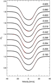 |
Fig. 2 Observed (black dots) and computed (red lines) line profiles for the high-resolution Doppler image in Fig. 1a. Profiles are labelled with their respective rotational phases. Rotation advances from bottom to top. |
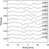 |
Fig. 3 Line profile residuals (observed–inverted). As in Fig. 2, the residual profiles are labeled with their respective phases. The phase-combined rms residual is 4.2 × 10⁻⁴ but systematic deviations appear in individual profiles at ± 3 × 10⁻³. We note that the S/N of the line-averaged data is between 3500 and 10 000 and is thus in the same range as the residuals. |
4 Discussion and conclusions
4.1 Differential surface rotation
Significant differential surface rotation was recently discovered from Stokes V ZDI observations by Waite et al. (2017). Puzzlingly, they had seen no evidence for it from Stokes I. This prompted us to also search for differential rotation (DR) in the (Stokes I) PEPSI data set by applying iMap in its smeared image version. No DR was found in agreement with Waite et al. (2017) although we want to emphasise that almost all of our observations are obtained within one stellar rotation of EK Dra. The question therefore remains as to why one sees DR from Stokes V but not from Stokes I.
We note that the shortest equatorial period, P = 2.51 d, given by Waite et al. (2017) from Stokes V leads to an iMap Stokes I map where the high-latitude spots merge and the smallest spot (D) disappears. Another iMap inversion of our data phased with the longest period from the Stokes V DR fits, P = 2.766 d, leads to a comparable map to our test map in Fig. 1b (which used 2.606 d) but with spot (D) hardly detected. Furthermore, the high-latitude spots appear more elongated than in our 2.606 d map while the central spot regionswere not reconstructed to be as cool as in previous maps. For comparison of the fit qualities, the P = 2.606 d map gave a χ2 of 4.2 × 10⁻⁴ whereas P = 2.51 d gave a χ2 of 5.4 × 10⁻⁴ and P = 2.766 d gave 5.0 × 10⁻⁴, which we consider to be significantly worse than the 2.606-d inversion.
Support for the non-detection of DR from Stokes I comes fromour contemporaneous photometry. For all data sets, P = 2.606 d works reasonable fine, whereas P = 2.51 d and P = 2.766 d do not produce recognisable phase curves at all. We note however that for most observing seasons the entire seasonal data cannot be phased together because of intrinsic changes. A full observing season typically lasts several months. On average we see that the light curves remain stable for one month.
4.2 Spot morphology
The dominating equatorial spot, spot A, appears isolated from the other spotted regions. Therefore, if at all, it is at least minimally affected by cross talk from other spots during the line profile inversion. We chose it for a more detailed analysis. Its morphology (radial temperature profile) is illustrated in Fig. 4. Although the coolest temperature in the centre is covered by only one surface pixel, its neighbouring pixels reach almost the same temperature contrast of ~1000 K. We therefore accept this minimum with confidence. This central region in the spot could be termed its umbra in analogy to sunspot morphology. Consequently, the outer parts could be dubbed the penumbra, appearing on average with an (effective) temperaturecontrast of only 180 K. This is the average of the temperature of the spot’s outer pixel ring compared to the neighbouring photosphere.
While the solar umbra to photosphere intensity ratio is around 0.25, the solar penumbra to photosphere intensity ratio is around 0.80 (e.g. Bray & Loughhead 1964). In terms of effective temperature (at optical depth of 0.67 instead of 1.0 as for the radiation temperature) typical solar penumbrae are cooler by 270 K and umbrae cooler by 1600–2000 K than the photosphere. Compared to a typical sunspot the umbra-to-penumbra contrast on EK Dra appears to be only half of this, as demonstrated in Fig. 5. The lower panel of Fig. 5 compares the radial temperatureprofiles of spot A (reconstructed with two different resolutions) and a Sunspot. The penumbra of spot A is highlighted by the shaded area. We note that in this figure the temperature profiles of both the Sun and EK Dra match the same effective temperature but the EK Dra spot is 27 times larger than the sunspot with a diameter of ~400 Mm based on a stellar radius of EK Dra of 0.98R⊙; the latter is based on the Gaia parallax of 27.90 mas (Gaia Collaboration 2016). There are no such large spots on the Sun. Nevertheless, the stellar spot appears much too warm in its centre compared to its solar counterpart.
We notethat spot C in our map in Fig. 1a also shows an umbra/penumbra morphology but with an even shallower temperaturegradient than spot A. Its central temperature is only 700 K cooler than the photosphere, while its penumbral region is ≈230 K cooler. This makes spot C appear more sun-like in terms of absolute penumbral temperature but its umbral contrast with respect to the photosphere is only about a factor of three, compared to a factor of ~6–7 for our sunspot in Fig. 5. Moreover, spot C is elongated towards spot B and looks more like a big solar active region than a single spot. This suggests a violent interaction between the two features which likely would distort or even fake a penumbral structure. Many smaller unresolved spots between the two features could be an equally likely explanation.Spot A may also be just an unresolved compound of many smaller spots, but it is isolated and relatively circular.
The spectral resolution of all previous data sets of mostly between 65 000 and 77 000 (approximately eight resolution elements across the stellar disk) was likely insufficient to reveal a penumbral structure because the true umbral contrast cannot be captured at this resolution; particularly because EK Dra’s low v sin i is already near the limit that permits the construction of reliable temperature or brightness maps. For example, Mengel et al. (2016) and Waite et al. (2015) unsuccessfully attempted brightness mapping of HD 35296 and τ Boo, both having a comparable vsini of 15 km s−1 but lacking EK Dra’s spot activity.
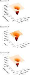 |
Fig. 4 Morphology of spot A (top panel) compared to a sunspot (middle panel). Bottom panel: morphology of spot A when low-resolution data are used. The difference is the weaker umbral region. The x-axis has spot latitude, y-axis has longitude, and z-axis has the temperature elevation. The x- and y-axes of the sunspot (adapted from Balthasar 2006) are in Megameters. |
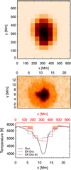 |
Fig. 5 Top panel: iMap reconstruction of spot A. Pixel size is 5° both in longitudinal and in latitudinal direction. The scaling of 27:1 from surface pixels to Megameters is based on a stellar radius of 0.98R⊙. Middle panel: image of an isolated sunspot (adapted from Balthasar 2006). Bottom panel: temperature distribution of the sunspot (black line) in comparison to the mean temperature distribution of spot A of EK Dra (red histogram) and to the low-resolution (lr) result of spot A (grey) histogram). The bins belonging to the penumbra of EK Dra are indicated with light orange colour (shifted by +100 K for better visibility) while the extent of the sunspot penumbra can be directly compared with the middle panel. |
4.3 Comparison to previous maps
To date, five temperature maps and seven brightness maps of EK Dra have been published at rather different epochs. Figure 6 indicates these epochs with respect to the long-term light curve. Because the photometry is best fitted with a periodically modulated long-term variation, which we may call a spot cycle (8.9 yr, see Sect. 4.4), we can identify the cycle phase φ for all DI epochs. The very first temperature map was by Strassmeier & Rice (1998) from data taken in 1995 (φ = 2.19, see Sect. 4.4). Three subsequent maps were made by Järvinen et al. (2007) from data taken in 2001–2002 (from φ =2.91 to φ = 3.03), and another by Järvinen et al. (2009) was made using data taken in 2007.56 (φ = 3.59). The brightness maps by Rosén et al. (2016) were obtained for epochs 2007.1 (φ = 3.53) and 2012.1 (φ = 4.09) and by Waite et al. (2017) for five epochs between 2006 and 2012 (from φ = 3.51 to φ = 4.09).
Thus, maps now cover a full 20-yr period. The surface activity at the times of these maps, indicated by the full photometric amplitude of the rotational modulation, was considerably different. This is illustrated in Fig. 6. During the present mapping season (φ = 4.45) the star showed a peak-to-peak photometric amplitude of up to 0. m13 in V while for example in 2012 (φ = 4.09), during the mapping efforts of Rosén et al. (2016) and Waite et al. (2017), it was roughly half of this. For 2012, Waite et al. (2017) reconstructed a small polar spot on EK Dra (and an even bigger one for January 2008) whereas Rosén et al. (2016) did not recover a polar spot at all. However, the high-latitude feature seen in the maps ranging from the end of 2006 to early 2008 by Waite et al. (2017) is in agreement with the 2007 map presented by Järvinen et al. (2009) which also has a large high-latitude spot reaching a latitude of over 80°. As already discussed by Waite et al. (2017), the mid- to high-latitude spots seem to migrate polewards. Assuming that we see the same high-latitude feature in all these maps, it has a lifetime longer than one year, whereas the low-latitude features appear and disappear within a month. Despite longer lifetimes, the high-latitude spots seem to show evolution (spot coverage, intensity) on a timescale of months. Furthermore, as our latest map shows, the polar region is not covered by spots all the time.
Because DR has only been measured from Stokes V but not from Stokes I, we briefly discuss here the current Zeeman-Doppler imaging (ZDI) literature. The first ZDI maps of EK Dra were published by Rosén et al. (2016). They report mean field strengths of 66 G and 89 G for epochs 2007.1 and 2012.1, respectively. Shortly after that, Waite et al. (2017) published five more ZDI maps of EK Dra, although partially using the same data as Rosén et al. (2016). While Rosén et al. (2016) combined 2007 observations and produced one map, Waite et al. (2017) used those observations separately to create two maps. The 2012 map of both teams is based on the same data set. Waite et al. (2017) reported mean field strengths ranging from 54 to 92 G in agreement with the previous results.
Common to all Doppler maps is the fact that there were always high-latitude and low-latitude spots coexisting, with the high-latitude – sometimes nearly polar – spot always being the more dominant feature. If true and systematic, this would indicate the existence and dominance of a non-axisymmetric dynamo component. However, no signs of a polarity reversal have been detected in the mapping of EK Dra so far (Waite et al. 2017), although one has to note that most of the ZDI maps so far are from the same cycle, only the last one being obtained around the time we assume a new spot cycle has just started (see, Sect. 4.4).
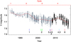 |
Fig. 6 The long-term brightness record of EK Dra. The grey plus symbols denote previously published observations while the open black circles (from 2008 onward) represent new data points from this paper. The red line is the period fit to the data. The upper axis shows the cycle number/phase. The times for which there are published temperature or brightness maps are indicated with vertical ticks as follows: 1: Strassmeier & Rice (1998), 2: Järvinen et al. (2007), 3: Järvinen et al. (2009), 4: Rosén et al. (2016), 5: Waite et al. (2017), and 6: this paper. |
4.4 Long-term photometric behaviour
EK Dra hasbeen photometrically monitored since the year 1958. For the first ~35 yr, the monitoring was done using the Sonneberg Sky-Patrol plates and was analysed by Fröhlich et al. (2002). Strassmeier et al. (1997a) analysed the photometry taken between 1994 and 1996 and reported an average photometric period from those three seasons of 2.605 d, which was interpreted to be the rotation period of EK Dra. They also noted the continuous decrease of the average V light level. Later, Messina & Guinan (2003) analysed the long-term photometric record of the star until 2001 and concluded that the modulation can be fitted by a sinusoid with a period of Pcyc = 9.2 yr plus a longer-term trend (Pcyc ≥ 30 yr if cyclic). They also introduced for the first time a spot cycle for EK Dra, cycle 1 starting around 1984 and lasting until mid-1994. When all of the above data were combined with results from more frequent monitoring (Järvinen et al. 2005, 2009), it was obvious that the star had been getting fainter for a time period of ~50 yr, with some additional periodic variation of ~10.5 yr. Adding eight more years of observations (Fig. 6) does not yet confirm that the star has reached the minimum magnitude. For some time it looked as though there was a minimum around 2006/2007. However, the latest photometry confirmed that this was only a local and not a global minimum.
We have prewhitened the entire photometric record with the long-term trend of 60+ yr and refine the period to 8.9 ± 0.2 yr. The fit to the observations with the long-term cycle trend is shown in Fig. 6. The refined period is close to the period originally obtained by Messina & Guinan (2003) and is similar to the solar 11-yr sunspot cycle, while the long-term trend indicates the presence of a cycle that may be similar to the solar Gleissberg cycle.
With the 8.9-yr period, we can see that the photometric record in Fig. 6 already covers over four cycles. Cycle 1 started 1984.6, in agreement with the definition given by Messina & Guinan (2003), corresponding to the time of photometricmaximum (i.e. the smallest number of spots on the stellar surface). The first modern photometric observations (in late 1983) were taken at the end of cycle 0, just before cycle 1 began. Based on the period of 8.9 yr, cycle 0 must have started around 1975.7, and indeed, the analysis by Fröhlich et al. (2002) indicated that there was a photometric maximum around that time.
5 Summary
In this paper, we present the first temperature map based on very-high-resolution spectra obtained with PEPSI at LBT. We show that the relatively small line broadening of EK Dra, together with the only moderately high spectral resolutions previously available, appear to be among the main contributors to the lower-than-expected spot contrasts when comparing to the Sun. A test inversion from degraded line profiles shows that the higher spectral resolution of PEPSI reconstructs the surface with a 10% higher temperature difference (on average) than before and with smaller surface areas by ~10–20%.
The reconstructed stellar surface has four spots with temperature differences between 990 and 280 K below the photospheric temperature (5730 ± 50 K). Two of the spots are reconstructed with a typical solar morphology with an umbra and a penumbra. For the one isolated and relatively round spot (spot A), we determine an umbral temperature of 990 K cooler than the unspotted photosphere, whereas the penumbra is only 180 K cooler. This leads to an umbra to photosphere intensity ratio that is approximately only half of that of our comparison sunspot. Spot A of EK Dra is 27 times larger than this comparison sunspot, and has a diameter of ~400 Mm. There are no such large spots on the Sun, but the EK Dra spot still appears much too warm in its centre compared to its solar counterpart. We do not yet see evidence for a conglomerate of little spots.
From the photometric record now covering almost 40 yrs, we have refined a spot cycle period to 8.9 ± 0.2 yr. Additionally, the photometry reveals that the star still continues to fade.
Acknowledgements
We thank the anonymous referee for careful reading of the manuscript and very helpful comments. The LBT is an international collaboration among institutions in the United States, Italy, and Germany. LBT Corporation partners are the University of Arizona on behalf of the Arizona university system; Istituto Nazionale di Astrofisica, Italy; LBT Beteiligungsgesellschaft, Germany, representing the Max-Planck Society, the Leibniz-Institute for Astrophysics Potsdam (AIP), and Heidelberg University; the Ohio State University; and the Research Corporation, on behalf of the University of Notre Dame, University of Minnesota, and University of Virginia. It is a pleasure to thank the German Federal Ministry (BMBF) for the year-long support for the construction of PEPSI through their Verbundforschung grants 05AL2BA1/3 and 05A08BAC as well as the State of Brandenburg for the continuing support of AIP and PEPSI in particular (see https://pepsi.aip.de/). This work has made use of the VALD database, operated at Uppsala University, the Institute of Astronomy RAS in Moscow, and the University of Vienna. This research has made use of NASA’s Astrophysics Data System and of CDS’s Simbad database.
References
- Allende Prieto, C., Beers, T. C., Wilhelm, R., et al. 2006, ApJ, 636, 804 [NASA ADS] [CrossRef] [Google Scholar]
- Ayres, T. R. 2015, in Amer. Astron. Soc. Meet. Abstr., 225, 138.23 [Google Scholar]
- Ayres, T., & France, K. 2010, ApJ, 723, L38 [NASA ADS] [CrossRef] [Google Scholar]
- Balthasar, H. 2006, A&A, 449, 1169 [NASA ADS] [CrossRef] [EDP Sciences] [Google Scholar]
- Berdyugina, S. V., Telting, J. H., & Korhonen, H. 2003, A&A, 406, 273 [NASA ADS] [CrossRef] [EDP Sciences] [Google Scholar]
- Bray, R. J., & Loughhead, R. E. 1964, Sunspots (London: Chapman and Hall) [Google Scholar]
- Carroll, T. A., Kopf, M., Ilyin, I., & Strassmeier, K. G. 2007, Astron. Nachr., 328, 1043 [NASA ADS] [CrossRef] [Google Scholar]
- Carroll, T. A., Kopf, M., Strassmeier, K. G., & Ilyin, I. 2009, in IAU Symp., 259, 633 [Google Scholar]
- Carroll, T. A., Strassmeier, K. G., Rice, J. B., & Künstler, A. 2012, A&A, 548, A95 [NASA ADS] [CrossRef] [EDP Sciences] [Google Scholar]
- Castelli, F., & Kurucz, R. L. 2004, ArXiv Astrophysics e-prints [astro-ph/0405087] [Google Scholar]
- Collier Cameron, A. 1992, in Surface Inhomogeneities on Late-Type Stars, ed. P. B. Byrne & D. J. Mullan, Lect. Notes Phys. (Berlin: Springer Verlag), 397, 33 [NASA ADS] [CrossRef] [Google Scholar]
- Dorren, J. D.,& Guinan, E. F. 1994, ApJ, 428, 805 [NASA ADS] [CrossRef] [Google Scholar]
- Dravins, D. 2008, A&A, 492, 199 [NASA ADS] [CrossRef] [EDP Sciences] [Google Scholar]
- Flores Soriano, M., & Strassmeier, K. G. 2017, A&A, 597, A101 [NASA ADS] [CrossRef] [EDP Sciences] [Google Scholar]
- Fröhlich, H.-E., Tschäpe, R., Rüdiger, G., & Strassmeier, K. G. 2002, A&A, 391, 659 [NASA ADS] [CrossRef] [EDP Sciences] [Google Scholar]
- Gaia Collaboration (Brown, A. G. A., et al.) 2016, A&A, 595, A2 [NASA ADS] [CrossRef] [EDP Sciences] [Google Scholar]
- Granzer, T., Reegen, P., & Strassmeier, K. G. 2001, Astron. Nachr., 322, 325 [NASA ADS] [CrossRef] [Google Scholar]
- Gustafsson, B. 2007, in Why Galaxies Care About AGB Stars: Their Importance as Actors and Probes, eds. F. Kerschbaum, C. Charbonnel, & R. F. Wing, ASP Conf. Ser., 378, 60 [NASA ADS] [Google Scholar]
- Ilyin, I. V. 2000, Ph.D. Thesis, University of Oulu Finland [Google Scholar]
- Järvinen, S. P., Berdyugina, S. V., & Strassmeier, K. G. 2005, A&A, 440, 735 [NASA ADS] [CrossRef] [EDP Sciences] [Google Scholar]
- Järvinen, S. P., Berdyugina, S. V., Korhonen, H., Ilyin, I., & Tuominen, I. 2007, A&A, 472, 887 [NASA ADS] [CrossRef] [EDP Sciences] [Google Scholar]
- Järvinen, S. P., Korhonen, H., Berdyugina, S. V., & Ilyin, I. 2009, in 15th Cambridge Workshop on Cool Stars, Stellar Systems, and the Sun, ed. E. Stempels, AIP Conf. Ser., 1094, 660 [Google Scholar]
- Jofré, P., Heiter, U., Soubiran, C., et al. 2014, A&A, 564, A133 [NASA ADS] [CrossRef] [EDP Sciences] [Google Scholar]
- Künstler, A., Carroll, T. A., & Strassmeier, K. G. 2015, A&A, 578, A101 [NASA ADS] [CrossRef] [EDP Sciences] [Google Scholar]
- Kupka, F., Dubernet, M.-L., & VAMDC Collaboration 2011, Balt. Astron., 20, 503 [Google Scholar]
- Kürster, M. 1993, A&A, 274, 851 [NASA ADS] [Google Scholar]
- Mengel, M. W., Fares, R., Marsden, S. C., et al. 2016, MNRAS, 459, 4325 [NASA ADS] [CrossRef] [Google Scholar]
- Messina, S., & Guinan, E. F. 2003, A&A, 409, 1017 [NASA ADS] [CrossRef] [EDP Sciences] [Google Scholar]
- Piskunov, N. E., & Rice, J. B. 1993, PASP, 105, 1415 [NASA ADS] [CrossRef] [Google Scholar]
- Piskunov, N. E., & Wehlau, W. H. 1990, A&A, 233, 497 [NASA ADS] [Google Scholar]
- Rice, J. B., & Strassmeier, K. G. 2000, A&AS, 147, 151 [NASA ADS] [CrossRef] [EDP Sciences] [Google Scholar]
- Rosén, L., Kochukhov, O., Hackman, T., & Lehtinen, J. 2016, A&A, 593, A35 [NASA ADS] [CrossRef] [EDP Sciences] [Google Scholar]
- Ryabchikova, T., Piskunov, N., Kurucz, R. L., et al. 2015, Phys. Scr., 90, 054005 [NASA ADS] [CrossRef] [Google Scholar]
- Strassmeier, K. G. 2009, A&ARv, 17, 251 [NASA ADS] [CrossRef] [Google Scholar]
- Strassmeier, K. G., & Rice, J. B. 1998, A&A, 330, 685 [NASA ADS] [Google Scholar]
- Strassmeier, K. G., Bartus, J., Cutispoto, G., & Rodono, M. 1997a, A&AS, 125, 11 [NASA ADS] [CrossRef] [EDP Sciences] [Google Scholar]
- Strassmeier, K. G., Boyd, L. J., Epand, D. H., & Granzer, T. 1997b, PASP, 109, 697 [NASA ADS] [CrossRef] [Google Scholar]
- Strassmeier, K. G., Ilyin, I., Järvinen, A., et al. 2015, Astron. Nachr., 336, 324 [NASA ADS] [CrossRef] [Google Scholar]
- Strassmeier, K. G., Ilyin, I., & Steffen, M. 2018a, A&A, 612, A44 [NASA ADS] [CrossRef] [EDP Sciences] [Google Scholar]
- Strassmeier, K. G., Ilyin, I., & Weber, M. 2018b, A&A, 612, A45 [NASA ADS] [CrossRef] [EDP Sciences] [Google Scholar]
- Vogt, S. S., & Penrod, G. D. 1983, PASP, 95, 565 [NASA ADS] [CrossRef] [Google Scholar]
- Waite, I. A., Marsden, S. C., Carter, B. D., et al. 2015, MNRAS, 449, 8 [NASA ADS] [CrossRef] [Google Scholar]
- Waite, I. A., Marsden, S. C., Carter, B. D., et al. 2017, MNRAS, 465, 2076 [NASA ADS] [CrossRef] [Google Scholar]
All Tables
All Figures
|
Fig. 1 Temperature Doppler images from PEPSI observations. Panel a: based on the original data with a spectral resolution of R = 230 000 on average. Panel b: based on the same data but downgraded to a spectral resolution of 65 000. The spots are labelled A–D. |
| In the text | |
|
Fig. 2 Observed (black dots) and computed (red lines) line profiles for the high-resolution Doppler image in Fig. 1a. Profiles are labelled with their respective rotational phases. Rotation advances from bottom to top. |
| In the text | |
|
Fig. 3 Line profile residuals (observed–inverted). As in Fig. 2, the residual profiles are labeled with their respective phases. The phase-combined rms residual is 4.2 × 10⁻⁴ but systematic deviations appear in individual profiles at ± 3 × 10⁻³. We note that the S/N of the line-averaged data is between 3500 and 10 000 and is thus in the same range as the residuals. |
| In the text | |
|
Fig. 4 Morphology of spot A (top panel) compared to a sunspot (middle panel). Bottom panel: morphology of spot A when low-resolution data are used. The difference is the weaker umbral region. The x-axis has spot latitude, y-axis has longitude, and z-axis has the temperature elevation. The x- and y-axes of the sunspot (adapted from Balthasar 2006) are in Megameters. |
| In the text | |
|
Fig. 5 Top panel: iMap reconstruction of spot A. Pixel size is 5° both in longitudinal and in latitudinal direction. The scaling of 27:1 from surface pixels to Megameters is based on a stellar radius of 0.98R⊙. Middle panel: image of an isolated sunspot (adapted from Balthasar 2006). Bottom panel: temperature distribution of the sunspot (black line) in comparison to the mean temperature distribution of spot A of EK Dra (red histogram) and to the low-resolution (lr) result of spot A (grey) histogram). The bins belonging to the penumbra of EK Dra are indicated with light orange colour (shifted by +100 K for better visibility) while the extent of the sunspot penumbra can be directly compared with the middle panel. |
| In the text | |
|
Fig. 6 The long-term brightness record of EK Dra. The grey plus symbols denote previously published observations while the open black circles (from 2008 onward) represent new data points from this paper. The red line is the period fit to the data. The upper axis shows the cycle number/phase. The times for which there are published temperature or brightness maps are indicated with vertical ticks as follows: 1: Strassmeier & Rice (1998), 2: Järvinen et al. (2007), 3: Järvinen et al. (2009), 4: Rosén et al. (2016), 5: Waite et al. (2017), and 6: this paper. |
| In the text | |
Current usage metrics show cumulative count of Article Views (full-text article views including HTML views, PDF and ePub downloads, according to the available data) and Abstracts Views on Vision4Press platform.
Data correspond to usage on the plateform after 2015. The current usage metrics is available 48-96 hours after online publication and is updated daily on week days.
Initial download of the metrics may take a while.