| Issue |
A&A
Volume 620, December 2018
|
|
|---|---|---|
| Article Number | A139 | |
| Number of page(s) | 15 | |
| Section | Planets and planetary systems | |
| DOI | https://doi.org/10.1051/0004-6361/201833123 | |
| Published online | 10 December 2018 | |
Incidence of planet candidates in open clusters and a planet confirmation★,★★
1
Departamento de Física, Universidade Federal do Rio Grande do Norte,
59078-970
Natal, RN,
Brazil
e-mail: This email address is being protected from spambots. You need JavaScript enabled to view it.
2
Observatoire de Genève,
Université de Genève,
51 Ch. des Maillettes, 1290 Sauverny, Switzerland
3
Universidade Federal do Recôncavo da Bahia, Centro de Ciências Exatas e Tecnológicas, Av. Rui Barbosa, 710,
Cruz das Almas, BA,
44380-000,
Brazil
4
Departamento de Física, Facultad de Ciencias Básicas, Universidad Metropolitana de la Educación, Av. José Pedro Alessandri 774, 7760197 Nuñoa,
Santiago, Chile
5
Millennium Institute of Astrophysics,
Santiago, Chile
6
European Southern Observatory,
Karl-Schwarzschild-Straße 2,
85748 Garching bei München, Germany
7
ESO,
Casilla 19001,
Santiago 19, Chile
8
Departamento de Física, Universidade Federal do Ceará,
Caixa Postal 6030, Campus do Pici, 60455-900 Fortaleza,
Ceará, Brazil
Received:
28
March
2018
Accepted:
7
July
2018
Abstract
Context. Detecting exoplanets in clusters of different ages is a powerful tool for understanding a number of open questions, such as how the occurrence rate of planets depends on stellar metallicity, on mass, or on stellar environment.
Aims. We present the first results of our HARPS long-term radial velocity (RV) survey which aims to discover exoplanets around intermediate-mass (between ~2 and 6 M⊙) evolved stars in open clusters.
Methods. We selected 826 bona fide HARPS observations of 114 giants from an initial list of 29 open clusters and computed the half-peak to peak variability of the HARPS RV measurements, namely ΔRV∕2, for each target, to search for the best planet-host candidates. We also performed time series analyses for a few targets for which we have enough observations to search for orbital solutions.
Results. Although we attempted to rule out the presence of binaries on the basis of previous surveys, we detected 14 new binary candidates in our sample, most of them identified from a comparison between HARPS and CORAVEL data. We also suggest 11 new planet-host candidates based on a relation between the stellar surface gravity and ΔRV∕2. Ten of the candidates are less than 3 M⊙, showing evidence of a low planet occurrence rate for massive stars. One of the planet-host candidates and one of the binary candidates show very clear RV periodic variations, allowing us to confirm the discovery of a new planet and to compute the orbital solution for the binary. The planet is IC 4651 9122b, with a minimum mass of m sini = 6.3 MJ and a semimajor axis a = 2.0 AU. The binary companion is NGC 5822 201B, with a very low minimum mass of m sini = 0.11 M⊙ and a semimajor axis a = 6.5 AU, which is comparable to the Jupiter distance to the Sun.
Key words: planetary systems / open clusters and associations: general / stars: late-type / binaries: spectroscopic / techniques: radial velocities
Based on observations collected with the 3.6 m Telescope (La Silla Observatory, ESO, Chile) using the HARPS instrument (programs ID: 091.C-0438, 092.C-0282, and 094.C-0297).
The reduced time series data are only available at the CDS via anonymous ftp to cdsarc.u-strasbg.fr (130.79.128.5) or via http://cdsarc.u-strasbg.fr/viz-bin/qcat?J/A+A/620/A139
© ESO 2018
1 Introduction
After the pioneering discovery of the giant planet orbiting 51 Peg by Mayor & Queloz (1995), two decades ago, to date the literature1 reports the discovery of more than 3700 planets, in about 2800 planetary systems. Solar stars in the field host the vast majority of these exoplanets. The characteristics of field stars may represent a drawback for our capability to derive precise conclusions to very basic questions. For example, more than 70% of the known planets orbit stars with masses M* < 1.30 M⊙. Our understanding of planet formation as a function of the mass of the host star and of the stellar environments is therefore still poorly understood. In addition, it has been observed that main sequence stars hosting giant planets are metal-rich (Gonzalez 1997; Santos et al. 2004), while evolved stars hosting giant planets are likely not (Pasquini et al. 2007; see, however, for different conclusions Jones et al. 2016). There is no clear explanation for this discrepancy, and several competing scenarios have been proposed. These scenarios include stellar pollution acting on main-sequence stars (e.g., Laughlin & Adams 1997), a planet formation (core-accretion) mechanism favoring the birth of planets around metal-rich stars (Pollack et al. 1996), and an effect of stellar migration (radial mixing) in the Galactic disk (Haywood 2009).
Open cluster stars formed simultaneously from a single molecular cloud with uniform physical properties, and thus have the same age, chemical composition and galactocentric distance. As a result, these are valuable testbeds for studying how the planet occurrence rate depends on stellar mass and environment. Furthermore, comparing homogeneous sets of open-cluster stars with and without planets is an ideal method for determining whether thepresence of a planetary companion alters the chemical composition of the host stars (e.g., Israelian et al. 2009).
The number of planetary mass companions discovered around open cluster stars is rapidly growing, amounting to date to 25 planets. Two hot-Jupiters and a massive outer planet in the Praesepe open cluster (Quinn et al. 2012; Malavolta et al. 2016), a hot-Jupiter in the Hyades (Quinn et al. 2014), two sub-Neptune planets in NGC 6811 (Meibom et al. 2013), five Jupiter-mass planets in M67 (Brucalassi et al. 2014, 2016, 2017), a Neptune-sized planet transiting an M4.5 dwarf in the Hyades (Mann et al. 2016; David et al. 2016), three Earth-to-Neptune-sized planets around a mid-K dwarf in the Hyades (Mann et al. 2018), a Neptune-sized planet orbiting an M dwarf in Praesepe (Obermeier et al. 2016) and eight planets from K2 campaigns (Pope et al. 2016; Barros et al. 2016; Libralato et al. 2016; Mann et al. 2017; Curtis et al. 2018), have been recently reported. Three planet candidates were also announced in the M67 field (Nardiello et al. 2016), although all the host stars appear to be non-members. Previous radial velocity studies focusing on evolved stars revealed a giant planet around one of the Hyades clump giants (Sato et al. 2007) and a substellar-mass object in NGC 2423 (Lovis & Mayor 2007). These studies confirm that giant planets around open cluster stars exist and can probably migrate in a dense cluster environment. Meibom et al. (2013) found that the properties and occurrence rate of low mass planets are the same in open clusters and field stars. Finally, the radial velocity (RV) measurements of M67 show that the occurrence rate of giant planets is compatible with that observed in field stars (~ 16%), albeit with an excess of hot jupiters in this cluster (Brucalassi et al. 2016).
These studies demonstrate the wealth of information which can be gained from open clusters, which has so far been limited to solar mass stars. It is necessary to extend the work to a broader range of stellar masses and ages for a better understanding about the planet occurrence rate related with the mass, environment, and chemical composition of the host stars. However, more massive hot stars show very few spectral lines, which are all broad. As a result, cool stars in the red giant region are excellent candidates for extending these works to higher masses (Setiawan et al. 2004; Johnson et al. 2007).
Over the past three years we have carried out a search for massive planets around 152 evolved stars belonging to 29 open clusters. From these clusters we selected 114 targets with the best quality data and with a minimum of two observations per target, as described in Sect. 2.2. These targets were relatively well studied for duplicity, and also with good constraints for mass, composition and age determinations. Our survey aims to estimate the planet occurrence rate of intermediate-mass late-type giant stars in young and intermediate-age open clusters. This paper provides an overview (as made in Pasquini et al. 2012 for M67) of the stellar sample and the observations, discussing the clusters’ characteristics and the RV distribution of the stars, and highlighting the most likely planetary host candidates. The paper is structured as follows. The observations, sample selection, and methods used in our analysis are described in Sect. 2. Several results are presented in Sect. 3, including a detailed overview of the data we have collected so far, combined with observations of other programs, and the discovery of a new planet. Finally, we state our conclusions in Sect. 4.
2 Working sample, observations, and methods
The stellar sample was selected from Mermilliod et al. (2008), who determined cluster membership and binaries using CORAVEL. The stellar B and V magnitudes, Bmag and Vmag, were obtained from the Simbad2 database, from which we also computed the (B−V) color index. Absolute magnitudes, MV, were estimated from Vmag and the cluster distance modulus obtained from Kharchenko et al. (2005) and from the WEBDA3 cluster database (Mermilliod 1995). Both (B−V) and MV were corrected for reddening, E(B−V), from Wu et al. (2009). Cluster ages were taken from Wu et al. (2009) and metallicities from Wu et al. (2009) and Heiter et al. (2014).
The main cluster selection criteria were the age of the cluster (between 0.02 and ~2 Gyr, with turnoff masses ≳ 2 M⊙) and the apparent magnitude of the giant stars (brighter than Vmag ~ 14 mag). We then rejected cool, bright stars with (B−V) > 1.4 as these are known to be RV unstable (e.g., Hekker et al. 2006). Known binaries and non-members were removed from the sample. We note that we picked up only the clusters with at least two giant members each and that the chosen open clusters span a rather narrow metallicity range (about − 0.2 < [Fe∕H] < 0.2). Seven clusters were in common with Lovis & Mayor (2007). To first order, we assumed that all giants in a given cluster have the same mass, which is approximately the mass at the main-sequence turnoff.
2.1 HARPS observations
The High Accuracy Radial velocity Planet Searcher4 (HARPS; Mayor et al. 2003) is the planet hunter at the ESO 3.6 m Telescope in La Silla. In high accuracy mode (HAM), it has an aperture on the sky of one arcsecond, and a resolving power of 115 000. The spectral range covered is 380–680 nm. In addition to be exceptionally stable, HARPS achieves the highest precision using the simultaneous calibration principle: the spectrum of a calibration (Th-Ar) source is recorded simultaneously with the stellar spectrum, with a second optical fiber. As a rule of thumb, we can consider the precision of HARPS scales as  , where ϵRV is the RV photon-noise error and S/N is the signal-to-noise ratio. An ϵRV of a few m s−1 (~10 m s−1 or better) is possible with limited S/N observations, namely at least S∕N ~ 10. In practice, our observed HARPS spectra have typically a peak S/N of 10–20 for the faintest stars and of 50–100 for the brightest ones. HARPS is equipped with a very powerful pipeline (Mayor et al. 2003) that provides online RV measurements, which are computed by cross-correlating the stellar spectrum with a numerical template mask. This online pipeline also provides an associated ϵRV. For all of our stars, irrespective of the spectral type and luminosity, we used the solar template (G2V) mask.
Between April 4, 2013 and April 1, 2015 we obtained 500 observations of 152 targets with HARPS spread over our 29 open clusters. We then combined these data with 494 more HARPS observations of stars that were in our sample and collected using the same G2V mask, all available in the ESO Archive. This provided a total of 994 observations for these targets obtained with a decade-long baseline, from 2005 to 2015, from which we selected our final sample of 826 effective observations of 114 stars, as described in Sect. 2.2. Table 1 lists the stars by cluster, with the initial number of objects and observations considered in this work.
Number of observed stars (Nobj) of our original list of 29 open clusters and total number of HARPS observations (Nobs) carried out by our and other programs for each cluster.
2.2 Finalsample
The HARPS pipeline usually produces very good quality data from a fully automatic process. However, a visual inspection of the reduced data is required to remove outliers caused by a variety of different issues (bad observation conditions and erroneous reduction, amongst others). Therefore, we performed a visual inspection of all the 994 HARPS observations described in Sect. 2.1 and, for a few cases, we rereduced the data manually by using the offline tools of the HARPS pipeline to correct reduction issues.
We discarded 18 spectra with S/N below 10, and nine spectra with problematic cross-correlation function (CCF) shape. Finally, we merged observations separated by less than 3 days by averaging all the reduced parameters (time, RV, bisector velocity span, and S/N). This averaging tends to clean up short-period variations (likely produced by intrinsic stellar signal) and keeps periods longer than ~10 days, whichcorrespond, for the stellar mass range of our sample (~2–6 M⊙), to planetary semimajor axes ≳0.1 AU (i.e., a threshold comparable to the typical radii of giant stars, below which inner planet orbits are not expected in our sample). From the remaining data, we required at least two observations per target to analyze the RV distributions as described below. This final sample comprises a total of 826 effective observations of 114 targets. Figure 1 shows the distribution of ϵRV vs. S/N for our sample, with objects belonging to different criteria in the refinement to final sample highlighted by different symbols.
2.3 Activity proxy measurements
The bisector velocity span (or simply bisector span) is a measurement of the CCF asymmetry computed from the CCF bisector (which is the set of midpoints between the two sides of a CCF profile) at the top and bottom of the CCF profile (e.g., Queloz et al. 2001). It is a standard output of the HARPS pipeline and an important stellar activity proxy which is used to verify whether an RV variation is caused by intrinsic stellar variability (e.g., induced by chromospheric activity) rather than by orbital motion. It has been demonstrated that, in the case of activity-induced RV variations, these correlate with the bisector span variations (e.g., Santos et al. 2002).
Another important stellar activity proxy is the S index, obtained from the emission in the core of the CaII H & K spectral lines. It is a dimensionless quantity typically measured from the total flux counts of two triangular passbands 1.09 Å wide centered at 3933.66 Å (the CaII K line) and at 3968.47 Å (the CaII H line) and normalized by the total flux of two continuum passbands 20 Å wide centered at 3901.07 Å (a pseudo blue filter) and 4001.07 Å (a pseudo red filter; e.g., Schröder et al. 2009). The S index is, thus, defined as
 (1)
(1)
where H, K, R, and V are the total flux counts of the pseudo-filters described above and α is a factor for instrumental calibration. We measured this index by using the reduced HARPS spectra, which is also provided by the pipeline, but no instrumental calibration was performed (ie., we assumed α = 1) because we are only interested in the index variation. This index, as the bisector span, should not correlate with RV if the RV variation has an orbital origin, and it is reliable only for observations with high S/N (e.g., S∕N ≳ 21 at 400 nm; see Sect. 3.4).
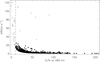 |
Fig. 1 Photon noise error in the measurement of the CCF center of single observations vs. S/N at 490 nm for our sample of open cluster targets observed with HARPS. The overall RV errors are typically distributed around 1–4 m s−1 and range from 42 cm s−1 to 119 m s−1. The overall S/N distribution peaks around 20–40 and ranges from 2.4 to 223. Black filled circles are the selected data, and gray crosses are the discarded ones, all identified from a visual inspection of the CCFs. Black open circles depict the data with S∕N < 10 that were also discarded and this threshold is represented by the vertical dashed line. |
2.4 Planet-host candidate selection method
A reasonable selection of planet-host candidates can be obtained by using the relation described in Hekker et al. (2008). Based on a sample of K giants, these authors found a trend where the RV semiamplitude increases with the decreasing logarithm of stellar surface gravity, log g. This trend may arise from intrinsic RV variability induced by stellar oscillation (Kjeldsen & Bedding 1995), and was also observed by other groups (e.g., Setiawan et al. 2004). Planet-host candidates can be identified as those with RV lying noticeably above the trend.
Troup et al. (2016) follow this approach to search for exoplanets using data from APOGEE5 (Majewski et al. 2017), with a pre-selection criterion quantified by their Eqs. (25)–(27). At first order, these equations state that a planet-host candidate has RV semiamplitudes above 3× the trend level and above 3× the typical RV error. We therefore considered this criterion to preselect our planet-host candidates.
To perform this analysis, we assumed that the half peak-to-peak difference between the available RV measurements, ΔRV∕2, represents the RV semiamplitude. Of course, ΔRV∕2 may be biased for objects with a small number of observations. We used log g spectroscopic measurements provided in the PASTEL catalog (Soubiran et al. 2010, 2016) when available, and computed photometric values for the remaining targets by following the procedure described below. New log g values computed from HARPS spectra will be provided in a forthcoming work (Martins et al., in prep.).
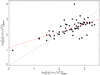 |
Fig. 2 Comparison between spectroscopic and photometric log g. The 1:1 relationship is shown by the black dashed line. A systematic trend is illustrated by the red dashed line. The final photometric log g values were corrected for this trend. |
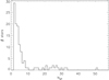 |
Fig. 3 Distribution of the number of effective observations per target for our final sample of 114 targets with 826 effective observationsdescribed in Sect. 2.2. |
2.5 Photometric log(g) estimations
We estimated photometric log g values froma grid of isochrones of solar metallicity by using the CMD6 Web Interface (e.g., Bressan et al. 2012; Tang et al. 2014; Chen et al. 2014, 2015). Each isochrone was traced on a grid  by using linear interpolation and the empty spaces between the isochrones were fulfilled by evolving a Laplace interpolation. This single grid was used for the sake of simplicity, considering that the clusters have a metallicity around the solar value. The central location of each target in the grid was used to get the theoretical log g value, which was set as an initial photometric log g estimation for the target.
After estimating an initial log g for all the targets, we plotted these values against the corresponding measured spectroscopic values and verified a systematic linear trend between them (see Fig. 2). We then corrected this trend to obtain the final photometric log g estimations.The standard deviation between the photometric and spectroscopic log g values is ~0.5 dex. Thus, it waspossible to use these photometric estimations with caution for the purpose of our work – the analysis of log g versus ΔRV∕2 described in Sect. 3.2.
2.6 Number of observations and time series analysis
We defined an arbitrary threshold of at least nine effective observations to perform time-series analysis of our planet-host and binary candidates. This is roughly a minimal requirement to obtain an orbital solution without ambiguity. Figure 3 shows the distribution of effective observations for the stars of our sample. There are 94 stars with less than nine observations and 20 stars with at least nine observations. The time-series analyses are presented in Sects. 3.3 and 3.4 for the best planet-host candidates and for a binary candidate. An overall discussion of all the planet-host candidates is presented in Sect. 3.5.
3 Results
Our final sample of 114 targets, obtained as described in Sect. 2.2, is listed in Table A.1. The table includes the apparent visual magnitude (Vmag), stellar surface gravity (log g), and CORAVEL RV measurements (RVM08) from Mermilliod et al. (2008). Our data are the effective number of observations (Neff), time span (tspan), the RV average ( ), the half peak-to-peak RV (ΔRV∕2), and the difference between the HARPS and CORAVEL RV values with respect to their offsets (ΔRVH−C), these computed for each target. There is also a flag indicating the binary and planet-host candidates. The flag definitions and more details about the table parameters are discussed below.
3.1 Binary candidates
Even if we avoided spectroscopic binaries in our sample (based on data from the literature), binarity can still be present. We used our HARPS observations as well as a comparison with the CORAVEL data to identify potential new binaries.
The maximum ΔRV∕2 value induced by a planet can be estimated by considering a 15 MJ companion in a circular 30-day period orbit (i.e., located approximately at the Roche lobe limit) around a star of 2.0 M⊙ (minimum stellar mass of our sample). Such a system produces an orbital stellar semiamplitude K of ~0.6 km s−1, and so any targets with semiamplitude higher than this should be associated with binary candidates. There is one star that shows a high ΔRV∕2 of 764 m s−1 in our HARPS data. We then included this star, NGC 5822 201, in the list of binary candidates, flagged in Table A.1 as “[B]”, and it is analyzed in detail in Sect. 3.4. Apart from NGC 5822 201, the highest ΔRV∕2 in our HARPS data is 198 m s−1, so we have no indications of other binaries within the HARPS time series. However, long-period binaries can be identified from a comparison between HARPS and CORAVEL. The minimum gap between the CORAVEL (from year 1978 to 1997) and HARPS (from 2005 to 2015) observations is 7 yr.
Figure 4 shows the distribution of the difference between the HARPS and CORAVEL RV data,  , computed by taking the average RV from each instrument. This distribution can be well-fitted with a Gaussian, from which we derive the global offset between these two instruments (the Gaussian center of 131 m s−1, with a σ of 129 m s−1). The binary stars likely lie out from the peak of this distribution. However, RV in each cluster may depend on several factors, which include stellar effective temperature, gravity, metallicity, and other systematic effects. We therefore opted for a more refined selection criteria by computing the offset between the two instruments for each cluster, instead of using the overall distribution of Fig. 4, for the selection of the binary candidates. This offset was estimated by taking the median of
  when having three or more stars, or the smallest variation of
 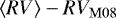 when having only two stars. Stars that deviate from the cluster offset by more than 0.7 km s−1 are considered as binary candidates. The value of 0.7 km s−1 represents the 5σ distribution of Fig. 4. A conservative choice is justified by the consideration that such a deviation shall account also for stellar intrinsic RV variability and uncertainties in the CORAVEL measurements (typically 0.3 km s−1 per CORAVEL observation). In addition, 0.7 km s−1 is larger than the signal expected by a planet, as computed above. From Fig. 4, it is clear that at least eight stars have RV differences above 1.0 km s−1.
Using the above methodology, 13 additional binary candidates were identified, flagged as “B” in Table A.1. These binaries were observed with HARPS only for the years 2013–2015, explaining the reason why their variability was not detected from the HARPS data alone. The total of 14 binaries (“B” and “[B]” flags) were then removed from our sample to obtain a subsample of 101 likely single stars. This subsample is considered in the following section, which is dedicated to the identification of planet-host candidates.
Table 2 summarizes the selection of the single-star candidates, based on the CORAVEL versus HARPS analysis described above. The number of targets for each cluster (Ni), the corresponding number of single starcandidates (Nf), the instrumental RV offset (Offset), and the RV standard deviation (σ) are provided. The Offset and σ values were computed in two steps, before and after the removal of the binaries, and the table shows the final values. The typical offset for each cluster lies around 100–300 m s−1, which is compatible with the global offset illustrated in Fig 4. An atypical case is that of NGC 2345 with an offset of − 529 m s−1, which deviates strongly from the other clusters. We cannot confidently explain the reason for this deviation.
 |
Fig. 4 Distribution of the difference between the RV average obtained with HARPS and the RV average obtained with CORAVEL for each target. The range is truncated for a better display; the whole distribution ranges from − 5.86 to 4.16 km s−1. A Gaussian fit is shown with its center and 5σ range. |
Summary of the selection of single star candidates for each cluster.
3.2 Planet-host candidates
After the removal of the binaries, our subsample of likely single stars comprises 769 observations of 101 targets. Most targets have a small number of observations and cannot be used for a proper time-series analysis and orbit determination. We therefore selected the best planet-host candidates based on the work of Hekker et al. (2008), as explained in Sect. 2.4, with the basic criterion defined by Eqs. (25)–(27) of Troup et al. (2016).
Equation (25) of Troup et al. (2016) can be represented in log–log scale by
![Mathematical equation: \begin{equation*} \log(\UpDelta RV_{\rm{trend}}/2 {\rm{~[km\,s^{-1}]~}}) = a + b\log g, \end{equation*}](/articles/aa/full_html/2018/12/aa33123-18/aa33123-18-eq8.png) (2)
(2)
where the parameters a = log2 and 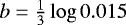 reproduce the trend of Hekker et al. (2008). This trend was estimated using targets with typically 20–100 observations, which provide more reliable ΔRV∕2 measurements than for our sample. Most of our objects have a low number of observations and this may bias the level of ΔRVtrend∕2. Hence, we computed a fit to our sample by fixing the slope b at the value found in Troup et al. (2016) and leaving a as a free parameter. For the fit, we considered only the 64 objects with spectroscopic log g (see Sect 2.4). The best fit was obtained with a = −0.172 dex.
Figure 5 depicts ΔRV∕2 versus log g for our subsample of 101 single star candidates. The intrinsic variability (stellar jitter) trend is illustrated by the black solid line, the 3× level is given by the black dotted line, and the 3× typical RV error is depicted by the gray dashed line. There are 11 stars lying above both the 3× trend level and the 3× typical RV error, which are the best planet-host candidates. The candidates with at least nine observations – namely those chosen to be analyzed in more detail from their time series (see Sect. 2.6) – are labeled A–D. Some stars may rise above the threshold and become planet-host candidates when having more observations.
Table 3 provides an overview of the planet and binary candidates for all the open clusters in our program sorted by their turnoff masses MTO. These were estimated from CMD7 Web Interface isochrones corresponding to the age and metallicity of each cluster. The parameters log (t), [Fe∕H], e(B−V), and μ stand for their age, metallicity, reddening, and distance modulus, respectively. The table also contains N*, Np , and Nb , which are the number of stars belonging to each cluster of our final sample described in Sect. 2.2, the number of planet-host candidates identified in this work, and the number of binary candidates, respectively. Four out of the 29 open clusters observed still have no targets containing at least two effective observations.
The number of observations in our sample is still very limited to provide a proper census of planet hosts in young open clusters. For now, two clusters, IC 4756 and IC 2714, have three planet-host candidates each. This could indicate a high planet occurrence rate for these clusters or the planet-host candidates may be false positives. These two clusters lie in a relatively narrow MTO range around ~2.5–3.1 M⊙, whereas the clusters outside this range have either zero or one candidate. The larger number of candidates within this range qualitatively agrees with recent studies which show that the planet occurrence rate as a function of stellar mass has a maximum for giant host stars around ~2 M⊙ (e.g., Reffert et al. 2015). These studies also claim that the occurrence rate drops rapidly for higher masses. Indeed, we have only one candidate among the sample of the 40 most massive stars (MTO > 3.1 M⊙). Such a low incidence of planets in massive stars can be understood within a scenario in which strong winds from high-mass stars may generate competing timescales between disk dissipation and planet formation (e.g., Kennedy & Kenyon 2009; Ribas et al. 2015). However, we note that some observational biases may reduce the planet detectability when increasing the host mass (e.g., Jones et al. 2014). For instance, some of our planet-host candidates would produce orbital semiamplitudes below the 3× trend line of Fig. 5 if they were observed around more massive stars (see Sect. 3.5 for a specific example). In addition, more luminous giants tend to have a larger intrinsic stellar noise, and this also introduces bias.
Overview of planet and binary candidates each cluster.
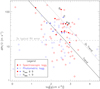 |
Fig. 5 RV half peak-to-peak difference, ΔRV∕2, as a function of log g, for our subsample of 101 single stars. Open circles stand for targets with a number of observations between two and eight, whereas filled circles represent the targets with at least nine observations. Red circles refer to the targets with spectroscopic log g measurements, whereas blue circles illustrate those with photometric measurements. The gray horizontal dashed line represents the 3× RV typicalerror level. The black solid line illustrates the linear fit of the data and the black dotted line is its 3× level. The planet-host candidates lie in the upper right region encompassed within the dashed and the dotted lines. The candidates with at least nine observations are labeled A to D. The red cross illustrates the residual for target D (IC 4651 9122) after removing the planet signal. |
3.3 Long-term variations in IC 2714 stars
Targets labeled A, B, and C in Fig. 5 have at least nine observations and lie above the 3× level of the log g versus RV trend. Hence, these are good planet-host candidates and, theoretically, they have enough data for a time series analysis. We analyzed generalized Lomb-Scargle (GLS) periodograms (Zechmeister & Kürster 2009) for these RV time series to look for orbit-related signals. The periodograms provide periods with false alarm probability (FAP) less than 1%, but Keplerian fits to the data provide doubtful or ambiguous solutions.
These targets all belong to the same cluster, IC 2714, and their RV time series show linear trends of a few (5–10) m s−1 yr−1, as shown in Fig 6. No pulsation or rotational modulation with such a long period is expected in the evolutionary stage of these stars (between the RGB-base and the red clump; e.g., Delgado Mena et al. 2016). Our S index measurements also do not showany conclusive correlation, so longer time span observations are needed to verify the origin of the RV variation, including the possibility of a substellar companion.
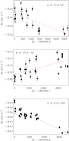 |
Fig. 6 RV time series of the targets labeled A, B, and C in Fig. 5. All stars belong to the cluster IC 2714 and their RV data exhibit long-term RV variations, illustrated by the red dashed lines. |
3.4 Orbital solutions for IC 4651 9122b and NGC 5822 201B
The star labeled D, IC 4651 9122, has a very clear RV periodic variation. Figure 7 shows a set of standard analyses performed for this star. The GLS periodogram (top panel) shows a strong peak with a FAP < 10−9 corresponding to a peak of about 2 yr. A Keplerian model fits well with the observed data, as shown in the middle and bottom panels, suggesting the presence of a planet, namely IC 4651 9122b.
From Fig. 5, the star is expected to have an intrinsic variability (jitter) of ~20 ms−1. To be conservative, an upper limit for this jitter is of ~60 m s−1, namely the 3× trend. We used the RVLIN and BOOTTRAN codes8 (Wright & Howard 2009; Wang et al. 2012) to calculate the orbital parameters by testing different jitter levels from 10 to 60 m s−1. In a first test, we performed a Monte Carlo approach by computing independent Keplerian fits with random fluctuations to the RV data within a certain jitter level added in quadrature to the RV errors. For verification, we used the bootstrapping method from the BOOTTRAN code. The solutions were rather stable for or all the tests, including for an upper jitter level of 60 m s−1. The orbital parameters obtained from our Monte Carlo approach for the most likely stellar jitter level of 20 m s−1 are given in Table 4.
Although the RV periodic variation in Fig. 7 is obvious, we used the S index and the bisector span to establish the nature of the RV periodicity. It was necessary to consider a data subset with high S/N for the S index because this parameter is not reliable at low S/N. Figure 8 shows a systematic increase of the S index with decreasing S/N, which occurs because the CaII H & K lines become dominated by noise. The bisector also loses confidence at low S/N. Hence, we split the data into lower and higher S/N regimes, namely S∕N < 21 and S∕N ≥ 21 (at 400 nm), for a proper interpretation of our results. These regimes are illustrated in our analysis by the gray and black circles, respectively.
Figure 9 displays the activity proxy tests. The GLS periodograms (left panels) show no confident period related with the orbit of the planet, and the RV versus activity proxy diagrams (right panels) have low correlations. A small subset of data where the S index seems to increase with increasing RV (gray circles in the top right panel) is not to be trusted, as the S/N of the data is too low. Overall, this analysis shows no association between the activity proxies and RV, thus supporting the orbital origin for the main RV variation.
We also analyzed the residual of the observed RV data after removing the best Keplerian fit for IC 4651 9122, as shown in Fig 10. There is a signal which is still noticeable after subtraction whose nature is yet to be determined. The GLS periodogram provides a prominent peak period of about 1 yr, which is half of the 2-yr period of IC 4651 9122b. However, systematic effects, such as 1-yr seasonal variation, may contribute to this period, which does not survive when removing some data points at random. The ΔRV∕2 level of this residual (see Fig. 5) lies below the region we defined for planet-host candidates, so this signal may not be caused by a second planet. The S index in Fig. 10 (top right panel) does not exclude the possibility of a second planet, since it shows no significant correlation with RV.
Finally, we analyzed the time series of NGC 5822 201, identified in Sect. 3.1 as a binary candidate. Figure 11 shows the periodogram of the RV time series in the top panel and the RV time series in the bottom panel. The orbital nature of this signal is very clear and the best Keplerian fit parameters computed from our Monte Carlo approach are given in Table 5. For proper error calculations, we assumed a jitter of 45 m s−1 for the primary starbased on its log g value of 2.85 ± 0.08 dex and on the trend curve of Fig. 5.
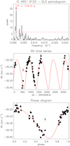 |
Fig. 7 RV analysis of IC 4651 9122. Top panel: GLS periodogram of the RV time series showing the most prominent peak period. The red horizontal dashed line illustrates the 1% FAP level. Middle panel: RVtime series, where the black circles and error bars are the HARPS data and the red curve is the best Keplerian fit to the data. The gray colored data point is a particular outlier with a S∕N = 10.3, namely very close to the threshold (S∕N = 10.0) defined in this work. We discarded it in this analysis. Bottom panel: phase diagram of the RV time series for the orbital period of the best fit (see Table 4). The symbols are as in the middle panel. |
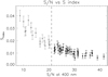 |
Fig. 8 S index vs. S/N at 400 nm for the HARPS observations of IC 4651 9122. For S∕N < 21, the S index shows a strong trend with S/N that is not reliable. |
Orbital parameters for the new giant planet IC 4651 9122b.
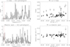 |
Fig. 9 Analysis of activity proxies for IC 4651 9122. Left panels: GLS periodograms of the S index and of the bisector span time series by considering the data subset with S∕N ≥ 21. The red vertical dashed line illustrates the orbital period of the Keplerian fit described in Table 4. Right panels: correlation between RV and each activity proxy, where the data are split into S∕N < 21 (gray circles) and S∕N ≥ 21 (black circles). The Pearson correlation coefficient is 0.20 for RV versus S index and 0.15 for RV versus bisector span when considering the data subset with S∕N ≥ 21. |
Orbital parameters for the binary companion NGC 5822 201B.
3.5 Possible orbital parameters for the planet candidates
In this section, we provide an overall discussion of the planet-host candidates by considering possible orbital solutions in case the planets were confirmed. The minimum planet mass, m sini, is computedfrom the RV equation, where the stellar mass and the RV semiamplitude are assumed to be M* ≃ MTO and K ≃ ΔRV∕2, respectively. The orbital period P and eccentricity e are unknown for any planet candidate (except for the confirmed planet IC 4651 9122b). We thus have assumed a low eccentricity (≲0.3) for possible planets, whereas, as far as orbital periods are concerned, a more detailed discussion is required. That discussion is presented below, being mostly based on a visual inspection of the RV time series with a limited number of observations.
Rough orbital parameters can be suggested for the IC 2714 planet-host candidates based on Fig. 6 from Sect 3.3. In general, the long-term RV variations of these candidates would fulfill at most half a cycle of hypothetical orbits for all cases. Orbital periods should therefore be as long as at least twice the total time span (of ~3200–3700 days) of the HARPS observations. From this assumption, hypothetical planets would lie more than ~10 AU away from their host stars and would have masses greater than ~10 MJ. These candidates are good examples for illustrating the detectability bias mentioned in Sect. 3.2: they would produce RV semiamplitudes about 30% smaller, thus below the 3× trend line of Fig. 5, if they were observed around a 6 M⊙ star.
Limited observations of the remaining candidates show, except for the most massive one (NGC 2925 108, with 5.9 M⊙), noticeable RV variations likely within short time spans. Such a signature is compatible either with possible presence of close-in planets with a few Jupiter masses or with intrinsic stellar signal. The most massive candidate has six observations spread over a ~700 days time span showing likely a long-term variation similar to the IC 2714 candidates, thus indicating presence of a possible long-period and massive planet.
Overall, an interesting aspect is the close similarity between the RV variations of the planet-host candidates in IC 2714. If these variations were due to planetary companions, their preliminary orbital parameters would indicate presence of rather massive planets around massive stars. Such a trend qualitatively agrees with a commonly proposed scenario where more massive stars would be formed with correspondingly more massive protoplanetary disks that would yield more massive planets (e.g., Ida & Lin 2005; Kennedy & Kenyon 2008). Finally, the NGC 2925 108 candidate is another interesting case because, if confirmed, it may extend planet detection in open clusters over a broader stellar mass range where a low planet incidence has been observed (see Sect. 3.2).
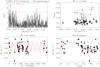 |
Fig. 10 RV and activity proxy analyses for the residual of the RV time series of IC 4651 9122 after removing the best Keplerian fit. The GLS periodogram (top left panel), the RV versus S index correlation (top right panel), theRV time series (bottom left panel), and the RV phase diagram (bottom right panel) follow similar definitions to those described in Figs. 7 and 9. The Pearson correlation coefficient is 0.27 forRV versus S index and 0.15 for RV versus bisector span when considering the data subset with S∕N ≥ 21. |
4 Conclusions
We present the first results of a long-term survey where we look for massive exoplanets orbiting intermediate-mass (~2–6 M⊙) giant stars belonging to 29 open clusters. This survey aims to provide in the future, following the collection of more data, a census of a diversity of stellar and planetary environments with detailed physical descriptions. These will include stellar absolute physical parameters and planetary orbital solutions, based on a homogeneous set of HARPS observations.
We identify 14 new binary candidates, by combining our observations with CORAVEL data, spanning a ~30 yr (from 1978 to 2015) baseline, despite sample pre-selection aimed to avoid binaries. We then considered 101 single stars, among which we detected 11 planet-host candidates. It is worth noting that 10 of the 11 candidates have masses ≲ 3.2 M⊙, and only 1 candidate has mass greater than this. This agrees qualitatively with recent studies concerning the occurrence rate of massive planets as a function of the host star masses, which shows, for the case of giant stars, a peak around ~2 M⊙ and a low rate for higher masses (e.g., Reffert et al. 2015). We do, however, warn the reader that our selection method has an intrinsic bias against more massive stars.
Three of the planet-host candidates belong to the same cluster, IC 2714, and show common behavior, which is long-term RV variation that cannot be resolved with the current observations. More observations are needed to verify whether they are induced by substellar companions. One planet-host candidate, IC 4651 9122, shows very clear RV periodic variation. Time series analysis and tests of activity proxies confirmed this star has a giant planet companion, namely IC 4651 9122b, with a minimum mass of 6.3 MJ and a semimajor axis of 2.0 AU. There is a residual signal that may have a physical origin, but it also requires more observations for proper interpretation. Finally, we also have enough data for one of the binary candidates, NGC 5822 201, to study it in further detail. The companion, NGC 5822 201B, has a very low minimum mass of 0.11 M⊙ and a semimajor axis of 6.5 AU, which is comparable to the Jupiter distance to the Sun.
The number of known sub-stellar objects around giants is still rather small. Brown dwarfs orbiting Sun-like stars seem to become less frequent when the mass of the star increases, whereas planets become more frequent (e.g., Grether & Lineweaver 2006). This behavior may be different for more massive or giant stars, as suggested in some studies (e.g., Lovis & Mayor 2007) and indicated qualitatively in Sect. 3.2. Overall, our small sample of planet-host candidates can extend this study to more massive stars in relation to previous works. It indicates a possible dependence of the planet incidence upon the stellar mass, as well as some relation between host star mass and planetary mass, that are qualitatively compatible with theoretical and observational studies. Observing more giant stars in clusters may therefore provide essential information to better understand these distributions as well as other aspects.
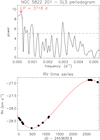 |
Fig. 11 RV time series analysis for NGC 5822 201. Top panel: GLS periodogram. Bottom panel: RV time series. Symbols follow the same definitions as in Fig. 7. |
Acknowledgements
Research activities of the Observational Astronomy Board of the Federal University of Rio Grande do Norte (UFRN) are supported by continuous grants from the CNPq and FAPERN Brazilian agencies. I.C.L acknowledges a Post-Doctoral fellowship at the European Southern Observatory (ESO) supported by the CNPq Brazilian agency (Science Without Borders program, Grant No. 207393/2014-1). B.L.C.M. acknowledges a PDE fellowship from CAPES. S.A. acknowledges a Post-Doctoral fellowship from the CAPES Brazilian agency (PNPD/2011: Concessão Institucional), hosted at UFRN from March 2012 to June 2014. G.P.O. acknowledges a graduate fellowship from CAPES. Financial support for C.C. is provided by Proyecto FONDECYT Iniciación a la Investigacion 11150768 and the Chilean Ministry for the Economy, Development, and Tourism’s Programa Iniciativa Científica Milenio through grant IC120009, awarded to Millenium Astrophysics Institute. D.B.F. acknowledges financial support from CNPq (Grant No. 306007/2015-0). L.P. acknowledges a distinguished visitor PVE/CNPq appointment at the Physics Graduate Program of UFRN in Brazil and thanks to DFTE/UFRN for hospitality. We also acknowledge the Brazilian institute INCT INEspaço for partial financial support. Finally, we warmly thank the anonymous referee for very constructive comments.
Appendix A Additional table
References
- Baliunas, S. L., Donahue, R. A., Soon, W. H., et al. 1995, ApJ 438, 269 [NASA ADS] [CrossRef] [Google Scholar]
- Barros, S. C. C., Demangeon, O., & Deleuil, M. 2016, A&A, 594, A100 [NASA ADS] [CrossRef] [EDP Sciences] [Google Scholar]
- Baumgardt H., Dettbarn C., & Wielen R. 2000, A&AS, 146, 251 [NASA ADS] [CrossRef] [EDP Sciences] [Google Scholar]
- Bressan, A., Marigo, P., Girardi, L., et al. 2012, MNRAS, 427, 127 [NASA ADS] [CrossRef] [Google Scholar]
- Brucalassi, A., Koppenhoefer, J., Saglia, R., et al. 2017, A&A, 603, A85 [NASA ADS] [CrossRef] [EDP Sciences] [Google Scholar]
- Brucalassi, A., Pasquini, L., Saglia, R., et al. 2014, A&A, 561, L9 [NASA ADS] [CrossRef] [EDP Sciences] [Google Scholar]
- Brucalassi, A., Pasquini, L., Saglia, R., et al. 2016, A&A, 592, L1 [NASA ADS] [CrossRef] [EDP Sciences] [Google Scholar]
- Chen, Y., Girardi, L., Bressan, A., et al. 2014, MNRAS, 444, 2525 [NASA ADS] [CrossRef] [Google Scholar]
- Chen, Y., Bressan, A., Girardi, L. 2015, MNRAS, 452, 1068 [NASA ADS] [CrossRef] [Google Scholar]
- Curtis, J. L., Vanderburg, A., Torres, G., et al. 2018, AJ, 155, 173 [NASA ADS] [CrossRef] [Google Scholar]
- David, T. J., Conroy, K. E., Hillenbrand, L. A., et al. 2016, AJ, 151, 112 [NASA ADS] [CrossRef] [Google Scholar]
- Delgado Mena, E., Tsantaki, M., Sousa, S. G., et al. 2016, A&A 587, A66 [NASA ADS] [CrossRef] [EDP Sciences] [Google Scholar]
- Frinchaboy, P.M., & Majewski, S. R. 2008, AJ, 136, 118 [NASA ADS] [CrossRef] [Google Scholar]
- Gonzalez, G. 1997, MNRAS, 285, 403 [NASA ADS] [CrossRef] [Google Scholar]
- Grether, D., & Lineweaver, C. H. 2006, ApJ, 640, 1051 [NASA ADS] [CrossRef] [Google Scholar]
- Haywood, M. 2009, ApJ, 698, L1 [NASA ADS] [CrossRef] [Google Scholar]
- Heiter, U., Soubiran, C., Netopil, M., et al. 2014, A&A, 561, A93 [NASA ADS] [CrossRef] [EDP Sciences] [Google Scholar]
- Hekker, S., Reffert, S., Quirrenbach, A., et al. 2006, A&A, 454, 943 [NASA ADS] [CrossRef] [EDP Sciences] [Google Scholar]
- Hekker, S., Snellen, I. A. G., Aerts, C., et al. 2008, A&A, 480, 215 [NASA ADS] [CrossRef] [EDP Sciences] [Google Scholar]
- Ida, S., & Lin, D. N. C. 2005, ApJ, 626, 1045 [NASA ADS] [CrossRef] [Google Scholar]
- Israelian, G., Delgado Mena, E., Santos, N. C., et al. 2009, Nature, 462, 189 [NASA ADS] [CrossRef] [PubMed] [Google Scholar]
- Johnson, J. A., Fischer, D. A., Marcy, G. W., et al. 2007, ApJ, 665, 785 [NASA ADS] [CrossRef] [Google Scholar]
- Jones, M. I., Jenkins, J. S., Bluhm, P., et al. 2014, A&A, 566, A113 [NASA ADS] [CrossRef] [EDP Sciences] [Google Scholar]
- Jones, M. I., Jenkins, J. S., Brahm, R., et al. 2016, A&A, 590, A38 [NASA ADS] [CrossRef] [EDP Sciences] [Google Scholar]
- Kennedy, G. M., & Kenyon, S. J. 2008, ApJ, 673, 502 [NASA ADS] [CrossRef] [Google Scholar]
- Kennedy, G. M., & Kenyon, S. J. 2009, ApJ, 695, 1210 [NASA ADS] [CrossRef] [Google Scholar]
- Kharchenko N. V., Piskunov A. E., Roeser S., et al. 2005, A&A, 438, 1163 [NASA ADS] [CrossRef] [EDP Sciences] [MathSciNet] [Google Scholar]
- Kjeldsen, H., & Bedding, T. R. 1995, A&A, 293, 87 [NASA ADS] [Google Scholar]
- Laughlin, G., & Adams, F. C. 1997, ApJ, 491, L51 [NASA ADS] [CrossRef] [Google Scholar]
- Libralato, M., Nardiello, D., Bedin, L. R., et al. 2016, MNRAS, 463, 1780 [NASA ADS] [CrossRef] [Google Scholar]
- Lovis, C., & Mayor, M. 2007, A&A, 472, 657 [NASA ADS] [CrossRef] [EDP Sciences] [Google Scholar]
- Majewski, S. R., Schiavon, R. P., Frinchaboy, P. M., et al. 2017, AJ, 154, 94 [NASA ADS] [CrossRef] [Google Scholar]
- Malavolta, L., Nascimbeni, V., Piotto, G., et al. 2016, A&A, 588, A118 [NASA ADS] [CrossRef] [EDP Sciences] [Google Scholar]
- Mann, A. W., Gaidos, E., Mace, G. N., et al. 2016, ApJ, 818, 46 [NASA ADS] [CrossRef] [Google Scholar]
- Mann, A. W., Gaidos, E., Vanderburg, A., et al. 2017, AJ, 153, 64 [Google Scholar]
- Mann, A. W., Vanderburg, A., Rizzuto, A. C., et al. 2018, AJ, 155, 4 [NASA ADS] [CrossRef] [Google Scholar]
- Mayor, M., & Queloz, D. 1995, Nature, 378, 355 [NASA ADS] [CrossRef] [Google Scholar]
- Mayor, M., Pepe, F., Queloz, D., et al. 2003, The Messenger, 114, 20 [NASA ADS] [Google Scholar]
- Meibom, S., Torres, G., Fressin, F., et al. 2013, Nature, 499, 55 [NASA ADS] [CrossRef] [Google Scholar]
- Mermilliod, J.-C. 1995, Astrophys. Space Sci. Lib., 203, 127 [Google Scholar]
- Mermilliod, J. C., Mayor, M., & Udry, S. 2008, A&A, 485, 303 [NASA ADS] [CrossRef] [EDP Sciences] [Google Scholar]
- Nardiello, D., Libralato, M., Bedin, L. R., et al. 2016, MNRAS, 463, 1831 [NASA ADS] [CrossRef] [Google Scholar]
- Obermeier, C., Henning, T., Schlieder, J. E., et al. 2016, AJ, 152, 223 [NASA ADS] [CrossRef] [Google Scholar]
- Pasquini, L., Döllinger, M. P., Weiss, A., et al. 2007, A&A, 473, 979 [NASA ADS] [CrossRef] [EDP Sciences] [Google Scholar]
- Pasquini, L., Brucalassi, A., Ruiz, M. T., et al. 2012, A&A, 545, A139 [NASA ADS] [CrossRef] [EDP Sciences] [Google Scholar]
- Pollack, J., Hubickyj, O., Bodenheimer, P., et al. 1996, Icarus, 124, 62 [NASA ADS] [CrossRef] [Google Scholar]
- Pope, B. J. S., Parviainen, H., & Aigrain, S. 2016, MNRAS, 461, 3399 [NASA ADS] [CrossRef] [Google Scholar]
- Queloz, D., Henry, G. W., Sivan, J. P., et al. 2001, A&A, 379, 279 [NASA ADS] [CrossRef] [EDP Sciences] [Google Scholar]
- Quinn, S. N., White, R. J., Latham, D. W., et al. 2012, ApJ, 756, L33 [NASA ADS] [CrossRef] [Google Scholar]
- Quinn, S. N., White, R. J.. Latham, D. W., et al. 2014, ApJ, 787, 27 [NASA ADS] [CrossRef] [Google Scholar]
- Reffert, S., Bergmann, C., Quirrenbach, A., et al. 2015, A&A, 574, A116 [NASA ADS] [CrossRef] [EDP Sciences] [Google Scholar]
- Ribas, A., Bouy, H., & Merín, B. 2015, A&A 576, A52 [NASA ADS] [CrossRef] [EDP Sciences] [Google Scholar]
- Santos, N. C., Mayor, M., Naef, D., et al. 2002, A&A, 392, 215 [NASA ADS] [CrossRef] [EDP Sciences] [Google Scholar]
- Santos, N. C., Israelian, G., & Mayor, M. 2004, A&A, 415, 1153 [NASA ADS] [CrossRef] [EDP Sciences] [Google Scholar]
- Sato, B., Izumiura, H., Toyota, E., et al. 2007, ApJ, 661, 527 [NASA ADS] [CrossRef] [Google Scholar]
- Schröder, C., Reiners, A., & Schmit, J. H. M. M. 2009 A&A 493, 1099 [NASA ADS] [CrossRef] [EDP Sciences] [Google Scholar]
- Setiawan, J., Pasquini, L., da Silva, L., et al. 2004, A&A, 421, 241 [Google Scholar]
- Soubiran, C., Le Campion, J.-F., Cayrel de Strobel, G., et al. 2010, A&A, 515, A111 [NASA ADS] [CrossRef] [EDP Sciences] [Google Scholar]
- Soubiran, C., Le Campion, J.-F., Brouillet, N., et al. 2016, A&A, 591, A118 [NASA ADS] [CrossRef] [EDP Sciences] [Google Scholar]
- Tang, J., Bressan, A., Rosenfield, P. 2014, MNRAS, 445, 4287 [NASA ADS] [CrossRef] [Google Scholar]
- Troup, N. W., Nidever, D. L., De Lee, N., et al. 2016, AJ, 151, 85 [NASA ADS] [CrossRef] [Google Scholar]
- Wang, Sharon, X., Wright, J. T., Cochran, W., et al. 2012, ApJ, 761, 46 [NASA ADS] [CrossRef] [Google Scholar]
- Wright, J. T., & Howard, A. W. 2009, ApJS, 182, 205 [ERRATUM: 2013, ApJS, 205, 22] [NASA ADS] [CrossRef] [Google Scholar]
- Wu, Z.-Y., Zhou, X., Ma, J., et al. 2009, MNRAS, 399, 2146 [NASA ADS] [CrossRef] [Google Scholar]
- Zechmeister, M., & Kürster, M. 2009, A&A 496, 577 [NASA ADS] [CrossRef] [EDP Sciences] [Google Scholar]
All Tables
Number of observed stars (Nobj) of our original list of 29 open clusters and total number of HARPS observations (Nobs) carried out by our and other programs for each cluster.
All Figures
|
Fig. 1 Photon noise error in the measurement of the CCF center of single observations vs. S/N at 490 nm for our sample of open cluster targets observed with HARPS. The overall RV errors are typically distributed around 1–4 m s−1 and range from 42 cm s−1 to 119 m s−1. The overall S/N distribution peaks around 20–40 and ranges from 2.4 to 223. Black filled circles are the selected data, and gray crosses are the discarded ones, all identified from a visual inspection of the CCFs. Black open circles depict the data with S∕N < 10 that were also discarded and this threshold is represented by the vertical dashed line. |
| In the text | |
|
Fig. 2 Comparison between spectroscopic and photometric log g. The 1:1 relationship is shown by the black dashed line. A systematic trend is illustrated by the red dashed line. The final photometric log g values were corrected for this trend. |
| In the text | |
|
Fig. 3 Distribution of the number of effective observations per target for our final sample of 114 targets with 826 effective observationsdescribed in Sect. 2.2. |
| In the text | |
|
Fig. 4 Distribution of the difference between the RV average obtained with HARPS and the RV average obtained with CORAVEL for each target. The range is truncated for a better display; the whole distribution ranges from − 5.86 to 4.16 km s−1. A Gaussian fit is shown with its center and 5σ range. |
| In the text | |
|
Fig. 5 RV half peak-to-peak difference, ΔRV∕2, as a function of log g, for our subsample of 101 single stars. Open circles stand for targets with a number of observations between two and eight, whereas filled circles represent the targets with at least nine observations. Red circles refer to the targets with spectroscopic log g measurements, whereas blue circles illustrate those with photometric measurements. The gray horizontal dashed line represents the 3× RV typicalerror level. The black solid line illustrates the linear fit of the data and the black dotted line is its 3× level. The planet-host candidates lie in the upper right region encompassed within the dashed and the dotted lines. The candidates with at least nine observations are labeled A to D. The red cross illustrates the residual for target D (IC 4651 9122) after removing the planet signal. |
| In the text | |
|
Fig. 6 RV time series of the targets labeled A, B, and C in Fig. 5. All stars belong to the cluster IC 2714 and their RV data exhibit long-term RV variations, illustrated by the red dashed lines. |
| In the text | |
|
Fig. 7 RV analysis of IC 4651 9122. Top panel: GLS periodogram of the RV time series showing the most prominent peak period. The red horizontal dashed line illustrates the 1% FAP level. Middle panel: RVtime series, where the black circles and error bars are the HARPS data and the red curve is the best Keplerian fit to the data. The gray colored data point is a particular outlier with a S∕N = 10.3, namely very close to the threshold (S∕N = 10.0) defined in this work. We discarded it in this analysis. Bottom panel: phase diagram of the RV time series for the orbital period of the best fit (see Table 4). The symbols are as in the middle panel. |
| In the text | |
|
Fig. 8 S index vs. S/N at 400 nm for the HARPS observations of IC 4651 9122. For S∕N < 21, the S index shows a strong trend with S/N that is not reliable. |
| In the text | |
|
Fig. 9 Analysis of activity proxies for IC 4651 9122. Left panels: GLS periodograms of the S index and of the bisector span time series by considering the data subset with S∕N ≥ 21. The red vertical dashed line illustrates the orbital period of the Keplerian fit described in Table 4. Right panels: correlation between RV and each activity proxy, where the data are split into S∕N < 21 (gray circles) and S∕N ≥ 21 (black circles). The Pearson correlation coefficient is 0.20 for RV versus S index and 0.15 for RV versus bisector span when considering the data subset with S∕N ≥ 21. |
| In the text | |
|
Fig. 10 RV and activity proxy analyses for the residual of the RV time series of IC 4651 9122 after removing the best Keplerian fit. The GLS periodogram (top left panel), the RV versus S index correlation (top right panel), theRV time series (bottom left panel), and the RV phase diagram (bottom right panel) follow similar definitions to those described in Figs. 7 and 9. The Pearson correlation coefficient is 0.27 forRV versus S index and 0.15 for RV versus bisector span when considering the data subset with S∕N ≥ 21. |
| In the text | |
|
Fig. 11 RV time series analysis for NGC 5822 201. Top panel: GLS periodogram. Bottom panel: RV time series. Symbols follow the same definitions as in Fig. 7. |
| In the text | |
Current usage metrics show cumulative count of Article Views (full-text article views including HTML views, PDF and ePub downloads, according to the available data) and Abstracts Views on Vision4Press platform.
Data correspond to usage on the plateform after 2015. The current usage metrics is available 48-96 hours after online publication and is updated daily on week days.
Initial download of the metrics may take a while.