| Issue |
A&A
Volume 620, December 2018
The XXL Survey: second series
|
|
|---|---|---|
| Article Number | A15 | |
| Number of page(s) | 16 | |
| Section | Cosmology (including clusters of galaxies) | |
| DOI | https://doi.org/10.1051/0004-6361/201732507 | |
| Published online | 20 November 2018 | |
The XXL Survey
XXX. Characterisation of the XLSSsC N01 supercluster and analysis of the galaxy stellar populations
1
INAF – Osservatorio astronomico di Padova,
Vicolo Osservatorio 5,
35122
Padova,
Italy
e-mail: This email address is being protected from spambots. You need JavaScript enabled to view it.
2
Aix Marseille Univ., CNRS, CNES, LAM,
Marseille,
France
3
Max-Planck-Institut für Extraterrestrische Physik,
Giessenbachstrasse,
85748
Garching,
Germany
4
School of Physics, University of Melbourne, VIC
3010,
Australia
5
Instituto de Radioastronomìa y Astrofìsica, UNAM, Campus Morelia,
A.P. 3-72, C.P.
58089,
Mexico
6
INAF – Istituto di Astrofisica Spaziale e Fisica Cosmica Milano,
Via Bassini 15,
20133
Milan,
Italy
7
Departamento de Astronomìa, DCNE-CGT, Universidad de Guanajuato; Callejón de Jalisco, S/N, Col. Valenciana,
36240
Guanajuato,
Gto.,
Mexico
8
AIM, CEA, CNRS, Université Paris-Saclay, Université Paris Diderot, Sorbonne Paris Cité,
91191
Gif-sur-Yvette,
France
9
INAF – Osservatorio Astronomico di Bologna,
via Gobetti 93/3,
40129
Bologna,
Italy
10
Argelander Institut für Astronomie, Universität Bonn,
Auf dem Huegel 71,
53121
Bonn,
Germany
11
School of Physics, HH Wills Physics Laboratory, Tyndall Avenue,
Bristol
GB-BS8 1TL,
UK
12
Department of Physics and Astronomy, University of Victoria,
3800
Finnerty Road,
Victoria,
BC,
Canada
13
Astrophysics Research Institute, Liverpool John Moores University, IC2,
Liverpool Science Park, 146 Brownlow Hill,
Liverpool
GB-L3 5RF,
UK
14
INAF – Osservatorio Astronomico di Roma,
via Frascati 33,
00078
Monte Porzio Catone (Rome),
Italy
15
School of Physics and Astronomy, Monash University, Clayton,
Victoria
3800,
Australia
16
International Centre for Radio Astronomy Research (ICRAR), The University of Western Australia,
M468, 35 Stirling Highway,
Crawley,
6009,
Australia
17
SUPA, School of Physics & Astronomy, University of St Andrews,
North Haugh,
St Andrews
GB-KY16 9SS,
UK
18
Dipartimento di Fisica e Astronomia, Alma Mater Studiorum - Università di Bologna,
via Gobetti 93/3,
40129
Bologna,
Italy
19
Main Astronomical Observatory, Academy of Sciences of Ukraine,
27 Akademika Zabolotnoho St.,
03680
Kyiv,
Ukraine
20
Department of Physics and Michigan Center for Theoretical Physics, University of Michigan,
Ann Arbor,
MI
48109,
USA
21
ESA/ESTEC,
Noordwijk
2201 AZ,
The Netherlands
22
Astrophysics and Cosmology Research Unit, University of KwaZulu-Natal,
4041
Durban,
South Africa
23
Australian Astronomical Observatory,
PO BOX 915,
North Ryde
1670,
Australia
24
Department of Space, Earth and Environment, Onsala Space Observatory, Chalmers University of Technology,
439 92
Onsala,
Sweden
25
INAF – Osservatorio Astronomico di Brera,
via Brera, 28,
20121
Milano,
Italy
26
Laboratoire Lagrange, UMR 7293, Université de Nice Sophia Antipolis, CNRS, Observatoire de la Côte d’Azur,
06304
Nice,
France
27
Department of Physics and Astronomy, Macquarie University,
NSW 2109, Australia and Australian Astronomical Observatory PO Box 915,
North Ryde NSW
1670,
Australia
28
Department of Astronomy, University of Geneva,
ch. d’Ecogia 16,
1290
Versoix,
Switzerland
29
Physics Department, Aristotle University of Thessaloniki,
54124
Thessaloniki,
Greece
30
IAASARS, National Observatory of Athens,
15236
Penteli,
Greece
31
School of Physics and Astronomy, University of Birmingham, Edgbaston,
Birmingham
GB-B15 2TT,
UK
32
Ulugh Beg Astronomical Institute of Uzbekistan Academy of Science,
33 Astronomicheskaya str.,
Tashkent
100052,
Uzbekistan
33
Department of Physics, University of Zagreb,
Bijenicka cesta 32,
10000
Zagreb,
Croatia
Received:
20
December
2017
Accepted:
18
April
2018
Abstract
Context. Superclusters form from the largest enhancements in the primordial density perturbation field and extend for tens of Mpc, tracing the large-scale structure of the Universe. X-ray detections and systematic characterisations of superclusters and the properties of their galaxies have only been possible in the last few years.
Aims. We characterise XLSSsC N01, a rich supercluster at z ~ 0.3 detected in the XXL Survey, composed of X-ray clusters of different virial masses and X-ray luminosities. As one of the first studies on this topic, we investigate the stellar populations of galaxies in different environments in the supercluster region.
Methods. We study a magnitude-limited (r ≤ 20) and a mass-limited sample (log(M*∕M⊙) ≥ 10.8) of galaxies in the virialised region and in the outskirts of 11 XLSSsC N01 clusters, in high-density field regions, and in the low-density field. We compute the stellar population properties of galaxies using spectral energy distribution (SED) and spectral fitting techniques, and study the dependence of star formation rates (SFR), colours, and stellar ages on environment.
Results. For r ≤ 20, the fraction of star-forming/blue galaxies, computed either from the specific-SFR (sSFR) or rest-frame colour, shows depletion within the cluster virial radii, where the number of galaxies with log (sSFR/ yr−1) > −12 and with (g − r)restframe < 0.6 is lower than in the field. For log(M*∕M⊙) ≥ 10.8, no trends with environment emerge, as massive galaxies are mostly already passive in all environments. No differences among low- and high-density field members and cluster members emerge in the sSFR-mass relation in the mass-complete regime. Finally, the luminosity-weighted age–mass relation of the passive populations within cluster virial radii show signatures of recent environmental quenching.
Conclusions. The study of luminous and massive galaxies in this supercluster shows that while environment has a prominent role in determining the fractions of star-forming/blue galaxies, its effects on the star formation activity in star-forming galaxies are negligible.
Key words: large-scale structure of Universe / X-rays: galaxies: clusters / galaxies: groups: general / galaxies: evolution / galaxies: star formation / galaxies: stellar content
© ESO 2018
1 Introduction
Galaxy stellar population properties, especially star formation history and colour, depend on the environment in which galaxies reside (Spitzer & Baade 1951; Oemler 1974; Davis & Geller 1976; Dressler 1980; Blanton et al. 2005; Ball et al. 2008). On the other hand, the galaxy stellar mass also plays a significant role in determining these properties (Scodeggio et al. 2002; Kauffmann et al. 2003).
Stellar mass and environment have been found to be the main drivers of galaxy transformations in different regimes. Overall, the environment seems to be more relevant for lower mass galaxies, at least as far as quenching is concerned: galaxies in denser environments tend to be redder than galaxies in less dense environments (Haines et al. 2007; Cooper et al. 2010; Pasquali et al. 2010; Peng et al. 2010, 2012; McGee et al. 2011; Sobral et al. 2011; Muzzin et al. 2012; Smith et al. 2012; Wetzel et al. 2012; La Barbera et al. 2014; Lin et al. 2014; Vulcani et al. 2015). By contrast, on average, more massive galaxies have formed their stars and completed their star formation activity at higher redshift than less massive galaxies (known as the downsizing effect; Cowie et al. 1996; Gavazzi et al. 2006; De Lucia et al. 2007; Sánchez-Blázquez et al. 2009), regardless of environment.
While different methods of estimating stellar masses agree reasonably well within the errors (e.g. Bell & de Jong 2001; Bolzonella et al. 2010), different definitions of environment do not always probe the same scales (e.g. Muldrew et al. 2012; Fossati et al. 2015). It is possible to discuss environmental effects in either the global or local context. Concerning the global environment, galaxies are commonly subdivided into superclusters, clusters, groups, and field and void populations. These roughly correspond to halos of different mass. The local environment is generally described using estimates of projected local density, which can be calculated following several definitions and methods (e.g. Kovač et al. 2010; Cucciati et al. 2010; Muldrew et al. 2012; Vulcani et al. 2012; Darvish et al. 2015; Fasano et al. 2015).
Considering the local density, in the local Universe, Baldry et al. (2006) found that the fraction of galaxies in the red sequence is higher in denser environments at any stellar mass in the range 9.0 < log(M*∕M⊙) < 11.0. Similar results have been confirmed at higher redshift (e.g. Scoville et al. 2007; Cucciati et al. 2010, 2017), where many studies show that all features of the global correlation between galaxy colour and environment measured at z ~ 0 (known as galaxy bimodality) are already in place at z ~ 1, with blue galaxies on average occupying regions of lower density than red galaxies (e.g. Wilman et al. 2005; Cucciati et al. 2006; Cooper et al. 2006, 2010; Coil et al. 2008). At these redshifts, the inverse of the specific star formation rate (sSFR), i.e. the time for a galaxy to double its stellar mass, is higher in denser environments (Scoville et al. 2013). Both in the local Universe and at higher redshift, the stellar mass distribution is also sensitive to the local environment, in the sense that more massive galaxies are preferentially found at higher densities (e.g. Hogg et al. 2003; Kauffmann et al. 2004; Blanton et al. 2005; Bolzonella et al. 2010; Cucciati et al. 2010; Vulcani et al. 2012; Davidzon et al. 2016).
In contrast to these studies, Scodeggio et al. (2009) showed that while there is evidence for a colour–density relation at fixed luminosity at z ~ 1, at intermediate redshifts and fixed stellar mass no colour–density relation can be found. At similar redshifts, Tasca et al. (2009) did not find anyvariation in galaxy morphology (i.e. early- versus late-type) as a function of local galaxy density for log (M*∕M⊙) > 10.5. These works both concluded that the properties (colour and morphology) of massive galaxies are independent of environment.
With regard to the global environment, star formation quenching seems to be stronger in clusters, which display higher fractions of red early-type and lower fractions of blue late-type galaxies than the field (e.g. Dressler 1980; Poggianti et al. 1999; Bai et al. 2009; Vulcani et al. 2013), suggesting that clusters are extremely effective in cutting off the galaxy’s ability to form stars. In an evolutionary scenario, Poggianti et al. (2006) and Iovino et al. (2010), showed that galaxy clusters and groups have seen an evolution in their star-forming galaxy fractions that is stronger than in the field, and that the evolution from blue star-forming to red passive types is faster in dense environments and massive halos. This scenario implies that the fraction of red passive galaxies in clusters increases earlier than in the field, supporting again the environmental quenching.
Focusing on the star-forming population, no consensus regarding the properties of active galaxies in the cluster population relative to those in the field has been reached. Some studies have suggested that the difference in the star formation activity between the field and clusters is primarily driven by the relative red fraction instead of the properties of the star-forming population (Muzzin et al. 2012; Koyama et al. 2013; Lin et al. 2014; Jian et al. 2018). For example, Lin et al. (2014) and Jian et al. (2018) have found that the sSFRs of star-forming galaxies in clusters are only moderately lower than those in the field (<0.2–0.3 dex) and that the difference becomes insignificant at group scale. In contrast, other works (e.g. Patel et al. 2009; Vulcani et al. 2010 at intermediate redshift and Haines et al. 2015; Paccagnella et al. 2016 at low-redshift) identified the presence of a population with reduced star formation rate in clusters with respect to the field, suggesting that both the relative numbers of blue star-forming and red passive galaxies and the characteristics of the star-forming population change with environment.
Regarding the global environment, in addition to studies relating the cluster and field populations, there is an increasing focus on even larger structures, superclusters. Superclusters are defined as the most extended density enhancements formed from primordial perturbations on scales of about 100 h−1 Mpc (H0 = 100 h km s−1 Mpc−1; Bahcall& Soneira 1984), and presenting a variety of characterising properties such as morphology, luminosity, and richness (Einasto et al. 2011a,b).
Studying the properties of superclusters helps us to understand the formation, evolution, and properties of the large-scale structure of the Universe (Hoffman et al. 2007; Araya-Melo et al. 2009; Bond et al. 2010, and references therein), ranging from rich, large superclusters containing many massive clusters and extending over 10–20 Mpc down to less massive structures containing groups and poor clusters of the order of 1013 −1014 M⊙ each (e.g. Einasto et al. 2011a, and references therein).
The majority of supercluster catalogues in the literature are based on optical data, and have been constructed using a friend-of-friend method or using a smoothed density field of galaxies. Only in the last few years searches for superclusters based purely on X-ray detection have been pursued out to z ≤ 0.4 (Chon et al. 2013).
Even rarer than systematic studies on the characterisation of the properties of supercluster structures as a whole (Einasto et al. 2011a in the SDSS survey; Kartaltepe et al. 2008; Lubin et al. 2009; Geach et al. 2011; Schirmer et al. 2011; Verdugo et al. 2012; Tanaka et al. 2007 at z ≥ 0.4) are studies of stellar population properties of galaxies that inhabit such environments. A connection between supercluster environment and star formation has started to emerge (Lietzen et al. 2012; Costa-Duarte et al. 2013; Cohen et al. 2017; Luparello et al. 2013). At low redshift, using SDSS data, Lietzen et al. (2012) studied the spectral properties of galaxies exploiting the whole range of large-scale environments from voids to superclusters, and also identified the group-scale environment and the group richness. They found that within superclusters the fraction of passive galaxies increases independently from the morphology. Furthermore, the fraction of passive galaxies increases in rich groups when they are located within superclusters, where equally rich groups are also more luminous than their counterparts in voids. Recently, Cohen et al. (2017) have analysed the relationship among star formation, the amount of cluster substructures, and supercluster environment in a sample of 107 nearby galaxy clusters using data from SDSS, finding a significant inverse correlation between the density of the supercluster environment and the fraction of star-forminggalaxies within clusters. Furthermore, using low redshift data from the SDSS, Luparello et al. (2013) showed thatgalaxies in groups residing in superclusters have greater stellar mass content and longer timescales for star formation than the typical values found in groups outside superclusters, regardless of distance to the group centre. They concluded that, according to the assembly bias scenario, groups in superclusters formed earlier than elsewhere.
A few isolated, higher redshift superclusters are known (e.g. Gal & Lubin 2004; Swinbank et al. 2007; Guzzo et al. 2007; Gilbank et al. 2008; Iovino et al. 2016; Kim et al. 2016). Pompei et al. (2016, hereafter XXL Paper VII) provide one of the first examples of such a supercluster found in a homogeneous X-ray sample using XXL survey data. The XXL survey (Pierre et al. 2016, hereafter XXL Paper I), is an extension of the XMM-LSS 11 deg2 survey (Pierre et al. 2004), consisting of 622 XMM pointings covering a total area of ~ 50 deg2. The survey reaches a sensitivity of ~5 × 10⁻¹⁵erg s−1 cm−2 in the [0.5–2] keV band for point sources. Within the astrophysical context outlined above, XXL provides an unprecedented volume between 0.1 < z < 1 within which is it possible to study the nature and evolutionary properties of groups, clusters, and superclusters of galaxies. After the extended ROSAT-ESO Flux-Limited X-ray Galaxy Cluster Survey (REFLEX II), the XXL survey is the second to have detected several superclusters of galaxies beyond z = 0.4. As already highlighted in Pacaud et al. (2016, hereafter XXL Paper II) and in Adami et al. (2018, hereafter XXL Paper XX), the selection method used for XXL superclusters has the advantages of relying only on galaxy structures showing clear evidence of a deep potential well and of extending the volume used for such studies (to median z ≥ 0.3).
The present work is focused on XLSSsC N01, a supercluster located in the XXL-North (XXL-N) field centred at RA = 36.954°, Dec = –4.778°, and with centroid redshift z = 0.2956 (XXL Paper XX). This supercluster is the best candidate for environmental studies on galaxies since it is the richest in the XXL-N field (14 groups and clusters; hereafter simply clusters), and because it is located in a region of the sky with highly complete spectroscopic and photometric data. This analysis is a first attempt to directly study the impact of large-scale environment, i.e. clusters which are considered all part of the same superstructure, on the star formation activity and stellar population properties of galaxies.
The aim of this work is to present the XLSSsC N01 supercluster, to characterise the clusters it is composed of, and to investigate the stellar population properties of galaxies classified as members or belonging to the surrounding high-density and low-density fields. The paper is organised as follows: in Sect. 2 we present the datasets and the tools that we used to compute galaxy stellar population properties; in Sect. 3 we characterise different environments in the region of the XLSSsC N01 supercluster; in Sect. 4 we explore the dependence of the stellar population properties on environment; and finally in Sect. 5 we summarise this work and discuss our results.
Throughout the paper we assume H0 = 69.3 km s−1 Mpc−1, ΩM = 0.29, ΩΛ = 0.71 (Planck Collaboration XVI 2014). We adopt a Chabrier (2003) initial mass function (IMF) in the mass range 0.1− 100 M⊙.
2 Datasets and tools
2.1 Catalogue of the structures
We base ouranalysis on X-ray selected structures identified within the XXL survey. The observing strategy and science goals of the survey are described in XXL Paper I, while the source selection is presented in XXL Paper II. Briefly, the X-ray images were processed with the XAMIN pipeline (Pacaud et al. 2006), which produces lists of detections of cluster candidates grouped into detection classes on the basis of the level of contamination from point-sources. Class 1 (C1) includes the highest surface brightness extended sources, with no contamination from point sources; Class 2 (C2) includes extended sources fainter than those classified as C1, with a 50% contamination rate before visual inspection. Contaminating sources include saturated point sources, unresolved pairs, and sources strongly masked by CCD gaps, for which not enough photons were available to permit reliable source characterisation; the third class, C3, corresponds to optical clusters associated with some X-ray emission, too weak to be characterised; initially, most of the C3 objects were not detected in the X-ray waveband and are located within the XMM-LSS subregion, and their selection function is therefore undefined. These objects are not included in the scientific analysis of this work. 365 extended sources were identified, 207 of which (~ 56%) are classified as C1, 119 (~32%) as C2, and the remaining 39 (~11%) are C3.
XXL Paper XX presents the spectroscopic confirmation of cluster candidates (see also Guglielmo et al. 2018, hereafter XXL Paper XXII), based on an iterative semi-automatic process, very similar to that already used for the XMM-LSS survey (e.g. Adami et al. 2011). XXL Paper XX also releases the final catalogues of 365 spectroscopically confirmed clusters. The 212 clusters brighter than ~1.3 × 10⁻¹⁴ erg s−1 cm−2 underwent dedicated X-ray luminosity and temperature measurements. To have homogeneous estimates for the complete sample, scaling relations based on the r = 300 kpc count-rates were applied (see XXL Paper XX). The starting point for deriving scaling relations is the measure of XMM count rates in the 0.5−2 keV band extracted within 300 kpc of the cluster centres, and from which the temperature of the gas (T300 kpc,scal) can be derived. The procedure then iterates on the temperature to recover the M500,scal (using the M − T relation derived for the sample XXL+COSMOS+CCCP in Table 2 of Lieu et al. 2016, XXL Paper IV) and r500,scal1 and a luminosity  (using the best-fit results for the relation LXXL − T, with the “XXL fit” in Table 2 of Giles et al. 2016, XXL Paper III) that was integrated up to r500 by adopting a β-model with parameters (rc, β) = (0.15 r500, 2∕3). This method provides estimates and relative errors propagated from the best-fit results of the X-ray temperature (T300 kpc,scal), r500,scal, M500,scal, and the luminosity in the 0.5–2.0 keV range (
 ). The values used in the current paper are extracted from XXL Paper XX, where the authors also performed a comparison between the measured cluster temperatures and those obtained from the scaling relations. Furthermore, after deriving the virial mass M200 from M500,scal using the recipe given in Balogh et al. (2006), we compute velocity dispersions (σ200) through the relation given in Poggianti et al. (2006), based on the virial theorem:
 (1)
(1)
Finally,35 superclusters were identified in the XXL-N and XXL-S fields in the 0.03 ≤ z ≤ 1.0 redshift range by means of a friend-of-friend (FoF) algorithm characterised by a Voronoi tesselation technique; the complete list is available in Table 9 of XXL Paper XX. The aim is to look for physical associations between individual clusters of galaxies, and call “superclusters” the associations of at least three clusters. First, a classical FoF was performed on each field to determine the critical linking length (lc) that maximises the number of superclusters. A weighting function was then introduced to properly account for the selection function of clusters, i.e. that they are nothomogeneously distributed in redshift. We note that the use of a “tunable” linking length allows us to detect supercluster candidates at z ≥ 0.6, where the completeness of the sample drops, by assuming an additional density in order to maintain the value of the mean density similar to that of nearby clusters. A 3D Voronoi tessellation technique (Icke & van de Weygaert 1987; Söchting et al. 2012) was then applied to clusters in both XXL fields in order to assess the reliability ofthe supercluster detection procedure described in the previous paragraph. Finally, the results of this procedure were compared to the set of superclusters found in XXL Paper II with a different method and to the superclusterfound among the XXL-100 brightest cluster sample in order to find whether the same structures are identified.
The focus of this work is XLSSsC N01, the largest supercluster identified in XXL Paper XX, with an extension of ~ 2 deg in right ascension and ~3 deg in declination; the coordinates of the centroid of the structure are RA = 36.954°, Dec = –4.778° and redshift z = 0.2956. The redshift of the supercluster was spectroscopically confirmed for the first time with MOS optical spectroscopy obtained with the 4.2 m William Herschel Telescope (WHL; Koulouridis et al. 2016, XXL Paper XII). The supercluster is composed of14 spectroscopically confirmed clusters, whose main properties are described in Table 1: nine are classified as C1, three are C2, while only two are classified as C3. X-ray temperatures, luminosities, virial radii, and masses are derived from scaling relations starting from X-ray count rates following the procedure presented in XXL Papers XX and XXII. The number of galaxies in each structure is obtained in Sect. 3. In the following, we consider only C1 and C2 (C1+C2) clusters for which X-ray count-rates provide good-quality measurements of virial properties. Among these, we exclude XLSSC 028 because it is located outside the region covered by our photo-z catalogue of galaxies (see Sect. 2.2).
We note that the XLSSsC N01 cluster M500,scal masses range from 4 × 10¹³ to over 2 × 10¹⁴ M⊙, with half of the clusters having masses greater than 1014 M⊙, which corresponds to X-ray luminosities  greater than1043 erg s−1. The distribution of virial masses and X-ray luminosities does not differ from that of the overall C1+C2 sample analysed in XXL Paper XXII, meaning that, at first sight, clusters assembling to form a supercluster do not have unusual virial masses or X-ray luminosities.
X-ray and membership properties of clusters within the XLSSsC N01 superstructure.
2.2 Galaxy catalogue
To characterise the properties of the galaxies in the XLSSsC N01 supercluster, we extract the useful information from the spectrophotometric catalogue presented by XXL Paper XXII. We focus on the area covered by the supercluster (RA [35.25:38.0], Dec [–6.25:−3.5]), and redshift range 0.25 < z < 0.35.
The photometric and photo-z information for this region are mainly drawn from the CFHTLS-T0007 photo-z catalogue in the W1 Field (8° × 9°, centred at RA = 34.5° and Dec = –07°). The data cover the wavelength range 3500 Å < λ < 9400 Å in the u*, g′, r′, i′, and z′ filters. These data are complemented with photometric and photo-z measurements in the SF catalogue (Sotiria Fotopoulou, priv. comm.), containing aperture magnitudes in the g′, r′, i′, z′, J′, H′, and K′ bands, which have been converted into total magnitudes using a common subsample of galaxies with the CFHTLS-T0007 W1 field catalogue. The percentage of galaxies belonging to this sample that will be included in the scientific analysis presented in this paper is 2.5%.
All magnitudes are Sextractor MAG_AUTO magnitudes (Bertin & Arnouts 1996) in the AB system corrected for Milky Way extinction according to Schlegel et al. (1998). The error associated with photo-z in the magnitude range that we are probing in this work has a dependence with redshift of σ∕(1 + z) ~ 0.03, and therefore assumes the minimum value of 0.039 at z = 0.25 and the maximum 0.42 at z = 0.35.
Spectroscopic redshifts are drawn from the XXL spectroscopic database hosted in the CeSAM (Centre de donnéeS Astrophysiques de Marseille) database in Marseille2. As described in XXL Paper XXII, the starting point is a heterogeneous ensemble of spectra and redshifts coming from different surveys superposed in the sky (mainly GAMA, SDSS, VIPERS, VVDS, VUDS, and XXL dedicated spectroscopic campaigns, see Table 2 in XXL Paper XXII), and the final spectroscopic catalogue was obtained by removing duplicates from the database using a careful combination of selection criteria (called the priorities) that take into account the parent survey of the spectrum and the quality of the redshift measurement. Overall, the uncertainties on the galaxy redshift in the database vary from 0.00025 to 0.0005, computed from multiple observations of the same object and depending on the sample used (more details on the XXL spectroscopic database are given in XXL Paper XX); we consider the highest value in this range as the typical redshift error for all objects.
A further 17 spectroscopic redshifts (Lonoce, priv. comm.), obtained observing the centre of the XLSSsC N01 field with the AF2 multifiber spectrograph at the 4.2 m WHT (La Palma Island, Spain) in January 2017 during a campaign within the WEAVE project, appear to confirm the complexity of the supercluster. These data will be presented in Lonoce et al. (in prep.)3.
The spectroscopic catalogue of galaxies in the area of the supercluster and in the redshift range 0.25 ≤ z ≤ 0.35 contains 4057 galaxies. The resulting spectrophotometric catalogue (with matching spectroscopic and photometric information) contains 3759 objects.
2.3 Tools
To derive the properties of galaxies and of their stellar populations, we exploit two different codes.
Absolute magnitudes are computed using LePhare4 (Arnouts et al. 1999; Ilbert et al. 2006), as described in XXL Paper XXII. This code was developed mainly to compute photometric redshifts, but it can also compute physical properties of galaxies, and the spectroscopic redshift can be used as an input fixed parameter to improve the quality of the physical outputs. The LePhare output physical parameters that are going to be used in this work are absolute magnitudes, and thus rest-frame colours.
Galaxy stellar population properties have been derived by fitting the spectra with SINOPSIS5 (SImulatiNgOPtical Spectra wIth Stellar population models), a spectrophotometric model fully described in Fritz et al. (2007, 2011, 2017) and already largely used to derive physical properties of galaxies in many samples (Dressler et al. 2009; Vulcani et al. 2015; Guglielmo et al. 2015; Paccagnella et al. 2016, 2017; Poggianti et al. 2017). It is based on a stellar population synthesis technique that reproduces the observed optical galaxy spectra. All the main spectrophotometric features are reproduced by summing the theoretical spectra of simple stellar populations of 12 different ages (from 3 × 10⁶ to approximately 14 × 109 yr).
Among other properties, the code provides estimates of star formation rates (SFRs), stellar masses (M*), and stellar ages (the luminosity-weighted and mass-weighted age). For a given single stellar population (SSP), we recall that three different kinds of stellar mass can be distinguished (Renzini 2006; Longhetti & Saracco 2009): M1 is the initial mass of the SSP at age zero, which is nothing but the mass of gas turned into stars; M2 is the mass locked into stars, both those which are still in the nuclear-burning phase, and remnants such as white dwarfs, neutron stars, and stellar black holes; and M3 is the mass of stars in the nuclear-burning phase. Hereafter, we use stellar mass values corresponding to the M2 definition.
We run SINOPSIS on the subsample of spectra provided by SDSS and GAMA, which are flux calibrated and have the best available spectral quality, and which are the main contributors to the final sample that will be used in this paper (see Sect. 2.4).
2.4 Spectroscopic completeness
Each galaxy in the sample is weighted for spectroscopic incompleteness as computed in XXL Paper XXII. Briefly, the whole XXL-N area (where the supercluster is located) is divided into several cells made of three stripes in declination, and right ascension intervals of 1 deg width. The completeness ratio is computed as the number of galaxies in the spectrophotometric catalogue divided by the number of galaxies in the photometric catalogue in magnitude bins with an amplitude of 0.5 mag in the observed r′ band. Further details about the completeness correction can be found in XXL Paper XXII. The spectroscopic completeness analysis described in XXL Paper XXII was conducted on the spectrophotometric sample with LePhare absolute magnitude estimates. Given that in this paper we also make use of the subsample with the outputs from SINOPSIS, we verified that the spectroscopic completeness relative to this sample did not vary in the whole XLSSsC N01 region, and also that the completeness curves of the galaxies within clusters are statistically similar to those of galaxies in the field.
We apply the same magnitude cut and completeness weight to all samples and environments. Following XXL Paper XXII, the magnitude completeness limit is set to r = 20.0; at the redshift of XLSSsC N01, this corresponds to an absolute magnitude Mr of approximately –21.4. In the magnitude complete sample, which selects 2429 galaxies out of 3759, 97% of the galaxies come from the GAMA and SDSS surveys (2323 and 27 galaxies, respectively), which provide the spectra analysed in the following sections. The magnitude completeness limit is converted into a mass completeness limit following the procedure detailed in XXL Paper XXII and summarised below. The stellar mass completeness limit computation is performed in the magnitude complete sample (r ≤ 20.0); it is strongly redshift dependent, so to compute it we divided our entire redshift range into several intervals. In each redshift interval, we built 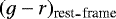 versus Mr rest-frame colour–magnitude diagram (CMD) and computed the stellar mass completeness limit following Zibetti et al. (2009),
 (2)
(2)
where 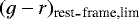 is rest-frame colour limit defined as the colour of the reddest galaxy in the CMD excluding outliers, Mr,lim is the absolute r-band magnitude of the faintest galaxy in the region of the CMD close to the rest-frame colour limit, and the absolute magnitude of the Sun is Mr,⊙ = 4.64. At the redshift of the XLSSsC N01 supercluster and in the entire redshift range adopted in this paper, we assume a conservative stellar mass completeness limit of
  .
.
3 Characterisation of the XLSSsC N01 supercluster: the definition of environment
In this section, we consider Fig. 1 as a reference for the spatial distributions of XLSSsC N01 clusters and galaxies. The upper panels of the figure show the centre of each cluster belonging to XLSSsC N01, along with 3 × r200 circles indicating the cluster spheres of influences. The spectrophotometric sample of galaxies in the top right panel shows, with different colours, galaxies belonging to the four environments we define in this section. We note that atthis stage we are considering the spectrophotometric sample with LePhare outputs presented in the previous sections with a cut at observed magnitudes fainter than the spectroscopic completeness limit, i.e. r = 22.0, which is the most suitable and contains 3120 galaxies; thus, the numbers and fractions written in this section referto this sample, unless otherwise stated. Based on virial properties of clusters together with redshifts of galaxies and their distance from the clusters within XLSSsC N01, we distinguish two membership regions:
Cluster virial members are galaxies whose spectroscopic redshift lies within 3σ of their cluster mean redshift, where σ is the velocity dispersion of their host cluster, and whose projected distance from the cluster centre is <1 r2006. The number of cluster virial members is 130 (4.2% of the spectrophotometric sample). Virial members are marked in the top right panel of Fig. 1 with dark orange diamonds.
Cluster outer members are galaxies whose spectroscopic redshift lies within 3σ from their cluster mean redshift, and whose projected distance from the cluster centre is between 1 and 3 r200. The number of cluster outer members is 133 (4.3% of the spectrophotometric sample), and they are marked in the top right panel of Fig. 1 by black stars.
In order to characterise galaxies in different environments, we extend the definitions of cluster virial and outer members as follows. We consider the redshift range 0.25 ≤ z ≤ 0.35, and we remove galaxies belonging to other nine clusters in the same region, which are not members of the supercluster because of their redshift: 197 galaxies of the 2857 galaxies (6.9%) which are neither in the virial nor in the outer membership regions of XLSSsC N01 clusters are identified as members of these nine clusters and are removed from the sample, so that the remaining 2660 galaxies belong to a general field sample not contaminated by the presence of other X-ray clusters.
Then, we compute projected local densities (LD) in order to further refine the general field environment. We consider all galaxies in the photo-z sample with an observed magnitude r ≤ 22.0, and a photo-z in the range 0.25 ≤ zphot ≤ 0.35: r = 22.0 is the faintest magnitude at which the error in the photo-z estimate is sufficiently low (σ∕(1 + z) ~ 0.03, as reported in Sect. 2.2), while the photo-z range is chosen on the basis of the scatter in the spectroscopic versus photometric redshift plane in order to simultaneously minimise the contamination from galaxies with a photo-z within the selected range but with spectroscopic redshift outside of this range, and maximise the number of galaxies at the redshift of the supercluster. We include in the LD computation also galaxies with no reliable photo-z, but whose spectroscopic redshift is 0.25 ≤ spec-z ≤ 0.35. The photo-z sample of galaxies used in the LD computation is shown in the top left panel of Fig. 1. We define the projected LD relative to a given galaxy as the number of neighbours in a fixed circular region in the sky of radius 1 Mpc at z = 0.2956 (the redshift of XLSSsC N01). We consider all galaxies in the photo-z sample in a slightly larger rectangular region with respect to that defined in Sect. 3 in order to minimise the regions in which boundary corrections had to be performed: 35.0 ≤RA (deg) ≤ 38.25, − 6.5 ≤Dec (deg) ≤−3.5.
The LD is defined as the ratio between the number counts of galaxies Nc in the circle around the considered galaxy and the area A of the circle itself. Count corrections are performed for galaxies in the proximity of the edges in the high declination side of the rectangle (–3.76743 ≤ Dec (deg) ≤ –3.70524) by computing the area of the circular segment that falls outside the field and dividing the LD estimate by the ratio Fc (≤1) between the area actually covered by the data and the circular area.
Figure 2 shows the distribution of the projected LD of our sample. The distribution of cluster virial members is distinct and shifted towards higher values than that for the general field, while the distribution of outer members is broadened in the range of log(LD).
For the general field, we separate galaxies whose log(LD) is higher and lower than the median value of the distribution (log (LD/Mpc−2) ≳ 3.3). The former constitute the “high-density” field, the latter the “low-density” field sample. The number of galaxies belonging to the high-density field is 1436 (46.0%) and to the low-density field is 1224 (39.2%).
The low- and high-density field samples are given together in the top right panel of Fig. 1 along with virial/outer members, and separately in the two bottom panels of the same figure to better visualise their definitions. The high-density field sample traces the presence of several structures around the clusters belonging to XLSSsC N01.
The redshift distributions of galaxies in the different environments is shown in the left panel of Fig. 3. The right panel of the same figure zooms in the redshift distribution of the members, highlighting how the distribution is bimodal, with a second peak in redshift that matches the XLSSC 013 cluster.
From Fig. 1, it can be seen that several groups and clusters are gathered into substructures within the superclusterregion.
The redshift distribution of cluster virial members is arbitrarily divided into seven substructures according to their position in the sky and is shown in Fig. 4. The motivation for this subdivision is twofold: first, groups and clusterswithin each substructure have overlapping virial radii and redshift distributions of member galaxies, which can be assigned to more than one cluster in many cases. In some cases, these clusters (e.g. XLSSC 104 and 168) also share X-ray contours. Second, the subdivision also aims to maximise the visibility of the X-ray contours related to each group and cluster (or substructure), as shown in the figure. For instance, XLSSC 008, 013, 088, and 140 are more distant from the other clusters that are shown together and therefore we show them separately.
The final samples of galaxies that will be used in the scientific analysis is presented in Table 2. We list the number of galaxies in the spectrophotometric catalogue with LePhare and SINOPSIS outputs, respectively, in all the environments defined in this section, both in the magnitude-limited and in the mass-limited samples. We make use of both catalogues because SFRs are available only for the SINOPSIS sample, while the LePhare sample maximises the number of galaxies classified as cluster members.
 |
Fig. 1 Sky distribution of galaxies in the XLSSsC N01 supercluster region. Top left panel: galaxies with a photo-z redshift in the range between 0.25 and 0.35 and used to compute the LD (black points). Top right panel: galaxies with a spectroscopic redshift, colour coded according to their environment (see Sect. 3). Grey crosses are low-density field galaxies, green dots are high-density field galaxies, dark orange diamonds are virial members, and black stars are outer members. In the top panels, black circles show the projected extension in the sky of 3 r200 for each cluster in the superstructure. The two bottom panels show the low- and high-density field samples separately, with the same symbols as the top right panel. |
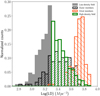 |
Fig. 2 Normalised local density distribution computed using the photo-z sample in redshift range 0.25 ≤ zphot ≤ 0.35. The grey histogram represents the low-density field, the green empty histogram galaxies in the high-density field, the black hatched histogram the cluster outer members, and the orange hatched histogram the cluster virial members. |
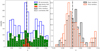 |
Fig. 3 Redshift distribution of the spectrophotometric sample in the region including the XLSSsC N01 supercluster. The centroid redshift of the supercluster is represented with a black dashed line in both panels. Left panel: whole spectroscopic sample (blue histogram), low-density field galaxies (grey distribution), galaxies in the high-density field (green distribution), and galaxies classified as virial and outer members (dark orange and black histogram, respectively). Right panel: zoom in on the virial and outer members, with the same colours used in the left panel (see Sect. 3 for details about the definition of different environments). |
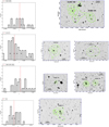 |
Fig. 4 Redshift distribution of XLSSsC N01 cluster virial members divided into seven substructures, and the relative X-ray contours. Left panels: redshift distribution of the virial members in each substructure, as indicated in the labels. The redshift binning is the same in all histograms, and the x-axis extension depends on the redshift range covered by each substructure, for a better visualisation. The mean redshift of the substructure is shown with a vertical red dashed line. Right panels: CFHTLS i-band image of the region surrounding the structures with X-ray contours superposed in green. Blackcrosses indicate the centre of the X-ray emission of point sources. The physical extension of the area in the sky is indicated within each panel. |
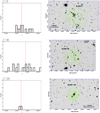 |
Fig. 4 continued. |
Number of galaxies in the different environments above the magnitude and mass completeness limit, respectively, for the sample with successful fits from LePhare and SINOPSIS.
4 Stellar population properties versus environment
In this section, we present the analysis of the stellar population properties of galaxies in different environments using both the magnitude complete sample (r ≤ 20.0) and the mass-limited sample (log(M*∕M⊙) ≥ 10.8).
To distinguish between galaxies at different stages of their evolution, we exploit two different definitions of star-formingand passive galaxies. The first definition is based on the current SFR and stellar mass as measured by SINOPSIS. We define the star formation rate per unit of stellar mass, i.e. the specific star formation rate (sSFR =SFR∕M*), and then consider as star-formingthe galaxies with sSFR > 10−12 yr−1. The remaining galaxies are taken as passive. The second definition is based on galaxy colours as measured by LePhare. To identify the threshold in colour that best separates the blue and red populations, we investigate the correlation between sSFR,  colour and Mr, as shown in Fig. 5, for the subsample analysed by both LePhare and SINOPSIS. Passive galaxies, shown with red points, are mostly clustered at
  , while star-forming galaxies, colour coded according to their sSFR, show a broader distribution. Galaxies having log (sSFR/yr−1) > –9.8 most likely have
  , while galaxies with redder colours have on average log(sSFR/yr−1) ~−10. We therefore consider galaxies with
  to be “red”, and the rest “blue”. With this cut, 80% of passive galaxies are located in the red region of the diagram.
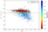 |
Fig. 5 Colour–magnitude diagram for galaxies in the magnitude-limited sample for the subset with both SINOPSIS and LePhare outputs. Red points indicate passive galaxies, while galaxies with log(sSFR) > –12 are colour coded according to their sSFR. The red dotted line shows the separation between red and blue objects. |
4.1 Dependence of the galaxy fractions on environment
We are now in the position of computing the fraction of blue galaxies and star-forming galaxies separately in the different environments identified in the XLSSsC N01 region (see Fig. 6). Focusing on the star-forming fractions in the magnitude-limited sample (top left panel, filled symbols), the fraction of star-forming galaxies in virial members is  , whereas that in low-density field galaxies is
  ; galaxies in the high-density field have an intermediate star-forming fraction (
 ). The fraction of star-forming galaxies in outer members is slightly higher with respect to the other environments (
 ) and in particular with respect to virial members.
Similar trends are visible when the rest-frame colour is considered (top right panel of Fig. 6), where the reduced size of error barswith respect to the star-forming fraction panel at the top left further confirms the results: in the magnitude-limited sample, the fraction of blue galaxies among the virial members is significantly lower than that in the other environments, being only  . By contrast, outer members and high-density field have similar values within the error bars,
  in the former and
  in the latter, and galaxies in the low-density field represent
  of the entire sample. The decrease in the fraction of blue galaxies from the low-density field to the virial members population is a factor of ~2.3 and from outer to virial members a factor of ~1.8.
In the mass-limited sample (shown with empty symbols and dashed error bars) the fractions decrease in all environments and the differences between different environments are smoothed. The only difference that is maintained is between the fraction of blue galaxies in virial members of clusters and the blue fraction in the field. The enhancement and subsequent decrease in the fraction of star-forming/blue galaxies going from the field to outer and then virial members, both in the magnitude and in the mass-complete regimes, point to the direction of an environmental effect that influences the evolution of these galaxies.
In the mass-limited sample, any possible trend is washed out because our stellar mass limit at the redshift of the supercluster selects only high-mass galaxies (log(M*∕M⊙) ≥ 10.8) whose star formation activity, according to the downsizing scenario, was concentrated at earlier epochs and on shorter timescales before the onset of mass quenching. The fraction of star-forming/blue galaxies in the mass-limited sample is indeed lower than the corresponding fraction in the magnitude-limited sample in all environments.
We also note that the fractions of blue and star-forming galaxies are different. In addition to the differences due to the different methods in which the two characteristics are derived, i.e. the star formation rate from spectroscopy and galaxy colours from photometry, the two definitions of star-forming (sSFR) and blue (rest-frame colour) have different physical meanings. Indeed, while the SFR is a snapshot measuring the number of stars produced by the galaxy at the moment it is observed, the colour is also sensitive to the past history of the galaxy itself, especially the recent history, being determined by its predominant stellar population. Furthermore, colour is also influenced by other phenomena, such as metallicity and dust extinction.
Following Nantais et al. (2017), we define the quenching-efficiency parameter (Q.E.) of a given environment with respect to the low-density field as
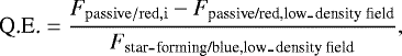 (3)
(3)
where Fpassive∕red,i is the fraction of passive/red galaxies in that environment, 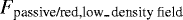 is the fraction of passive/red galaxies in the low-density field, and
  is the fraction of star-forming/blue galaxies in the low-density field. Values of Q.E. in the different environments for the different subsamples are shown in the lower panels of Fig. 6. In both panels, we show as reference the low-density field, which by definition has Q.E. = 0 (Eq. (3)). We note that the error bars associated with the low-density field Q.E. are related to the uncertainties on the star-forming/blue and passive/red fractions, i.e. on the amplitude of the confidence intervals computed through the bootstrapping method.
The efficiency with which cluster virial regions suppress star formation stands out: the Q.E. is significantly higher than in the other environments. The trend is particularly significant using the colour fractions: the Q.E is ~0.5 in cluster virial members, decreases to ~0.2 in outer members, and to ~0.1 in the high-density field.
Values computed using the sSFR fractions are lower: the Q.E. is close to zero in all environments except as traced by virial members, where it reaches a value of ~0.1. In the magnitude and the mass-limited samples, outer members are characterised by a negative Q.E. (decreasing from approximately –0.01 to approximately –0.13 going from one sample to another), suggesting an enhanced star formation activity. In the mass-limited sample (bottom left panel of Fig. 6), however, the negative value of the Q.E. of virial and outer members simply reflects the corresponding star-forming fractions above, and in both cases the large error bars prevent us from drawing solid conclusions.
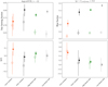 |
Fig. 6 Fraction of star-forming galaxies in different environments, computed with sSFR (left panel) and rest-frame colour (right panel). The fractions obtained using the magnitude-limited sample are represented with filled symbols and solid errors, those obtained using the mass-limited sample are represented by empty symbols and dashed error bars. Errors are derived by means of a bootstrap method. The two lower panels show the quenching efficiency (Q.E.) in different environments, computed with Eq. (3) for both the star-forming and blue samples. The Q.E. of field galaxies, which is by definition set to zero (see Eq. (3)), is shown in both panels as a reference. The error bars on the Q.E of the low-density field depend on the amplitude of the confidence intervals associated with the fractions of star-formingand passive galaxies from bootstrapping. |
4.2 The sSFR– and SFR–mass relations in different environments
In the previous subsection we detected a dependence of the star-forming and blue fractions on environment. We here correlate the galaxy star-forming properties with the stellar mass to further inspect the role of the environment.
First, we focus on the sSFR. In Fig. 7, we show the sSFR–mass relation in the four environments introduced above. Very little difference is observed between the different samples, at least above the mass completeness limit. To better quantify thedifferences, we compute the linear regression fit taking together the different environments above the mass completeness limit. We then plot the distribution of the difference between the sSFR of each galaxy and the value derived from the fit (right panel of Fig. 7). We perform Kolmogorov–Smirnov statistical tests (KS) to compare these distributions, and find that they are all compatible with being drawn from a single parent sample (i.e. the p-values are above the significance level of 0.05). Overall, we conclude that the sSFR–mass relation does not seem to depend on global environment above the galaxy stellar mass limit in our sample, even considering extremely different environments such as X-ray clusters within the XLSSsC N01 supercluster and the field (uncontaminated by X-ray groups or clusters).
Second, we focus on the SFR–mass relation of star-forming galaxies in the four defined environments, shown in Fig. 8. It is evident that galaxies in the different environments are similarly distributed in this plane. In fact, the linear fits performed on the data points of each environment separately are completely superposed when considering virial members and high- and low-density fields, and is slightly steeper when the population of outer members is considered, although the difference can be appreciated only at masses higher than those covered by our sample. We perform a sigma-clipping linear fit to the relation in the mass-complete regime, and compute 1σ confidence intervals, which are shown as blue shaded areas around the solid blue fitting line. Following Paccagnella et al. (2016), we identify galaxies in transition between the star-forming main sequence and the quenched population as those galaxies with log (sSFR/yr−1) > −12 and SFR below –1σ with respectto the SFR–mass fitting line. The fraction is computed as the ratio of this population to the population of galaxies with log (sSFR/yr−1) > −12, in each environment. We find that the incidence of galaxies in transition is not environment dependent, being 0.19 in the low-density field, 0.16
 in the high-densityfield, 0.19
 in cluster outskirts, and 0.18
 in the virial regions of clusters. This trend suggests that in the regions surrounding the XLSSsC N01 supercluster the migration from the star-forming main sequence to the quenched stage occurs similarly from the innermost regions of clusters, to the outskirts, and to the surrounding field.
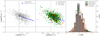 |
Fig. 7 Specific star formation rate (sSFR)–mass relation for galaxies in the low-density field (left panel), and galaxies in the high-density field and cluster virial and outer regions (green dots, orange diamonds, and black stars in the central panel). The vertical and horizontal lines show the stellar mass limit and our adopted separation between star-forming and passive galaxies. The blue dashed line is the fit to the relation of the sample including all the environments. The right panel shows the distribution of the differences between the galaxy sSFRs and their expected values according to the fit giventheir mass. |
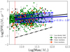 |
Fig. 8 SFR–mass relation for galaxies in the low-density field (grey crosses), in the high-density field (green dots), cluster virial (orange diamonds), and outer members (black stars). The red dashed vertical line shows the stellar mass limit. The blue line is the fit to the relation including all the environments, and the shaded areas correspond to 1σ errors on the fitting line. Linear fits for each environment are shown separately in the figure, colour coded according to the legend. The black dashed line represents the log(sSFR) = –12 limit. |
4.3 Luminosity-weighted age in different environments
Differently from the current SFR and sSFR that give information on the ongoing efficiency of galaxies of producing stars, the luminosity-weighted age (LW-age) provides an estimate of the average age of the stars weighted by the light we observe, and it largely reflects the epoch of the last star formation episode.
Figure 9 contrasts the median LW-age–mass relation in cluster virial members and in high- and low-density fields in the magnitude-limited sample (the galaxy stellar mass limit is shown with a vertical black dashed line). Medians are computed in non-independent stellar mass bins (i.e. there is an overlapping regime between any given stellar mass bin and the two adjacent ones) in order to minimise statistical fluctuations and shaded intervals correspond to the 32nd and 68th percentiles, which is the 1σ confidence interval. The mean LW-age values span the range from ~1.8 × 10⁷ to ~5.6 × 10⁹ yr in the magnitude-limited sample, and from ~109 to ~5.6 × 10⁹ yr in the mass-limited sample. We find overall that the LW-age increases with the galaxy stellar mass in an environmentally independentfashion. No dependences are found even when the outer member population is considered (the results for this population are not shown in the plot for clarity).
To evaluate any possible dependence on galaxy populations, we split galaxies into star-forming/blue and passive/red using the same criteria adopted in previous sections and we plot their median LW-age in the four panels of Fig. 10. While neither the blue nor the red population shows variations in the median value of the LW-age with environment at any stellar mass, environmental dependences are visible when we use the sSFR to separate the star-formingand passive populations. In fact, considering the passive populations, the LW-age of passive galaxies in the virial regions of clusters is systematically lower than that of all other galaxies having the same stellar mass, indicating that these galaxies underwent a recent quenching of the star formation, most likely upon accretion into the cluster.
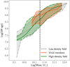 |
Fig. 9 Median luminosity-weighted age–mass relation computed in non-independent stellar mass bins for different environments, as shown in the legend. The stellar mass limit is shown with a vertical black dashed line. Shaded areas are the 32nd and 68th percentiles, corresponding to 1σ error bars. |
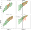 |
Fig. 10 Median luminosity-weighted age–mass relation computed in non-independent stellar mass bins for different environments, as shown in the legend, for star-forming/blue and passive/red galaxies. The stellar mass limit is shown with a vertical black dashed line. Shaded areas are the 32nd and 68th percentiles, corresponding to 1σ error bars. |
5 Summary and discussion
In this work we have presented the characterisation of one of the superclusters identified in XXL Paper XX by means of a FoF algorithm on XXL X-ray clusters. The supercluster, named XLSSsC N01, has a mean redshift of 0.2956, is composed of 14 clusters covering a region of 37 Mpc in RA × 50 Mpc in Dec. Within this region, we characterised the environment of galaxies in 11 clusters, distinguishing among cluster virial members, cluster outer members, high- and low-density field galaxies (which were defined based on their local density). We then characterised the properties of the stellar populations of galaxies in these environments.
First, we computed the fraction of star-forming galaxies, defined in terms of their sSFR, and the fraction of blue galaxies, defined in terms of their  colour. We note that these definitions have different physical meanings. The SFR is a snapshot measuring the number of stars being produced by the galaxy at the moment it is observed, the colour is also sensitive to the past history of the galaxy itself, especially the recent history.
The effect of the environment is mainly visible in galaxies in the densest environments (cluster virial/outer members). Indeed, in the magnitude-limited sample (r ≤ 20.0), the fractions of star-forming and blue galaxies are systematically lower among virial members than in the other environments, indicating star formation quenching in the cluster virialised regions. By contrast, there are hints that the fraction of star-forming galaxies is enhanced among the population of outer members, even with respect to the high- and low-density field. Even though error bars prevent us from stating this on secure statistical grounds, this result suggests an enhancement of star formation when galaxies approach the cluster outskirts. This result is supported by several works at similar and higher redshifts finding that a number of cluster galaxies mostly located in the outskirts and infalling cluster regions still have large amounts of gas, and their star formation can be triggered by the interactions with the ICM, with other galaxies, or by tidal effects (Bai et al. 2007; Marcillac et al. 2007; Fadda et al. 2008; Santos et al. 2013). Marcillac et al. (2007) have found that the mid-infrared selected galaxies in a distant cluster (z ~ 0.83) are associated with infalling galaxies. Bai et al. (2007) have suggested that the cluster environment is able to stimulate the star formation activity in infalling field galaxies before they enter the cluster central regions where gas is stripped and star formation subsequently suppressed. Interestingly, in Koulouridis et al. (2018, XXL Paper XXXV) the same behaviour was found for active galactic nuclei (AGNs) in the XXL clusters, i.e. AGN activity is enhanced in the outskirts while it steeply drops towards the cluster centres. In a redshift range similar to that explored in our work, Fadda et al. (2008) found two filamentary structures in the outskirts of the cluster Abell 1763 (z ~ 0.23), corresponding to infalling galaxies and galaxy groups. The star formation is clearly enhanced in galaxies along the filaments as their associated fraction of starburst galaxies is more than twice that in other cluster regions. They speculate that the relatively high density of galaxies in filaments compared to the general field, and their relatively low velocity dispersion enhances the tidal effect of galaxy encounters and hence the probability of an induced star-forming activity. An enhancement in star formation of galaxies located in the cluster outskirts was also found at high redshift (z ~ 1.4) by Santos et al. (2013), which associated most of the measured FIR star formation in a massive distant cluster with potentially infalling galaxies at the edge of the cluster X-ray emission.
Furthermore, when considering the colour fractions, some additional environmental effects might emerge. In addition to an enhancement of the blue population in the outer members with respect to virial members, the high-density field behaves similarly to the outer members and has a lower incidence of star-forming galaxies than the low-density field. Overall, considering the colours, there is a monotonic trend of increasing star-forming fractions from the clusters, to the high-densityand to the low-density field. We note that the less pronounced enhancement in the blue fraction of outer members compared to their star-forming counterpart may be caused by the fact that the environmental mechanisms triggering star formation are not strong enough to change the colour of these galaxies. Conversely, the star formation enhancement is noticeable when measuring the star formation activity directly from emission lines.
These findings are validated by the quenching efficiency parameter that was computed in all environments using the low-density field as reference. In the local Universe, similar conclusions were drawn by Wetzel et al. (2012), who detected a significant quenching enhancement around massive clusters only for galaxies closer than 2 virial radii from the centre.
In the mass-limited sample (logM*∕M⊙≥ 10.8), the fractions of star-forming and blue galaxies are both lower than their corresponding value in the magnitude-limited sample, quenching efficiency trends are flatter and differences between environments are no longer evident. The stellar mass limit selects only the high-mass end of the galaxy stellar mass function, thus the absence of environmental dependences suggests that the evolution of massive galaxies is mostly completed by this epoch, in agreement with what was previously found (e.g. Brinchmann et al. 2004; Peng et al. 2010; Woo et al. 2013). This scenario is consistent with the downsizing effect (Cowie et al. 1996), according to which galaxies with higher masses are on average characterised by shorter and earlier star formation processes, and become passive on shorter timescales than lower mass galaxies.
We have also investigated the sSFR–mass relation, and find no difference among galaxies in the low- and high- density fields, and in clusters. These results differ from previous findings at similar redshift where a population of cluster galaxies was identified with reduced sSFR with respect to the field at any given stellar mass (e.g. Patel et al. 2009; Vulcani et al. 2010).
The differences might be primarily due to the fact that here we are investigating low-mass clusters and groups, while previous works studied more massive structures. Vulcani et al. (2010), for example, found no differences between the sSFR–mass relation of groups and the field. Furthermore, the fact that the sSFR–mass relation does not show any dependence on environment, while the fraction of star-forming galaxies does, points towards fast quenching mechanisms leading to the formation of a passive population without any evidence of transition in the sSFR-mass diagram. Indeed, the fraction of galaxies in transition from being star-forming to passive, being below 1σ of the SFR–mass relation, is similar throughout the different environments explored in the region surrounding XLSSsC N01.
Finally, we have explored the LW-age–mass relation, finding a systematic increase in the mean LW-age with increasing stellar mass, once again in agreement with the downsizing scenario. Furthermore, while the median LW-age–mass relation of the global population of galaxies is independent of environment, a clear signature of recent quenching of the star formation activity emerges in the passive population of galaxies in the virial regions of X-ray clusters, suggesting the action of environmental processes which are also responsible for the drop in the star-forming fractions highlighted above.
As one of the first studies on stellar populations and star formation activity within superstructures, this analysis lays the groundwork for future investigation into the properties of stellar populations of galaxies on larger samples. In a future work (Guglielmo et al., in prep.), we will investigate whether the characteristics of XLSSsC N01 are shared by other X-ray structures and superstructures by taking advantage of the improved sample statistics of the whole sample of XXL superclusters, with the possibility of exploring a redshift range from z = 0.1 up to z = 0.5. This will also allow a direct comparison with X-ray clusters not belonging to superclusters and will shed light on the role of the large-scale structure in galaxy evolution.
Acknowledgements
XXL is an international project based around an XMM Very Large Programme surveying two 25 deg2 extragalactic fields at a depth of ~5 × 10⁻¹⁵ erg s−1 cm−2 in the [0.5–2] keV band for point-like sources. The XXL website is http://irfu.cea.fr/xxl. Multi-band information and spectroscopic follow-up of the X-ray sources are obtained through a number of survey programmes, summarised at http://xxlmultiwave.pbworks.com/. The Australia Telescope Compact Array is part of the Australia Telescope National Facility, which is funded by the Australian Government for operation as a National Facility managed by CSIRO. GAMA is a joint European-Australasian project based around a spectroscopic campaign using the Anglo-Australian Telescope. The GAMA input catalogue is based on data taken from the Sloan Digital Sky Survey and the UKIRT Infrared Deep Sky Survey. Complementary imaging of the GAMA regions is being obtained by a number of independent survey programmes including GALEX MIS, VST KiDS, VISTA VIKING, WISE, Herschel-ATLAS, GMRT, and ASKAP providing UV to radio coverage. GAMA is funded by the STFC (UK), the ARC (Australia), the AAO, and the participating institutions. The GAMA website is http://www.gama-survey.org/. V.G. acknowledges financial support from the Fondazione Ing. Aldo Gini. B.V. acknowledges the support from an Australian Research Council Discovery Early Career Researcher Award (PD0028506). We acknowledge the financial support from PICS Italy–France scheme (P.I. Angela Iovino). The Saclay group acknowledges long-term support from the Centre National d’Études Spatiales (CNES). E.K. acknowledges support from the Centre National d’Études Spatiales and CNRS. M.E.R.C. and F.P. acknowledge support by the German Aerospace Agency (DLR) with funds from the Ministry of Economy and Technology (BMWi) through grant 50 OR 1514 and grant 50 OR 1608.
References
- Adami, C., Mazure, A., Pierre, M., et al. 2011, A&A, 526, A18 [NASA ADS] [CrossRef] [EDP Sciences] [Google Scholar]
- Adami, C., Giles, P., Koulouridis, E., et al. 2018, A&A, 620, A5 (XXL Survey, XX) [NASA ADS] [CrossRef] [EDP Sciences] [Google Scholar]
- Araya-Melo, P. A., Reisenegger, A., Meza, A., et al. 2009, MNRAS, 399, 97 [Google Scholar]
- Arnouts, S., Cristiani, S., Moscardini, L., et al. 1999, MNRAS, 310, 540 [NASA ADS] [CrossRef] [Google Scholar]
- Bahcall, N. A., & Soneira, R. M. 1984, ApJ, 277, 27 [NASA ADS] [CrossRef] [Google Scholar]
- Bai, L., Marcillac, D., Rieke, G. H., et al. 2007, ApJ, 664, 181 [NASA ADS] [CrossRef] [Google Scholar]
- Bai, L., Rieke, G. H., Rieke, M. J., Christlein, D., & Zabludoff, A. I. 2009, ApJ, 693, 1840 [NASA ADS] [CrossRef] [Google Scholar]
- Baldry, I. K., Balogh, M. L., Bower, R. G., et al. 2006, MNRAS, 373, 469 [NASA ADS] [CrossRef] [Google Scholar]
- Ball, N. M., Loveday, J., & Brunner, R. J. 2008, MNRAS, 383, 907 [NASA ADS] [CrossRef] [Google Scholar]
- Balogh, M. L., Babul, A., Voit, G. M., et al. 2006, MNRAS, 366, 624 [NASA ADS] [CrossRef] [Google Scholar]
- Bell, E. F., & de Jong R. S. 2001, ApJ, 550, 212 [NASA ADS] [CrossRef] [Google Scholar]
- Bertin, E., & Arnouts, S. 1996, A&AS, 117, 393 [NASA ADS] [CrossRef] [EDP Sciences] [Google Scholar]
- Blanton, M. R., Eisenstein, D., Hogg, D. W., Schlegel, D. J., & Brinkmann, J. 2005, ApJ, 629, 143 [NASA ADS] [CrossRef] [Google Scholar]
- Bolzonella, M., Kovač, K., Pozzetti, L., et al. 2010, A&A, 524, A76 [NASA ADS] [CrossRef] [EDP Sciences] [Google Scholar]
- Bond, N. A., Strauss, M. A., & Cen, R. 2010, MNRAS, 409, 156 [NASA ADS] [CrossRef] [Google Scholar]
- Brinchmann, J., Charlot, S., White, S. D. M., et al. 2004, MNRAS, 351, 1151 [NASA ADS] [CrossRef] [Google Scholar]
- Chabrier, G. 2003, PASP, 115, 763 [NASA ADS] [CrossRef] [Google Scholar]
- Chon, G., Böhringer, H., & Nowak, N. 2013, MNRAS, 429, 3272 [NASA ADS] [CrossRef] [Google Scholar]
- Cohen, S. A., Hickox, R. C., Wegner, G. A., Einasto, M., & Vennik, J. 2017, ApJ, 835, 56 [NASA ADS] [CrossRef] [Google Scholar]
- Coil, A. L., Newman, J. A., Croton, D., et al. 2008, ApJ, 672, 153 [NASA ADS] [CrossRef] [Google Scholar]
- Cooper, M. C., Newman, J. A., Croton, D. J., et al. 2006, MNRAS, 370, 198 [NASA ADS] [CrossRef] [Google Scholar]
- Cooper, M. C., Coil, A. L., Gerke, B. F., et al. 2010, MNRAS, 409, 337 [NASA ADS] [CrossRef] [Google Scholar]
- Costa-Duarte, M. V., Sodré, L., & Durret, F. 2013, MNRAS, 428, 906 [NASA ADS] [CrossRef] [Google Scholar]
- Cowie, L. L., Songaila, A., Hu, E. M., & Cohen, J. G. 1996, AJ, 112, 839 [Google Scholar]
- Cucciati, O., Iovino, A., Marinoni, C., et al. 2006, A&A, 458, 39 [NASA ADS] [CrossRef] [EDP Sciences] [Google Scholar]
- Cucciati, O., Marinoni, C., Iovino, A., et al. 2010, A&A, 520, A42 [NASA ADS] [CrossRef] [EDP Sciences] [Google Scholar]
- Cucciati, O., Davidzon, I., Bolzonella, M., et al. 2017, A&A, 602, A15 [NASA ADS] [CrossRef] [EDP Sciences] [Google Scholar]
- Darvish, B., Mobasher, B., Sobral, D., Scoville, N., & Aragon-Calvo, M. 2015, ApJ, 805, 121 [NASA ADS] [CrossRef] [Google Scholar]
- Davidzon, I., Cucciati, O., Bolzonella, M., et al. 2016, A&A, 586, A23 [NASA ADS] [CrossRef] [EDP Sciences] [Google Scholar]
- Davis, M., & Geller, M. J. 1976, ApJ, 208, 13 [NASA ADS] [CrossRef] [Google Scholar]
- De Lucia, G., Poggianti, B. M., Aragón-Salamanca, A., et al. 2007, MNRAS, 374, 809 [NASA ADS] [CrossRef] [Google Scholar]
- Dressler, A. 1980, ApJ, 236, 351 [NASA ADS] [CrossRef] [Google Scholar]
- Dressler, A., Oemler, A., Gladders, M. G., et al. 2009, ApJ, 699, L130 [NASA ADS] [CrossRef] [Google Scholar]
- Einasto, M., Liivamägi, L. J., Saar, E., et al. 2011a, A&A, 535, A36 [NASA ADS] [CrossRef] [EDP Sciences] [Google Scholar]
- Einasto, M., Liivamägi, L. J., Tago, E., et al. 2011b, A&A, 532, A5 [NASA ADS] [CrossRef] [EDP Sciences] [Google Scholar]
- Ettori, S., & Balestra, I. 2009, A&A, 496, 343 [NASA ADS] [CrossRef] [EDP Sciences] [Google Scholar]
- Fadda, D., Biviano, A., Marleau, F. R., Storrie-Lombardi, L. J., & Durret, F. 2008, ApJ, 672, L9 [NASA ADS] [CrossRef] [Google Scholar]
- Fasano, G., Poggianti, B. M., Bettoni, D., et al. 2015, MNRAS, 449, 3927 [NASA ADS] [CrossRef] [Google Scholar]
- Fossati, M., Wilman, D. J., Fontanot, F., et al. 2015, MNRAS, 446, 2582 [NASA ADS] [CrossRef] [Google Scholar]
- Fritz, J., Poggianti, B. M., Bettoni, D., et al. 2007, A&A, 470, 137 [NASA ADS] [CrossRef] [EDP Sciences] [Google Scholar]
- Fritz, J., Poggianti, B. M., Cava, A., et al. 2011, A&A, 526, A45 [NASA ADS] [CrossRef] [EDP Sciences] [Google Scholar]
- Fritz, J., Moretti, A., Gullieuszik, M., et al. 2017, ApJ, 848, 132 [NASA ADS] [CrossRef] [Google Scholar]
- Gal, R. R., & Lubin, L. M. 2004, ApJ, 607, L1 [NASA ADS] [CrossRef] [Google Scholar]
- Gavazzi, G., Boselli, A., Cortese, L., et al. 2006, A&A, 446, 839 [NASA ADS] [CrossRef] [EDP Sciences] [Google Scholar]
- Geach, J. E., Ellis, R. S., Smail, I., Rawle, T. D., & Moran, S. M. 2011, MNRAS, 413, 177 [NASA ADS] [CrossRef] [Google Scholar]
- Gilbank, D. G., Yee, H. K. C., Ellingson, E., et al. 2008, ApJ, 677, L89 [NASA ADS] [CrossRef] [Google Scholar]
- Giles, P. A., Maughan, B. J., Pacaud, F., et al. 2016, A&A, 592, A3 (XXL Survey, III) [NASA ADS] [CrossRef] [EDP Sciences] [Google Scholar]
- Guglielmo, V., Poggianti, B. M., Moretti, A., et al. 2015, MNRAS, 450, 2749 [NASA ADS] [CrossRef] [Google Scholar]
- Guglielmo, V., Poggianti, B.M., Vulcani, B., et al. 2018, A&A, 620, A7 (XXL Survey, XXII) [NASA ADS] [CrossRef] [EDP Sciences] [Google Scholar]
- Guzzo, L., Cassata, P., Finoguenov, A., et al. 2007, ApJS, 172, 254 [NASA ADS] [CrossRef] [Google Scholar]
- Haines, C. P., Gargiulo, A., La Barbera, F., et al. 2007, MNRAS, 381, 7 [NASA ADS] [CrossRef] [Google Scholar]
- Haines, C. P., Pereira, M. J., Smith, G. P., et al. 2015, ApJ, 806, 101 [NASA ADS] [CrossRef] [Google Scholar]
- Hoffman, Y., Lahav, O., Yepes, G., & Dover, Y. 2007, JCAP, 10, 016 [NASA ADS] [CrossRef] [Google Scholar]
- Hogg, D. W., Blanton, M. R., Eisenstein, D. J., et al. 2003, ApJ, 585, L5 [NASA ADS] [CrossRef] [Google Scholar]
- Icke, V., & van de Weygaert, R. 1987, A&A, 184, 16 [NASA ADS] [Google Scholar]
- Ilbert, O., Arnouts, S., McCracken, H. J., et al. 2006, A&A, 457, 841 [NASA ADS] [CrossRef] [EDP Sciences] [Google Scholar]
- Iovino, A., Cucciati, O., Scodeggio, M., et al. 2010, A&A, 509, A40 [NASA ADS] [CrossRef] [EDP Sciences] [Google Scholar]
- Iovino, A., Petropoulou, V., Scodeggio, M., et al. 2016, A&A, 592, A78 [NASA ADS] [CrossRef] [EDP Sciences] [Google Scholar]
- Jian, H.-Y., Lin, L., Oguri, M., et al. 2018, PASJ, 70, S23 [NASA ADS] [CrossRef] [Google Scholar]
- Kartaltepe, J. S., Ebeling, H., Ma, C. J., & Donovan, D. 2008, MNRAS, 389, 1240 [Google Scholar]
- Kauffmann, G., Heckman, T. M., White, S. D. M., et al. 2003, MNRAS, 341, 54 [Google Scholar]
- Kauffmann, G., White, S. D. M., Heckman, T. M., et al. 2004, MNRAS, 353, 713 [NASA ADS] [CrossRef] [Google Scholar]
- Kim, S., Rey, S.-C., Bureau, M., et al. 2016, ApJ, 833, 207 [NASA ADS] [CrossRef] [Google Scholar]
- Koulouridis, E., Poggianti, B., Altieri, B., et al. 2016, A&A, 592, A11 (XXL Survey, XII) [NASA ADS] [CrossRef] [EDP Sciences] [Google Scholar]
- Koulouridis, E., Ricci, M., Giles, P., et al. 2018, A&A, 620, A20 (XXL Survey, XXXV) [NASA ADS] [CrossRef] [EDP Sciences] [Google Scholar]
- Kovač, K., Lilly, S. J., Cucciati, O., et al. 2010, ApJ, 708, 505 [NASA ADS] [CrossRef] [Google Scholar]
- Koyama, Y., Smail, I., Kurk, J., et al. 2013, MNRAS, 434, 423 [NASA ADS] [CrossRef] [Google Scholar]
- La Barbera, F., Pasquali, A., Ferreras, I., et al. 2014, MNRAS, 445, 1977 [NASA ADS] [CrossRef] [Google Scholar]
- Lietzen, H., Tempel, E., Heinämäki, P., et al. 2012, A&A, 545, A104 [NASA ADS] [CrossRef] [EDP Sciences] [Google Scholar]
- Lieu, M., Smith, G. P., Giles, P. A., et al. 2016, A&A, 592, A4 (XXL Survey, IV) [NASA ADS] [CrossRef] [EDP Sciences] [Google Scholar]
- Lin, L., Jian, H.-Y., Foucaud, S., et al. 2014, ApJ, 782, 33 [NASA ADS] [CrossRef] [Google Scholar]
- Longhetti, M.,& Saracco, P. 2009, MNRAS, 394, 774 [NASA ADS] [CrossRef] [Google Scholar]
- Lubin, L. M., Gal, R. R., Lemaux, B. C., Kocevski, D. D., & Squires, G. K. 2009, AJ, 137, 4867 [NASA ADS] [CrossRef] [Google Scholar]
- Luparello, H. E., Lares, M., Yaryura, C. Y., et al. 2013, MNRAS, 432, 1367 [NASA ADS] [CrossRef] [Google Scholar]
- Marcillac, D., Rigby, J. R., Rieke, G. H., & Kelly, D. M. 2007, ApJ, 654, 825 [NASA ADS] [CrossRef] [Google Scholar]
- McGee, S. L., Balogh, M. L., Wilman, D. J., et al. 2011, MNRAS, 413, 996 [NASA ADS] [CrossRef] [Google Scholar]
- Muldrew, S. I., Croton, D. J., Skibba, R. A., et al. 2012, MNRAS, 419, 2670 [NASA ADS] [CrossRef] [Google Scholar]
- Muzzin, A., Wilson, G., Yee, H. K. C., et al. 2012, ApJ, 746, 188 [NASA ADS] [CrossRef] [Google Scholar]
- Nantais, J. B., Muzzin, A., van der Burg, R. F. J., et al. 2017, MNRAS, 465, L104 [NASA ADS] [CrossRef] [Google Scholar]
- Oemler, Jr. A. 1974, ApJ, 194, 1 [NASA ADS] [CrossRef] [Google Scholar]
- Pacaud, F., Pierre, M., Refregier, A., et al. 2006, MNRAS, 372, 578 [NASA ADS] [CrossRef] [Google Scholar]
- Pacaud, F., Clerc, N., Giles, P. A., et al. 2016, A&A, 592, A2 (XXL Survey, II) [NASA ADS] [CrossRef] [EDP Sciences] [Google Scholar]
- Paccagnella, A., Vulcani, B., Poggianti, B. M., et al. 2016, ApJ, 816, L25 [NASA ADS] [CrossRef] [Google Scholar]
- Paccagnella, A., Vulcani, B., Poggianti, B. M., et al. 2017, ApJ, 838, 148 [NASA ADS] [CrossRef] [Google Scholar]
- Pasquali, A., Gallazzi, A., Fontanot, F., et al. 2010, MNRAS, 407, 937 [NASA ADS] [CrossRef] [Google Scholar]
- Patel, S. G., Holden, B. P., Kelson, D. D., Illingworth, G. D., & Franx, M. 2009, ApJ, 705, L67 [NASA ADS] [CrossRef] [Google Scholar]
- Peng, Y.-j., Lilly, S. J., Kovač, K., et al. 2010, ApJ, 721, 193 [NASA ADS] [CrossRef] [Google Scholar]
- Peng, Y.-j., Lilly, S. J., Renzini, A., & Carollo, M. 2012, ApJ, 757, 4 [NASA ADS] [CrossRef] [Google Scholar]
- Pierre, M., Valtchanov, I., Altieri, B., et al. 2004, JCAP, 9, 011 [NASA ADS] [CrossRef] [Google Scholar]
- Pierre, M., Pacaud, F., Adami, C., et al. 2016, A&A, 592, A1 (XXL Survey, I) [NASA ADS] [CrossRef] [EDP Sciences] [Google Scholar]
- Planck Collaboration XVI 2014, A&A, 571, A16 [NASA ADS] [CrossRef] [EDP Sciences] [Google Scholar]
- Poggianti, B. M., Smail, I., Dressler, A., et al. 1999, ApJ, 518, 576 [NASA ADS] [CrossRef] [Google Scholar]
- Poggianti, B. M., von der Linden, A., De Lucia, G., et al. 2006, ApJ, 642, 188 [NASA ADS] [CrossRef] [Google Scholar]
- Poggianti, B. M., Moretti, A., Gullieuszik, M., et al. 2017, ApJ, 844, 48 [NASA ADS] [CrossRef] [Google Scholar]
- Pompei, E., Adami, C., Eckert, D., et al. 2016, A&A, 592, A6 (XXL Survey, VII) [NASA ADS] [CrossRef] [EDP Sciences] [Google Scholar]
- Renzini, A. 2006, ARA&A, 44, 141 [NASA ADS] [CrossRef] [Google Scholar]
- Sánchez-Blázquez, P., Jablonka, P., Noll, S., et al. 2009, A&A, 499, 47 [NASA ADS] [CrossRef] [EDP Sciences] [Google Scholar]
- Santos, J. S., Altieri, B., Popesso, P., et al. 2013, MNRAS, 433, 1287 [NASA ADS] [CrossRef] [Google Scholar]
- Schirmer, M., Hildebrandt, H., Kuijken, K., & Erben, T. 2011, A&A, 532, A57 [NASA ADS] [CrossRef] [EDP Sciences] [Google Scholar]
- Schlegel, D. J., Finkbeiner, D. P., & Davis, M. 1998, ApJ, 500, 525 [NASA ADS] [CrossRef] [Google Scholar]
- Scodeggio, M., Gavazzi, G., Franzetti, P., et al. 2002, A&A, 384, 812 [NASA ADS] [CrossRef] [EDP Sciences] [Google Scholar]
- Scodeggio, M., Vergani, D., Cucciati, O., et al. 2009, A&A, 501, 21 [NASA ADS] [CrossRef] [EDP Sciences] [Google Scholar]
- Scoville, N., Aussel, H., Benson, A., et al. 2007, ApJS, 172, 150 [Google Scholar]
- Scoville, N., Arnouts, S., Aussel, H., et al. 2013, ApJS, 206, 3 [NASA ADS] [CrossRef] [Google Scholar]
- Smith, R. J., Lucey, J. R., Price, J., Hudson, M. J., & Phillipps, S. 2012, MNRAS, 419, 3167 [NASA ADS] [CrossRef] [Google Scholar]
- Sobral, D., Best, P. N., Smail, I., et al. 2011, MNRAS, 411, 675 [NASA ADS] [CrossRef] [Google Scholar]
- Söchting, I. K., Coldwell, G. V., Clowes, R. G., Campusano, L. E., & Graham, M. J. 2012, MNRAS, 423, 2436 [NASA ADS] [CrossRef] [Google Scholar]
- Spitzer, Jr. L.,& Baade, W. 1951, ApJ, 113, 413 [NASA ADS] [CrossRef] [Google Scholar]
- Swinbank, A. M., Edge, A. C., Smail, I., et al. 2007, MNRAS, 379, 1343 [NASA ADS] [CrossRef] [Google Scholar]
- Tanaka, M., Hoshi, T., Kodama, T., & Kashikawa, N. 2007, MNRAS, 379, 1546 [Google Scholar]
- Tasca, L. A. M., Kneib, J.-P., Iovino, A., et al. 2009, A&A, 503, 379 [NASA ADS] [CrossRef] [EDP Sciences] [Google Scholar]
- Verdugo, M., Lerchster, M., Böhringer, H., et al. 2012, MNRAS, 421, 1949 [NASA ADS] [CrossRef] [Google Scholar]
- Vulcani, B., Poggianti, B. M., Finn, R. A., et al. 2010, ApJ, 710, L1 [NASA ADS] [CrossRef] [Google Scholar]
- Vulcani, B., Poggianti, B. M., Fasano, G., et al. 2012, MNRAS, 420, 1481 [NASA ADS] [CrossRef] [Google Scholar]
- Vulcani, B., Poggianti, B. M., Oemler, A., et al. 2013, A&A, 550, A58 [NASA ADS] [CrossRef] [EDP Sciences] [Google Scholar]
- Vulcani, B., Poggianti, B. M., Fritz, J., et al. 2015, ApJ, 798, 52 [NASA ADS] [CrossRef] [Google Scholar]
- Wetzel, A. R., Tinker, J. L., & Conroy, C. 2012, MNRAS, 424, 232 [NASA ADS] [CrossRef] [Google Scholar]
- Wilman, D. J., Balogh, M. L., Bower, R. G., et al. 2005, MNRAS, 358, 88 [NASA ADS] [CrossRef] [Google Scholar]
- Woo, J., Dekel, A., Faber, S. M., et al. 2013, MNRAS, 428, 3306 [NASA ADS] [CrossRef] [Google Scholar]
- Zibetti, S., Charlot, S., & Rix, H.-W. 2009, MNRAS, 400, 1181 [NASA ADS] [CrossRef] [Google Scholar]
r500,scal is defined as the radius of the sphere inside which the mean density is 500 times the critical density ρc of the Universe at the cluster redshift; M500,scal is then defined as  .
.
see http://www.ing.iac.es/weave/science.html for more information on the WEAVE project.
We derive r200 from r500,scal by simply dividing the latter by 0.7 according to the relation adopted in Ettori & Balestra (2009).
All Tables
X-ray and membership properties of clusters within the XLSSsC N01 superstructure.
Number of galaxies in the different environments above the magnitude and mass completeness limit, respectively, for the sample with successful fits from LePhare and SINOPSIS.
All Figures
|
Fig. 1 Sky distribution of galaxies in the XLSSsC N01 supercluster region. Top left panel: galaxies with a photo-z redshift in the range between 0.25 and 0.35 and used to compute the LD (black points). Top right panel: galaxies with a spectroscopic redshift, colour coded according to their environment (see Sect. 3). Grey crosses are low-density field galaxies, green dots are high-density field galaxies, dark orange diamonds are virial members, and black stars are outer members. In the top panels, black circles show the projected extension in the sky of 3 r200 for each cluster in the superstructure. The two bottom panels show the low- and high-density field samples separately, with the same symbols as the top right panel. |
| In the text | |
|
Fig. 2 Normalised local density distribution computed using the photo-z sample in redshift range 0.25 ≤ zphot ≤ 0.35. The grey histogram represents the low-density field, the green empty histogram galaxies in the high-density field, the black hatched histogram the cluster outer members, and the orange hatched histogram the cluster virial members. |
| In the text | |
|
Fig. 3 Redshift distribution of the spectrophotometric sample in the region including the XLSSsC N01 supercluster. The centroid redshift of the supercluster is represented with a black dashed line in both panels. Left panel: whole spectroscopic sample (blue histogram), low-density field galaxies (grey distribution), galaxies in the high-density field (green distribution), and galaxies classified as virial and outer members (dark orange and black histogram, respectively). Right panel: zoom in on the virial and outer members, with the same colours used in the left panel (see Sect. 3 for details about the definition of different environments). |
| In the text | |
|
Fig. 4 Redshift distribution of XLSSsC N01 cluster virial members divided into seven substructures, and the relative X-ray contours. Left panels: redshift distribution of the virial members in each substructure, as indicated in the labels. The redshift binning is the same in all histograms, and the x-axis extension depends on the redshift range covered by each substructure, for a better visualisation. The mean redshift of the substructure is shown with a vertical red dashed line. Right panels: CFHTLS i-band image of the region surrounding the structures with X-ray contours superposed in green. Blackcrosses indicate the centre of the X-ray emission of point sources. The physical extension of the area in the sky is indicated within each panel. |
| In the text | |
|
Fig. 4 continued. |
| In the text | |
|
Fig. 5 Colour–magnitude diagram for galaxies in the magnitude-limited sample for the subset with both SINOPSIS and LePhare outputs. Red points indicate passive galaxies, while galaxies with log(sSFR) > –12 are colour coded according to their sSFR. The red dotted line shows the separation between red and blue objects. |
| In the text | |
|
Fig. 6 Fraction of star-forming galaxies in different environments, computed with sSFR (left panel) and rest-frame colour (right panel). The fractions obtained using the magnitude-limited sample are represented with filled symbols and solid errors, those obtained using the mass-limited sample are represented by empty symbols and dashed error bars. Errors are derived by means of a bootstrap method. The two lower panels show the quenching efficiency (Q.E.) in different environments, computed with Eq. (3) for both the star-forming and blue samples. The Q.E. of field galaxies, which is by definition set to zero (see Eq. (3)), is shown in both panels as a reference. The error bars on the Q.E of the low-density field depend on the amplitude of the confidence intervals associated with the fractions of star-formingand passive galaxies from bootstrapping. |
| In the text | |
|
Fig. 7 Specific star formation rate (sSFR)–mass relation for galaxies in the low-density field (left panel), and galaxies in the high-density field and cluster virial and outer regions (green dots, orange diamonds, and black stars in the central panel). The vertical and horizontal lines show the stellar mass limit and our adopted separation between star-forming and passive galaxies. The blue dashed line is the fit to the relation of the sample including all the environments. The right panel shows the distribution of the differences between the galaxy sSFRs and their expected values according to the fit giventheir mass. |
| In the text | |
|
Fig. 8 SFR–mass relation for galaxies in the low-density field (grey crosses), in the high-density field (green dots), cluster virial (orange diamonds), and outer members (black stars). The red dashed vertical line shows the stellar mass limit. The blue line is the fit to the relation including all the environments, and the shaded areas correspond to 1σ errors on the fitting line. Linear fits for each environment are shown separately in the figure, colour coded according to the legend. The black dashed line represents the log(sSFR) = –12 limit. |
| In the text | |
|
Fig. 9 Median luminosity-weighted age–mass relation computed in non-independent stellar mass bins for different environments, as shown in the legend. The stellar mass limit is shown with a vertical black dashed line. Shaded areas are the 32nd and 68th percentiles, corresponding to 1σ error bars. |
| In the text | |
|
Fig. 10 Median luminosity-weighted age–mass relation computed in non-independent stellar mass bins for different environments, as shown in the legend, for star-forming/blue and passive/red galaxies. The stellar mass limit is shown with a vertical black dashed line. Shaded areas are the 32nd and 68th percentiles, corresponding to 1σ error bars. |
| In the text | |
Current usage metrics show cumulative count of Article Views (full-text article views including HTML views, PDF and ePub downloads, according to the available data) and Abstracts Views on Vision4Press platform.
Data correspond to usage on the plateform after 2015. The current usage metrics is available 48-96 hours after online publication and is updated daily on week days.
Initial download of the metrics may take a while.