| Issue |
A&A
Volume 620, December 2018
|
|
|---|---|---|
| Article Number | A133 | |
| Number of page(s) | 12 | |
| Section | Extragalactic astronomy | |
| DOI | https://doi.org/10.1051/0004-6361/201732241 | |
| Published online | 11 December 2018 | |
The curious case of the companion: evidence for cold accretion onto a dwarf satellite near the isolated elliptical NGC 7796⋆,⋆⋆
1
Departamento de Astronomía, Universidad de Concepción, Concepción, Chile
e-mail This email address is being protected from spambots. You need JavaScript enabled to view it.
2
European Southern Observatory, Karl-Schwarzschild-Str. 2, 85748
Garching, Germany
3
Instituto de Astrofísica, Pontificia Universidad Católica de Chile, Av. Vicuña Mackenna 4860, 7820436
Macul, Santiago, Chile
4
Gemini Observatory, Casilla 603, La Serena, Chile
5
Department of Physics & Astronomy, University of Utah, 115 South 1400 East, Salt Lake City, UT
84112, USA
6
Departamento de Ciencias Físicas, Facultad de Ciencias Exactas, Universidad Andres Bello, Fernández Concha 700, Las Condes
7591538, Chile
Received:
6
December
2017
Accepted:
10
September
2018
Abstract
Context. The isolated elliptical (IE) NGC 7796 is accompanied by an interesting early-type dwarf galaxy, named NGC 7796-DW1. It exhibits a tidal tail, very boxy isophotes, and multiple nuclei or regions (A, B, and C) that are bluer than the bulk population of the galaxy, indicating a younger age. These properties are suggestive of a dwarf–dwarf merger remnant.
Aims. Dwarf–dwarf mergers are poorly understood, but may have a high importance for dwarf galaxy evolution. We want to investigate the properties of the dwarf galaxy and its components to find more evidence for a dwarf–dwarf merger or for alternative formation scenarios.
Methods. We use the Multi-Unit Spectroscopic Explorer (MUSE) at the VLT to investigate NGC 7796-DW1. We extract characteristic spectra to which we apply the STARLIGHT population synthesis software to obtain ages and metallicities of the various population components of the galaxy. This permits us to isolate the emission lines for which fluxes and flux ratios can be measured and to which strong-line diagnostic tools can be applied.
Results. The galaxy’s main body is old and metal-poor. A surprising result is the extended line emission in the galaxy, forming a ring-like structure with a projected diameter of 2.2 kpc. The line ratios fall into the regime of HII-regions, although OB-stellar populations cannot be identified by spectral signatures. The low Hα surface brightnesses indicate unresolved star-forming substructures, which means that broad-band colours are not reliable age or metallicity indicators. Nucleus A is a relatively old (7 Gyr or older) and metalpoor super star cluster, most probably the nucleus of the dwarf, now displaced. The star-forming regions B and C show younger and distinctly more metal-rich components. The emission line ratios of regions B and C indicate an almost solar oxygen abundance, if compared with radiation models of HII regions. Oxygen abundances from empirical calibrations point to only half-solar. The ring-like Hα-structure does not exhibit signs of rotation or orbital movements.
Conclusions. NGC 7796-DW1 occupies a particular role in the group of transition-type galaxies with respect to its origin and current evolutionary state, being the companion of an IE. The dwarf–dwarf merger scenario is excluded because of the missing metal-rich merger component. A viable alternative is gas accretion from a reservoir of cold, metal-rich gas. NGC 7796 has to provide this gas within its X-ray bright halo. As illustrated by NGC 7796-DW1, cold accretion may be a general solution to the problem of extended star formation histories in transition dwarf galaxies.
Key words: galaxies: individual: NGC 7796 / galaxies: kinematics and dynamics / galaxies: star clusters: general / galaxies: ISM
Based on observations collected at the European Organisation for Astronomical Research in the Southern Hemisphere under ESO programme 60.A-9316(A).
The reduced datacube (FITS file) is only available at the CDS via anonymous ftp to cdsarc.u-strasbg.fr (130.79.128.5) or via http://cdsarc.u-strasbg.fr/viz-bin/qcat?J/A+A/620/A133
© ESO 2018
1. Introduction
The first catalogue of isolated elliptical galaxies (IEs; Karachentseva 1973) was based on photographic data and simply contained early-type galaxies with no apparent bright galaxy nearby (see Richtler et al. 2015 for a compact introduction to the literature). IEs in fact may have many dwarf companions (Madore et al. 2004).
NGC 7796 is an IE (Reda et al. 2004). With respect to richness of the globular cluster system, photometric properties, and X-ray properties, it resembles a normal, old elliptical galaxy in a group or cluster (Richtler et al. 2015), in contrast to many other IEs that show signatures of recent interactions and/or younger stellar populations (Salinas et al. 2015). Vader & Chaboyer (1994) list two companions, but only NGC 7796-1 (we respect its nature as a dwarf galaxy and hereafter use NGC 7796-DW1) can be confirmed as a real companion galaxy (see the remarks below) and is classified as dE2. Figure 1 shows NGC 7796 and its companion NGC 7796-DW1 at a projected distance of about 2.1′ or 30 kpc.
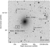 |
Fig. 1. IE NGC 7796 and its dwarf companion, NGC 7796-DW1. |
A detailed image is shown in Fig. 2 (upper left panel). The dwarf galaxy has remarkable properties: it shows a tidal tail (not visible here, but see Richtler et al. 2015), and three central sources which we interpret as “multiple nuclei” and label A, B, and C. However, only object A seems to be a point source, while objects B and C are slightly extended. Therefore only object A seems to be a real nucleus, and we shall use the more appropriate term “region” for the other two objects. The colours of regions B and C indicate intermediate ages of about 1 Gyr, whilst nucleus A and the main body of the galaxy appear older, but with ages that are difficult to estimate from only broad-band colours (more information in Sect. 4). The galaxy also exhibits very boxy outer isophotes.
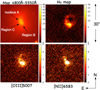 |
Fig. 2. Upper left panel: a MUSE image of NGC 7796-DW1 showing the three different nuclear regions with a square root scaling. Indicated is the mean flux in the interval 4800 Å–5550 Å. As in the other maps, the unit is 10−20 erg s−1 cm−2 Å. Upper right panel: a map of the Hα-flux. The Hα-emission defines an almost complete, but distorted ring with some swellings and knots. Lower left panel: [OIII]5007 map. The [OIII]5007/Hα ratio is constant which indicates local ionising sources. Lower right panel: [NII]6583-map. |
These properties may characterise a merger remnant. Recent work points to the importance of dwarf–dwarf interactions or even dwarf–dwarf mergers: the newly discovered faint dwarf galaxy population in the Fornax cluster core shows signs of correlated clustering (Muñoz et al. 2015; Ordenes-Briceño et al. 2018). Star formation in pairs of dwarf galaxies is enhanced with respect to dwarfs in isolation (Stierwalt et al. 2015; Pearson et al. 2016). Moreover, shells in dwarf galaxies in the Virgo cluster are best understood by dwarf–dwarf mergers (Paudel et al. 2017). These examples show that dwarf–dwarf interaction/mergers are potentially important for the evolution of dwarf galaxies.
NGC 7796-DW1 appears as an example of a transition dwarf galaxy with a mixture of late-type and early-type appearance (e.g. Sandage & Hoffman 1991; Knezek et al. 1999; Lisker et al. 2006; Dellenbusch et al. 2007, 2008; Koleva et al. 2013, 2014).
Here we present a new study with ESO’s new Multi-Unit Spectroscopic Explorer (MUSE), revealing interesting results. The character of NGC 7796-DW1 turns out to be very different from previous understanding. Detailed study of ages, star formation history, and metallicities of its stellar population and the surprising emission lines leads us to conclude that this dwarf galaxy has obtained its younger stellar populations not by a merger, but by accretion of gas suitable for star formation.
As in Richtler et al. (2015), we adopt a distance of 50 Mpc based on the surface brightness fluctuation distance of Tonry et al. (2001), corresponding to 242.4 pc per arcsec.
2. Observations and reductions
NGC 7796-DW1 has been observed with MUSE under the programme 60.A-9316(A), mounted at the Very Large Telescope (VLT) of the European Southern Observatory (ESO) at Cerro Paranal, Chile. The data were first taken as Science Verification data during the night 29/30 June 2014. It turned out that with respect to seeing and photometric quality they did not meet the required standards. The seeing was about 1″̣5 and the night was not photometric. Therefore the observations were repeated during the night 19/20 August 2014, this time reaching a better seeing quality, but still not a high photometric quality. For the present study, we only used the August data.
Table 1 lists object, ESO Phase-3 designation, position, exposure times, and image quality as the FWHM-value of the cube which we finally use.
Summary of observations (ESO program ID 60.A-9316(A)).
MUSE is a mosaic of 24 Integral Field Units (IFUs), covering a field of 1 × 1 arcmin2 in the wide field mode. The pixel scale is 0.2 × 0.2 arcsec2. The spectral resolution varies from R = 2000 at 4700 Å to R = 4000 at 9300 Å which are the extremes of the spectral range covered.
2.1. Reduction
The ESO Phase 3 concept offers through the ESO science archive reduced data products that in our case are four MUSE observing blocks with exposure times of 2 × 900 s each. Originally, we tried to work with a data cube that uses all exposures, so we performed an independent reduction. However, we found that the inclusion of the June data does not improve the final results, so for reasons of clarity and reproducibility, we used the Phase 3 final data cube which only contains the data from August 2014. This data product with the designation given in Table 1 is available in the ESO science archive. For completeness, we briefly describe the reduction process. The reduction has been performed using the pipeline provided by ESO, described by the pipeline manual version 1.6.2, employing the standard EsoRex recipes. The basic reduction consists of applying muse_bias and muse_flat (no correction for dark currents), followed by the wavelength-calibration with muse_wavecal. The line-spread-function has been calculated from the arc spectra using muse_lsf. For the instrument geometry, we used the tables provided by ESO. Twilight exposures were used for the illumination correction, applying muse_twilight. The previous recipes produce frames/tables that now enter the recipe muse_scibasic that performs bias subtraction, flat field correction, wavelength calibration, and more. The recipe muse_scipost performs flux calibration and calculates the final data cube or as a choice, fully reduced pixtables that are combined by muse_exp_combine to produce a data cube with combined individual exposures. The pipeline corrects also for telluric absorption features.
Sky subtraction in the Phase 3 pipeline used the sky exposures and left a weak residuum of the light of NGC 7796 itself and strong sky lines. To remove the sky almost completely, we defined a local sky in the field free of other sources and performed the sky subtraction for each spectrum individually using skytweak under IRAF. Our sky spectrum has been extracted at the position RA = 23:59:15.946, Dec = −55:29:31.0 with QFitsView and a radius of 60 pixels.
The data are not designed for absolute photometry. Since only one standard star is used in the pipeline, we do not expect it to be very precise. We will not draw strong conclusions from absolute fluxes. We expect the relative flux uncertainties to be approximately or better than 5% which is the overall experience (e.g. Weilbacher et al. 2015). We use QFitsView (Ott 2012) for extracting and averaging spectra. The uncertainties for each wavelength element have been calculated using the STAT part of the MUSE cube which gives the variance for each pixel and wavelength element.
2.2. Astrometry and coordinate correction
The absolute astrometric accuracy (for identification purposes only) of the MUSE World Coordinate System (WCS) is relatively good. The USNO star U0300.38162244 (RA: 23:59:13.374, Dec: −55:29:20.87) can be found in the MUSE field. To agree with its coordinates, the MUSE WCS was shifted 1.5″ to the north, 0.11 s to the east. These are the coordinates which we use.
The literature coordinates of the two dwarf companions of NGC 7796 are probably incorrect. Vader & Chaboyer (1994) give coordinates for J1950, which precessed for J2000 would indicate that NGC 7796-DW1 is not identical with APMUKS B235639.76-554544.9 but with a stellar-like object displaced by about 20″ to the south-west (it is indeed a star). The coordinates for NGC 7796-2 indicate a faint galaxy, but shifted by the same displacement as for NGC 7796-DW1, and point to the clear case of a background spiral. We thus conclude that the coordinates of Vader & Chaboyer (1994; which appear in the NED) must be corrected by 11″ to the east and 16″ to the north.
3. Line emission and its morphology
The field around NGC 7796-DW1 covered by MUSE, showing nucleus A and the regions B and C, is displayed in the upper-left panel of Fig. 2. On the VIMOS B-image with its better seeing of 0.8″ (Richtler et al. 2015), region B appears extended, but the true size is difficult to measure. We estimate a FWHM of about 1″, and it is clearly visible that only nucleus A can be a real nucleus or super star cluster. In an outer isophote with a half major axis of 8″ and a half minor axis of 5.5″, nucleus A is offset from the centre by about 1″ (or 240 pc) along the major axis to the north.
A surprising observation is the presence of extended line emission in a major region of the visible galaxy. The other panels of Fig. 2 show maps of Hα, the [OIII]5007 Å-line, and the [NII]6583 Å-line. The Hα-emission is the brightest, which is already an indication that the ionisation resembles more an HII-region than LINER-like line ratios. These maps have been produced by integrating over the full line widths using the line map option of QFitsView with the local continuum subtracted. The Hα emission forms a complete, somewhat elongated ring with the brightest parts in region B. The ring is not complete in the other line maps. The diameter is about 9″ or 2.2 kpc. The ring shows inhomogeneities or swellings, best visible in Hα where continuum-structure-like point sources are not visible. The Hα intensity may therefore reflect the gas density rather than the ionising flux. The emitted flux from nucleus A is not higher than the local background, so nucleus A itself is not a source of line emission as regions B and C are. Its position is also offset from the ring. Further remarks on the ring are given in Sect. 5.5.
Besides nucleus A and the regions B and C, we want to analyse a spectrum from outside these regions, but near the centre where the signal-to-noise ratio (S/N) is still high. Therefore we extracted a spectrum with the coordinate from Table 1 as the centre and a radius of 15 pixels (or 0.727 kpc), and subtracted the spectra of nucleus A, region B, and region C, named R15-minusABC. Furthermore, we investigate a spectrum of the outer parts of the galaxy, which is a spectrum of the annulus 15–30 pixels, named R30-R15. Finally, we analysed a spectrum covering the entire galaxy with a radius of 40 pixels, named R40 (or 1.939 kpc). These six spectra are described in Sect. 4.
4. Population synthesis
For the spectral analysis, which ideally gives ages and metallicities of the population components and, moreover, produces a model spectrum that can be subtracted for the emission line analysis, we employ the STARLIGHT code (Cid Fernandes et al. 2005; Mateus et al. 2006, Version 4). This code fits flux-calibrated spectra using linear combinations of library model spectra. The outputs are mass- and luminosity weighted components, characterised by age and metallicity. Reddening, radial velocity, and fit-related parameters are made available as well. The code has been widely applied in the CALIFA survey (Cid Fernandes et al. 2011; Kehrig et al. 2012; Gomes et al. 2016; Zinchenko et al. 2016).
STARLIGHT does not provide uncertainties. The population decomposition of S/N-limited spectra is plagued by degeneracies between age, metallicity, reddening, spectral resolution, spectral range, and so on. The MUSE spectra are quite red and less appropriate for investigating young populations. An important point is that the broad-band colours of the younger objects in our dwarf do not straightforwardly indicate their ages. A seeing of 0.8″ may mix unresolved young blue structures with the galaxy light and thus let the colours appear redder than the bluest subcomponents. This effect is even more pronounced in the case of the MUSE spectra with their seeing of about 1″. Therefore the task at hand is to answer the question of how much of the young components are visible in the spectra, rather than an analysis of the true star formation history.
Our spectral library consists of 125 model spectra from Bruzual & Charlot (2003) with solar-scaled composition. The metallicities range from z = 0.0004 to z = 0.05, and the ages range from 0.001 Gyr to 18 Gyr. We do not iterate to reduce the number of statistically significant components by deleting all components below a given percentage limit, but show all components that have been involved in the fit. The strong emission lines (Hβ, Hα, [OIII]4959 Å and 5007 Å, [NII]6549 Å and 6583 Å, [SII]6717 Å and 6731 Å) are masked out. The properties of the population synthesis modelling of each co-added spectrum are listed in Table 2 and displayed in Fig. 3. Table 2 lists the identification, the extraction radii, the absorption in the V-band, the radial velocity, χ
2, and two S/N values provided by STARLIGHT. The lower values have been determined from a direct comparison with the model spectra and thus may be the most trustworthy. The higher values result from using the variances of each pixel which are given in the STAT part of the MUSE cube. For each spectrum, we extracted the corresponding spaxels in the STAT section and calculate the resulting variance as  , where N is the number of extracted spaxels and
  the individual variances. The final variance after sky subtraction is the sum of object+sky and sky variance. The square roots of these variances are used by STARLIGHT in the fit.
Properties and fit results of our characteristic spectra.
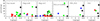 |
Fig. 3. Typical results of a STARLIGHT decomposition for our characteristic spectra. Indicated is the population composition in percentage of light at 5650 Å of all populations involved in the fit. The colours denote metallicities. Black: z = 0.0004; blue: z = 0.008, green: z = 0.02, red: z = 0.05. The individual uncertainties, particularly those at low percentage values, are probably high and determined by many systematics. Therefore this must not be confused with a determination of the star formation history. Rather it confirms what has been suggested by broad-band photometry. Further discussion of this can be found in the text. |
4.1. Nucleus A
The spectrum of nucleus A has been extracted using the circular option of QFitsView with a radius of 2 pixels. The spectrum is dominated by a bright stellar continuum with a strong absorption of Hβ (see Fig. A.1), where the emission line is hardly visible. The emission lines vanish almost completely if a spectrum of the local background is subtracted, which shows that the object itself does not exhibit line emission. Figure 3 indicates a moderately metal-poor and intermediate-age to old object. The weak young contributions may therefore arise from background/foreground populations. If we select only components older than 1 Gyr from Fig. 3 the weighted mean values for age and metallicity are 8.7 Gyr and z = 0.004, respectively. With M R = −12.4, according to Richtler et al. (2015), the associated mass is about several 106 M ⊙, characterising an ω Centauri-like object (Hilker & Richtler 2000). In analogy, one would expect a range of populations to be present. Although NGC 7796-DW1 may possess a globular cluster system on its own, we cannot clearly identify individual point sources as globular clusters, but an object as massive as nucleus A cannot be a normal cluster. It is much more plausible that it was the (now decentred) nucleus of the dwarf elliptical (see more remarks in Sect. 6.1).
It is of interest to try an independent metallicity estimate using the calcium triplet at 8498 Å, 8542 Å, and 8662 Å. In this near-infrared region, contributions from younger populations are negligible. The calibration of Sakari & Wallerstein (2016) indicates that for stellar populations older than 2 Gyr, the sum of the three equivalent widths (EWs) is independent from age and only sensitive to metallicity. Moreover, Da Costa (2016) emphasises the very weak dependence on [Ca/Fe]. The main uncertainty is the definition of the continuum. Unfortunately, the redshift of NGC 7796 superimposes the lines 8542 Åand 8662 Å onto strong sky features. Figure A.1 shows that the continuum of the best-fitting population is placed somewhat too high and the lines themselves are not well fitted. The higher spectral resolution of MUSE in the infrared may also be responsible for the bad representation. We fit the continuum “manually” with splot in IRAF between 8470 Å and 8780 Å and estimate the following EWs: EW(8498) = 1.4 Å, EW(8542) = 2.2 Å, EW(8662) = 2.2 Å. Unresolved spectral features may somewhat increase the EWs and we estimate the uncertainty in all lines to be about 0.2 Å. The calibration of Sakari & Wallerstein (2016) is
 (1)
(1)
This results in a metallicity of [Fe/H] = −1.3 ± 0.6 dex, where also the uncertainties of the coefficients have been considered. This is obviously only a weak constraint, the dominant error source being the slope coefficient in Eq. (1).
4.2. Region B
This region is the brightest spot in Hα, but, as Fig. 2 shows, the intensity peak of the pure emission is somewhat displaced from the optical image. Its spectrum is displayed in Fig. A.3. The population synthesis yields metal-poor old components, but metal-rich and very young components as well. The metal-rich intermediate-age contribution is much stronger than in the case of nucleus A.
There are plausibly several populations that are mixed together by the seeing. The emission line spectrum is that of a typical HII region, so OB populations must be present. The detection of dust would be interesting. The Balmer decrement indicates a weak increase from the standard value of 2.85, but because the reddening law is unknown, the reddening itself remains uncertain. The values in Table 3 have been calculated by applying the standard relation from Momcheva et al. (2013): E(B − V) = 1.97 × log10(H α /H β )/2.85).
Absolute emission line fluxes that have been measured in the spectra normalised by STARLIGHT.
4.3. Region C
The broad-band colour of region C is somewhat redder than that of region B (Table 2). Whether it is older cannot be decided from our data. The very young components are indeed missing. Metalpoor, intermediate-age components are dominating. The strong emission lines have an appearance very similar to those of region B. The Hα peak luminosity is one third of that of region B. We conclude that also region C is actively star forming, but at a lower rate.
4.4. R15minusABC
We want to analyse a spectrum that samples the inner part of the dwarf galaxy but largely avoids the younger regions. Therefore we extract a spectrum with a radius of 15 pixels and subtract the spectra of nucleus A, and regions B and C. Figure 3 shows that now intermediate-age and old metal-poor components are dominant. Calculating the mean for all components older than 1 Gyr, one obtains an age of 9.1 Gyr and a metallicity of z = 0.005.
4.5. R30-R15
This spectrum is the extraction of an annulus between of 15 and 30 pixels in radius. It samples the outer parts of the galaxy and the low-luminosity zone of the north-western parts of the Hα ring. Only old and metal-poor components are found. The mean values for age and metallicity are 11 Gyr and z = 0.002. These values are indicative only. However, they convey the impression of an old, moderately metal-poor dwarf galaxy.
4.6. R40
We extract the total spectrum with a radius of 40 pixels, encompassing an area of about 5000 spaxels. Apart from a measurement of the total Hα-luminosity, it is a useful consistency check for comparison with the other spectra that are more specific regarding the composition of stellar populations. Indeed, no young population contributes, but STARLIGHT finds a range of intermediate-age populations of moderate metal deficiency.
5. Emission lines and diagnostic graphs
5.1. Line fluxes and diagnostic graphs
The lower panels of the spectra depicted in the appendix show the emission line spectra after the model spectra have been subtracted. In Fig. A.1 the emission lines are identified. One finds the usual strong lines. Atomic neutral emission lines are not visible.
We measure the line fluxes in the model-subtracted spectra using splot in IRAF between those wavelengths where the wings of the emission lines reach zero. The fluxes are measured in the spectra normalised to the model spectra. Absolute flux values are then calculated by applying a factor given by STARLIGHT. These factors are given in Table 2.
The line fluxes and line ratios that we use in strong line diagnostics are given in Table 3. The Balmer decrements may indicate the existence of dust in star-forming regions. Balmer decrements Hα/Hβ range from 2.6 (spectrum 5) to 3.2 (spectrum 4). The reddening values have been calculated using a formula from Momcheva et al. (2013; see Sect. 4.2). The outer regions should be dust free, therefore this is qualitatively expected. It is encouraging that the Balmer decrement in the brightest sources, regions B and C, is very close to the standard value of 2.85. This shows a precise separation of stellar and emission line parts in the spectra.
Comparison with photoionisation models that predict strong line fluxes depending on the ionisation rate q1 and oxygen abundance shows good agreement. Dopita et al. (2013) give a summary of the history of strong line diagnostics and a series of diagnostic graphs of which only a few are interesting for us because of the restricted wavelength range. They recommend in particular the graphs [OIII]/Hβ versus [NII/][SII] and [OIII]/[SII] versus [NII/[SII], which permit the cleanest separation between ionisation rate and oxygen abundance. Here, the measurements refer to the sum of both [SII] lines and the [NII] line at 6584 Å, respectively. In addition we show the graph [OIII]/Hβ versus [NII]/Hα to demonstrate that the line ratios remain within the range expected for HII regions.
A new feature in the models of Dopita et al. (2013) is that the electron energies follow a κ-distribution which in the case of κ = ∞ is equal to a Boltzmann distribution. According to Ferland et al. (2016), the thermalisation of electrons with a finite κ-value occurs on shorter timescales than heating or cooling which makes κ = ∞ the preferred choice. Figure 4 shows HII-region models of three different oxygen abundances (0.5, 1, 2; in solar units) for a Boltzmann distribution of electron energies. The ionisation rates range from log(q) = 6.5 to log(q) = 8.5. A good separation of log(q) and oxygen abundance z can be seen in the left and right panels. The middle graph is less suitable for separating these parameters. The solid red line marks the limits between the HII-regions and active galactic nucleus(AGN)-dominated ionisation from Kewley et al. (2001). It is now widely acknowledged that post-AGB stars from older populations also provide an ionising radiation field (e.g. Cid Fernandes et al. 2011) that is not distinguishable from LINERS produced by AGNs. The distinction line is convincingly explained by the fact that high metallicities result in lower temperatures of HII regions and therefore show a degeneracy in the zone of high abundance. Zhang et al. (2017) present photoionisation models of intermediate-age and old stellar populations for some strongline diagnostic diagrams. Their diagrams also indicate that the ionising sources in our case are OB stars.
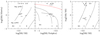 |
Fig. 4. Diagnostic graphs for our six characteristic spectra. These line ratios are compared to HII-region models from Dopita et al. (2013; for a Boltzmann distribution of electrons) with the ionisation parameter log(q) and three oxygen abundances in solar units (0.5, 1, 2) as parameters. The solid lines are lines of constant abundance and varying log(q). The range of log(q) values is indicated in the left panel and is the same for all panels. The solid red line in the middle panel is the line separating HII-regions from AGN-like spectra according to Kewley et al. (2001). The numbers in the upper parts identify the spectra from Table 3 by their sequence. The symbol sizes represent the measurement uncertainty. As noted by Dopita et al. (2013), the right diagnostic graph seems to provide the cleanest separation of log(q) and z. The spectra indicate a solar oxygen abundance for regions B and C and slightly less for the other spectra (Table 4). This abundance variation is not, however, backed up by the empirical calibration of Pilyugin & Grebel (2016). |
For interpolating the tables of Dopita et al. (2013), we use linear expressions in the intervals of interest, which are log(q) < 8.0 and 0.5 < z < 3. For the left panel, we obtain
 (2)
(2)
and for the right panel, we obtain
 (3)
(3)
We do not give values for the middle panel.
The resulting oxygen abundances are listed in Table 4 in the notation 12+log(O/H) with the solar abundance given by 12+log(O/H) = 8.69 (Grevesse et al. 2010). The uncertainties are the standard deviations calculated from error propagation of the uncertainties in Table 3. These small errors do not respect systematics. The uncertainty in the reconstruction of Hβ is probably an important systematic effect. However, one observes only a small scatter in [OIII]/Hβ and moreover, the abundances are much more affected by a shift in the other indices. The abundance difference of about 0.25 dex between spectra 2 & 3 and 4 & 5 is striking. However, this difference is not visible in other calibrations.
Oxygen abundances from comparison of strong line ratios with models and from empirical calibrations.
The mean abundance of 0.6 solar is also consistent with the high metallicities of regions B and C found in the population synthesis.
5.2. Empirical calibration
Pilyugin & Grebel (2016) provide an empirical calibration using three strong line indices that reproduce the oxygen abundances of a sample of calibrating HII regions with temperature-based abundances that have a very small scatter of the order 0.01 dex. They calibrate the following indices: N2 = (6548 + 6583)/Hβ, S2 = (6715+6731)/Hβ, R3 = (4958+5007)/Hβ, where the wavelengths stand for the fluxes of the respective lines (they calibrate further indices involving [O II] 3727 Å that are not relevant here). Because we can measure Hα more precisely than we can Hβ, we adopt Hα = 2.89 × Hβ for N2 and S2, to be consistent with Pilyugin & Grebel (2016). The resulting oxygen abundances from Eq. (6) of Pilyugin & Grebel (2016; upper branch) for our spectra are listed in column 5 of Table 4. The mean abundance is 12+log(O/H) = 8.36 or 0.5 solar with an obviously very small scatter.
This is encouraging, given the very inhomogeneous measurements of the line indices particularly of Hα which depends on the accuracy of the fitting by STARLIGHT. It may be that the relative oxygen abundance systematically differs from the pattern of the calibrating HII regions. Finally, there is the long-standing problem that empirical calibrations give lower oxygen abundances than the photoionisation models (e.g. Bresolin et al. 2009; we also refer to the discussion section of Pilyugin & Grebel 2016). Again, it is safe to say that the oxygen abundance compared with HII regions fits much better to regions B and C than to the other spectra.
5.3. Nitrogen-to-oxygen-ratio
The nitrogen-to-oxygen-ratio is used in the discussion below of whether or not a high N/O ratio can fake a high oxygen abundance (see Sect. 6.1).
We apply the calibration of Zahid et al. (2012; their Eq. (3))
 (4)
(4)
The resulting values are listed as the last column in Table 4.
5.4. Hα-luminosity, total stellar mass
With the adopted distance of 50 Mpc and the Hα-flux from Table 3, the total Hα-luminosity becomes 2.69 × 1038 erg s−1 (before absorption). The uncertainty of this value is considerable, the actual measurement error being only a minor source. We do not know the reddening law, and simply adopting the mean Galactic value (identifying Hα with the R-band), that is, A R = 2.3(B − V) = 0.23 (e.g. Cardelli et al. 1989, see their Table 1 for the scatter of R V -values), may be quite incorrect. The absorption factor in the R-band ranges from 1.2 to 1.5. Adopting a measurement uncertainty of 10% for the absolute flux, the flux interval is (2.9–4.4) × 1038 erg s−1. The distance uncertainty probably dominates the other sources. If one optimistically adopts 10% uncertainty for the distance then the fluxes corresponding to the distances 55 Mpc and 45 Mpc span the range (2.3–5.4) × 1038 erg s−1.
Can this Hα-luminosity be produced by evolved stellar populations as ionising sources? If all Lyman continuum photons from populations older than 108 yr are absorbed and re-emitted in the hydrogen recombination lines, Cid Fernandes et al. (2011) calculate the expected Hα-luminosity (their Eqs. (3) and (4)) as
 (5)
(5)
In this equation, E Hα = 3.026 × 10⁻¹² erg is the energy of an Hα photon, f Hα = 2.206 determines the fraction of energy emitted in Hα, M stellar is the total initial mass, derived from STARLIGHT’s parameter mcortot, and q H = 1041 s−1 M ⊙ is the rate of hydrogen ionising photons. If we approximate the total stellar mass using the Marigo et al. (2008)-models from paper II with the population parameters [Fe/H] = −0.7 and an age of 2.5 Gyr, the M/L-value in the R-band is 1.1 and the mass corresponding to M R = −17.8 becomes 6.9 × 10⁸ M ⊙. The expected Hα-luminosity is subsequently 9.5 × 1037 erg s−1, that is, much lower than the observed one. If we furthermore take into account that the Hα-luminosity is actually produced in only a small fraction of the galaxy’s volume, our adopted stellar mass is much too high for a realistic estimation. One concludes that the ionising sources must be an OB-star population that is unresolved.
It is interesting to compare the emission line properties of our spectra with those of Zhang et al. (2017) who investigate a large sample of star-forming MaNGa galaxies with the intention of distinguishing between effects of HII regions and diffuse ionised gas (DIG). The mix of DIG and emission lines from HII regions may influence diagnostic diagrams of strong lines and so bias, for example, a metallicity determination. The morphological main difference between DIG and HII regions in their sample is the Hα-surface brightness, a low surface brightness being characteristic of DIG. Regarding line ratios, DIG resembles LINER-like line ratios. Comparing the Hα surface-brightness values from Table 3 with those of Zhang et al. (2017), one notes that Table 3 contains only values comparable to the lowest surface brightnesses in the MaNGa sample. On the other hand, the line ratios are well covered by the grids of HII regions, while the DIG regions of Zhang et al. (2017) are not.
That the Hα surface brightnesses are so low may be well explained by spatially unresolved substructure.
If there was contamination by DIG towards high metallicities, we would expect it to be most important in spectra 4 and 5 that sample gas outside the peak luminosities of regions B and C. But the metallicity of spectra 4 and 5 is lower than that of spectra 2 and 3, meaning that at least a shift to higher metallicities through the influence of DIG is not obvious.
An interesting observation is that spectrum 5, which in its emission part samples the fainter outer region of the Hα-ring, also shows a log(q) that is relatively similar to that of regions B and C, although the surface brightness is much lower. A direct conclusion is that the ionising sources, although fainter, must be local. A comparison with Fig. 20 of Zhang et al. (2017) shows that in the diagnostic diagram of log([OIII]/Hβ) versus log([SII]/Hα), both spectra 4 and 5 are still consistent with HII regions and not with a very old population as the ionising source.
5.5. Does the ring rotate?
A ring defines a plane in galaxies that is normally connected with orbital motion, for instance a rotating disk. The natural question therefore arises of whether signs of rotation are visible. Due to the faintness of emission lines in the north-eastern part, only Hα provides the possibility to measure radial velocities along the ring structure. The left panel of Fig. 5 shows the Hα radial velocity map. The gas shows little velocity structure, and the low-surface-brightness zones are not easily visible. In the right panel we plot 81 radial velocities versus three position angles, defined east of north. The spectra have been extracted with very different numbers of spaxels because of the very different surface brightnesses. The horizontal dotted line is the stellar velocity of spectrum 5, assumed to be the systemic velocity. It is apparent that the velocity is not constant, but a rotational velocity structure should not have the same systemic velocity as the lower bound. The gas rather seems to move with a bulky substructure. Data of higher precision would be very useful in constraining the geometry of any such structure.
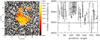 |
Fig. 5. Left panel: Hα radial velocity map. Right panel: radial Hα velocities vs. position angle along the ring. These extractions overlap slightly and give velocities also in the regions of low surface brightness. The horizontal dotted line is the stellar radial velocity of spectrum 5, assumed to be the systemic velocity. A rotation signal is not apparent. |
6. Discussion
6.1. The context of transition dwarf galaxies
NGC 7796-DW1 is clearly an early-type dwarf galaxy with actual or recent star formation, often labelled as a transition dwarf galaxy. The high metallicity of the interstellar medium might be a general indication for accreted material. Here we give a compact literature review. We start with IC 225 for which Gu et al. (2006) determined an oxygen abundance distinctly higher than that expected from the mass-metallicity relation. Dellenbusch et al. (2007, 2008) presented a further six low-mass, oxygen-rich early-type galaxies with recent star formation. A major element of their discussion involved the question of where to locate these galaxies in an evolutionary sequence between dwarf irregulars and dwarf spheroidals. Influential work was presented by Grebel et al. (2003) who used the position in the luminosity-metallicity diagram as well as the HI mass to identify some transition dwarf galaxies on their evolutionary paths towards dwarf spheroidal galaxies.
This scenario was supported by Lisker et al. (2006, 2007) who found a subgroup of disk-like objects among Virgo dwarf ellipticals, sometimes with spiral structure, whose spatial distribution in the cluster resembles irregular and spiral galaxies. Because the cluster environment plausibly triggers the transition from late-type to early-type galaxies, one may conclude that also mass-poor galaxies can undergo transitional processes. Subsequently Peeples et al. (2008) followed with a list of dwarf galaxies extracted from the catalogue of Tremonti et al. (2004) and apparently deviating from a general mass-metallicity relation. The high oxygen abundance has been interpreted by Berg et al. (2011) as an effect caused by a high N/O ratio. However, Zahid et al. (2012) correct for an enhanced N/O ratio and still find a high scatter in the oxygen abundance at low stellar mass, up to about solar metallicity. In our case, the nitrogen abundances from Table 3 can be compared with those in Fig. 10 of Zahid et al. (2012) which shows that they are not enhanced.
The transformation from early-type to late-type galaxies might also be possible. Kannappan et al. (2009) and Wei et al. (2010) identify E/S0 galaxies on the blue sequence and conclude that disk growth in early-type galaxies may occur (see the introduction of Wei et al. 2010 for a compact review of cold gas in early-type galaxies).
Hallenbeck et al. (2012) searched for HI in early-type Virgo dwarfs, finding 12 objects with an HI content typical for dwarf irregulars. Among them, five objects show indications of star formation. They discuss several evolutionary processes for these galaxies and conclude that re-accretion of gas from cosmic filaments is the most plausible process.
For our object, the merging scenario faces the serious difficulty that only one part of the imagined pre-merger galaxies can be identified. Explaining the presence of young, metal-rich components requires a host galaxy of a high mass that corresponds to the higher metallicity. With the bulk of its stars having a metallicity of about [Fe/H] = −0.7, NGC 7796-DW1 fits well to the mass-metallicity relation of dwarf galaxies (Smith Castelli et al. 2008), but the metal-rich stellar component is minor in comparison to the metal-poor component, while it should be more massive.
Moreover, the time sequence of the star formation poses problems for the merger scenario. Considering a merger with two components, a nucleated dwarf elliptical and an irregular dwarf, the merger and coalescence should have happened less than 0.1 Gyr ago, because in merger events the peak of star formation occurs well before coalescence (Stierwalt et al. 2015). Such a relatively young merger should not leave a dwarf with undisturbed isophotes and developed tidal tails. This is a point also made by Dellenbusch et al. (2008) in their morphological study of transition-type dwarfs.
Therefore, excluding a merger, only one viable scenario remains: accretion of cold gas from the inner gaseous halo of NGC 7796, a galaxy this is old and X-ray bright. O’Sullivan et al. (2007) gives, using XMM, an abundance profile that shows nearly solar abundance in the central region and then declines modestly, but with uncertainties which still permit almost solar abundance at larger radii. Cold gas in early-type, X-ray-bright galaxies probably has cooled down from the hot phase (Werner et al. 2014; Smith & Edge 2017). It may reside in disks (Serra et al. 2016; Young et al. 2018), but a disk in NGC 7796 has not yet been identified.
Accretion of cold gas with subsequent star formation is a process whose importance for galaxy evolution has been long underestimated. In cosmology, simulations show the accretion of pristine gas from filaments (Dekel et al. 2009) which trigger star formation in high-z galaxies. For local galaxies, Sancisi et al. (2008) review the process of accretion of cold gas for spiral galaxies with respect to morphological features, but do not mention dwarf galaxies. However, “tadpole” galaxies nicely demonstrate the effect of cold-gas accretion on the morphology of dwarf galaxies (Sánchez Almeida et al. 2013). Another strong indication for infall of cold gas is the existence of metal-poor star-forming regions in otherwise moderately metal-poor dwarf galaxies (Sánchez Almeida et al. 2015).
6.2. Remarks on the star formation history of dwarf galaxies
One classical early-type dwarf galaxy with an extended star formation history is the Andromeda companion NGC 205 with its young nucleus (Melcher et al. 1987; Da Costa & Mould 1988; Monaco et al. 2009). Practically all early-type local-group dwarf galaxies exhibit extended star formation histories (SFHs). A complete literature compilation and extensive discussion is found in Weisz et al. (2014) who investigated the SFHs in about 40 local-group dwarf galaxies. An interesting trend (with exceptions) is that the more massive dwarfs form a lower stellar mass fraction at early times than the less massive dwarfs, a behaviour that is opposite to the “downsizing” of giant galaxies. Weisz et al. explain that due to environmental effects, low mass dwarf spheroidals are preferably found within the virial radii of their host galaxies, while more massive dwarfs populate a larger radius interval. Low-mass galaxies are therefore more susceptible to tidal effects and ram pressure stripping which may quench star formation relatively early.
However, NGC 7796-DW1 is a counterexample to this scenario by showing tidal effects and is also exposed to ram pressure from the hot X-ray gas of NGC 7796. This may therefore suggest that gas accretion is the main driver of star formation in this dwarf galaxy. A dependence on galaxy mass is qualitatively very plausible by assuming that accretion onto deeper potential wells works more efficiently and not only in the central region where one expects the cold gas phase to be densest.
7. Summary and conclusions
We investigate the dwarf companion NGC 7796-DW1 of the IE NGC 7796 by means of IFU data obtained with MUSE at the VLT. The objective is to further probe a possible dwarf–dwarf merger as suspected by Richtler et al. (2015) due to the presence of multiple nuclei and probably a multitude of stellar populations. We distinguish the bulk of the dwarf galaxy: nucleus A and the bluer regions B and C.
The first and surprising finding is that the galaxy, although classified as early-type, is filled with ionised gas, the emission lines being superimposed on top of a stellar continuum or in the case of Balmer lines, embedded in partly deep absorption troughs. Best visible in Hα, the emission forms a ring with a diameter of 9″ or 2.2 kpc of strongly varying brightness.
We define a set of characteristic spectra by sampling the “nuclei” and the stellar population of the galaxy at different radii to achieve a possibly high S/N of the extracted spectra. We performed a population synthesis using STARLIGHT (Cid Fernandes et al. 2005) that fits linear combinations of library spectra to an observed spectrum.
Nucleus A with a mass of about 5 × 10⁶ M ⊙ is the best candidate for the nucleus of this early-type dwarf galaxy. The population synthesis identifies a strongly metal-poor, old component with an intermediate-age contribution. Region B is the region with the highest Hα-luminosity. Its stellar spectrum is still dominated by intermediate-age and old populations, but also shows young (<108 yr) and metal-rich contributions. It is not possible to assign a unique age, but the spectral appearance is the result of spatially unresolved subpopulations. Region C as the secondary peak in the Hα luminosity has a similar metallicity, but the young components are weaker.
STARLIGHT indicates some absorption in regions B and C. Possible ongoing star formation is below visibility. However, a small reddening results in a better agreement between photometric and spectroscopic ages. Younger populations are still present outside the brightness peaks of regions B and C. The outer parts, and thereforethebulkofthegalaxy,resemblethepopulationofnucleus A in that they are metal-poor and are of old to intermediate age.
The emission line strengths can be measured after subtracting the stellar model spectra. The line ratios are typical for metalrich star-forming regions. We compared the line strengths with HII models and empirical calibrations. The oxygen abundance is close to solar which is consistent with the metallicity of the younger stellar populations in the galaxy. OB stars are excluded as ionisation sources, leaving post-AGB stars as the most plausible alternative. This shows that line-ratios might not be reliable for distinguishing between ionising radiation fields of OB stars and post-AGB stars.
The main argument against a dwarf–dwarf merger scenario is the population structure. The mass-metallicity relation suggests that regions B and C cannot have been part of a more metal-rich dwarf; the dwarf must dominate by mass whereas the dominating component is more metal-poor than the comparably low-mass regions B and C.
Star formation in our dwarf galaxy must therefore have been triggered by infall of metal-rich gas. A plausible reservoir of gas with appropriately high metallicity is the gas of the X-ray halo in NGC 7796. We therefore conclude that star formation in our dwarf has been triggered by accretion of cold gas that coexists with the hot X-ray gas. The ring can be understood as the debris of a disk that formed from infalling gas with a certain angular momentum. We suggest that this might be a general recipe for complex SFHs of dwarf galaxies.
The ionisation rate has the unit number of ionising photons per unit area per second and per particle density.
Acknowledgments
We thank the referee for his/her thorough report, in particular for pointing out the misinterpretation of broad-band colours. TR acknowledges support from CONICYT project Basal AFB-170002. He also acknowledges an ESO senior visitorship, during which the data reductions were performed, which was essential for this contribution. T.H.P. gratefully acknowledges support by FONDECYT Regular Project No. 1161817 and by CONICYT project Basal AFB-170002. Dominik Bomans is thanked for discussions on STARLIGHT and literature hints. We use QFitsView (version 3.2, developed by Thomas Ott and Alex Agudo Berbel at the Max Planck Institute for Extraterrestrial Physics, Garching) for extracting and averaging spectra.
References
- Berg, D. A., Skillman, E. D., & Marble, A. R. 2011, ApJ, 738, 2 [NASA ADS] [CrossRef] [Google Scholar]
- Bresolin, F., Gieren, W., Kudritzki, R.-P., et al. 2009, ApJ, 700, 309 [NASA ADS] [CrossRef] [Google Scholar]
- Bruzual, G., & Charlot, S. 2003, MNRAS, 344, 1000 [NASA ADS] [CrossRef] [Google Scholar]
- Cardelli, J. A., Clayton, G. C., & Mathis, J. S. 1989, ApJ, 345, 245 [NASA ADS] [CrossRef] [Google Scholar]
- Cid Fernandes, R., Mateus, A., Sodré, L., Stasińska, G., & Gomes, J. M. 2005, MNRAS, 358, 363 [NASA ADS] [CrossRef] [Google Scholar]
- Cid Fernandes, R., Stasińska, G., Mateus, A., & Vale Asari, N. 2011, MNRAS, 413, 1687 [NASA ADS] [CrossRef] [Google Scholar]
- Da Costa, G. S. 2016, MNRAS, 455, 199 [NASA ADS] [CrossRef] [Google Scholar]
- Da Costa, G. S., & Mould, J. R. 1988, ApJ, 334, 159 [NASA ADS] [CrossRef] [Google Scholar]
- Dekel, A., Birnboim, Y., Engel, G., et al. 2009, Nature, 457, 451 [NASA ADS] [CrossRef] [PubMed] [Google Scholar]
- Dellenbusch, K. E., Gallagher, III., J. S., & Knezek, P. M. 2007, ApJ, 655, L29 [NASA ADS] [CrossRef] [Google Scholar]
- Dellenbusch, K. E., Gallagher, III., J. S., Knezek, P. M., & Noble, A. G. 2008, AJ, 135, 326 [NASA ADS] [CrossRef] [Google Scholar]
- Dopita, M. A., Sutherland, R. S., Nicholls, D. C., Kewley, L. J., & Vogt, F. P. A. 2013, ApJS, 208, 10 [NASA ADS] [CrossRef] [Google Scholar]
- Ferland, G. J., Henney, W. J., O’Dell, C. R., & Peimbert, M. 2016, Rev. Mex. Astron. Astrofis., 52, 261 [Google Scholar]
- Gomes, J. M., Papaderos, P., Kehrig, C., et al. 2016, A&A, 588, A68 [NASA ADS] [CrossRef] [EDP Sciences] [Google Scholar]
- Grebel, E. K., Gallagher, III., J. S., & Harbeck, D. 2003, AJ, 125, 1926 [NASA ADS] [CrossRef] [Google Scholar]
- Grevesse, N., Asplund, M., Sauval, A. J., & Scott, P. 2010, Ap&SS, 328, 179 [NASA ADS] [CrossRef] [Google Scholar]
- Gu, Q., Zhao, Y., Shi, L., Peng, Z., & Luo, X. 2006, AJ, 131, 806 [NASA ADS] [CrossRef] [Google Scholar]
- Hallenbeck, G., Papastergis, E., Huang, S., et al. 2012, AJ, 144, 87 [NASA ADS] [CrossRef] [Google Scholar]
- Hilker, M., & Richtler, T. 2000, A&A, 362, 895 [NASA ADS] [Google Scholar]
- Kannappan, S. J., Guie, J. M., & Baker, A. J. 2009, AJ, 138, 579 [NASA ADS] [CrossRef] [Google Scholar]
- Karachentseva, V. E. 1973, Astrofizicheskie Issledovaniia Izvestiya Spetsial’noj Astrofizicheskoj Observatorii, 8, 3 [NASA ADS] [Google Scholar]
- Kehrig, C., Monreal-Ibero, A., Papaderos, P., et al. 2012, A&A, 540, A11 [NASA ADS] [CrossRef] [EDP Sciences] [Google Scholar]
- Kewley, L. J., Dopita, M. A., Sutherland, R. S., Heisler, C. A., & Trevena, J. 2001, ApJ, 556, 121 [Google Scholar]
- Knezek, P. M., Sembach, K. R., & Gallagher, III., J. S. 1999, ApJ, 514, 119 [NASA ADS] [CrossRef] [Google Scholar]
- Koleva, M., Bouchard, A., Prugniel, P., De Rijcke, S., & Vauglin, I. 2013, MNRAS, 428, 2949 [NASA ADS] [CrossRef] [Google Scholar]
- Koleva, M., De Rijcke, S., Zeilinger, W. W., et al. 2014, MNRAS, 441, 452 [NASA ADS] [CrossRef] [Google Scholar]
- Lisker, T., Glatt, K., Westera, P., & Grebel, E. K. 2006, AJ, 132, 2432 [NASA ADS] [CrossRef] [Google Scholar]
- Lisker, T., Grebel, E. K., Binggeli, B., & Glatt, K. 2007, ApJ, 660, 1186 [NASA ADS] [CrossRef] [Google Scholar]
- Madore, B. F., Freedman, W. L., & Bothun, G. D. 2004, ApJ, 607, 810 [NASA ADS] [CrossRef] [Google Scholar]
- Marigo, P., Girardi, L., Bressan, A., et al. 2008, A&A, 482, 883 [NASA ADS] [CrossRef] [EDP Sciences] [Google Scholar]
- Mateus, A., Sodré, L., Cid Fernandes, R., et al. 2006, MNRAS, 370, 721 [NASA ADS] [CrossRef] [Google Scholar]
- Melcher, N., Richtler, T., & Seggewiss, W. 1987, Mitt. Astron. Ges. Hamburg, 70, 442 [NASA ADS] [Google Scholar]
- Momcheva, I. G., Lee, J. C., Ly, C., et al. 2013, AJ, 145, 47 [NASA ADS] [CrossRef] [Google Scholar]
- Monaco, L., Saviane, I., Perina, S., et al. 2009, A&A, 502, L9 [NASA ADS] [CrossRef] [EDP Sciences] [Google Scholar]
- Muñoz, R. P., Eigenthaler, P., Puzia, T. H., et al. 2015, ApJ, 813, L15 [NASA ADS] [CrossRef] [Google Scholar]
- Ordenes-Briceño, Y., Eigenthaler, P., Taylor, M. A., et al. 2018, ApJ, 859, 52 [NASA ADS] [CrossRef] [Google Scholar]
- O’Sullivan, E., Sanderson, A. J. R., & Ponman, T. J. 2007, MNRAS, 380, 1409 [NASA ADS] [CrossRef] [Google Scholar]
- Ott, T. 2012, Astrophysics Source Code Library [record ascl:1210.019] [Google Scholar]
- Paudel, S., Smith, R., Duc, P.-A., et al. 2017, ApJ, 834, 66 [NASA ADS] [CrossRef] [Google Scholar]
- Pearson, S., Besla, G., Putman, M. E., et al. 2016, MNRAS, 459, 1827 [NASA ADS] [CrossRef] [Google Scholar]
- Peeples, M. S., Pogge, R. W., & Stanek, K. Z. 2008, ApJ, 685, 904 [NASA ADS] [CrossRef] [Google Scholar]
- Pilyugin, L. S., & Grebel, E. K. 2016, MNRAS, 457, 3678 [NASA ADS] [CrossRef] [Google Scholar]
- Reda, F. M., Forbes, D. A., Beasley, M. A., O’Sullivan, E. J., & Goudfrooij, P. 2004, MNRAS, 354, 851 [NASA ADS] [CrossRef] [Google Scholar]
- Richtler, T., Salinas, R., Lane, R. R., Hilker, M., & Schirmer, M. 2015, A&A, 574, A21 [NASA ADS] [CrossRef] [EDP Sciences] [Google Scholar]
- Sakari, C. M., & Wallerstein, G. 2016, MNRAS, 456, 831 [NASA ADS] [CrossRef] [Google Scholar]
- Salinas, R., Alabi, A., Richtler, T., & Lane, R. R. 2015, A&A, 577, A59 [NASA ADS] [CrossRef] [EDP Sciences] [Google Scholar]
- Sánchez Almeida, J., Muñoz-Tuñón, C., Elmegreen, D. M., Elmegreen, B. G., & Méndez-Abreu, J. 2013, ApJ, 767, 74 [NASA ADS] [CrossRef] [Google Scholar]
- Sánchez Almeida, J., Elmegreen, B. G., Muñoz-Tuñón, C., et al. 2015, ApJ, 810, L15 [NASA ADS] [CrossRef] [Google Scholar]
- Sancisi, R., Fraternali, F., Oosterloo, T., & van der Hulst, T. 2008, A&ARv, 15, 189 [NASA ADS] [CrossRef] [EDP Sciences] [Google Scholar]
- Sandage, A., & Hoffman, G. L. 1991, ApJ, 379, L45 [NASA ADS] [CrossRef] [Google Scholar]
- Serra, P., Oosterloo, T., Cappellari, M., den Heijer, M., & Józsa, G. I. G. 2016, MNRAS, 460, 1382 [NASA ADS] [CrossRef] [Google Scholar]
- Smith, R. J., & Edge, A. C. 2017, MNRAS, 471, L66 [NASA ADS] [CrossRef] [Google Scholar]
- Smith Castelli, A. V., Bassino, L. P., Richtler, T., et al. 2008, MNRAS, 386, 2311 [NASA ADS] [CrossRef] [Google Scholar]
- Stierwalt, S., Besla, G., Patton, D., et al. 2015, ApJ, 805, 2 [NASA ADS] [CrossRef] [Google Scholar]
- Tonry, J. L., Dressler, A., Blakeslee, J. P., et al. 2001, ApJ, 546, 681 [NASA ADS] [CrossRef] [Google Scholar]
- Tremonti, C. A., Heckman, T. M., Kauffmann, G., et al. 2004, ApJ, 613, 898 [NASA ADS] [CrossRef] [Google Scholar]
- Vader, J. P., & Chaboyer, B. 1994, AJ, 108, 1209 [NASA ADS] [CrossRef] [Google Scholar]
- Wei, L. H., Kannappan, S. J., Vogel, S. N., & Baker, A. J. 2010, ApJ, 708, 841 [NASA ADS] [CrossRef] [Google Scholar]
- Weilbacher, P. M., Monreal-Ibero, A., Kollatschny, W., et al. 2015, A&A, 582, A114 [NASA ADS] [CrossRef] [EDP Sciences] [Google Scholar]
- Weisz, D. R., Dolphin, A. E., Skillman, E. D., et al. 2014, ApJ, 789, 147 [NASA ADS] [CrossRef] [Google Scholar]
- Werner, N., Oonk, J. B. R., Sun, M., et al. 2014, MNRAS, 439, 2291 [NASA ADS] [CrossRef] [Google Scholar]
- Young, L. M., Serra, P., Krajnović, D., & Duc, P.-A. 2018, MNRAS, 477, 2741 [NASA ADS] [CrossRef] [Google Scholar]
- Zahid, H. J., Bresolin, F., Kewley, L. J., Coil, A. L., & Davé, R. 2012, ApJ, 750, 120 [NASA ADS] [CrossRef] [Google Scholar]
- Zhang, K., Yan, R., Bundy, K., et al. 2017, MNRAS, 466, 3217 [NASA ADS] [CrossRef] [Google Scholar]
- Zinchenko, I. A., Pilyugin, L. S., Grebel, E. K., Sánchez, S. F., & Vílchez, J. M. 2016, MNRAS, 462, 2715 [NASA ADS] [CrossRef] [Google Scholar]
Appendix A: Sample spectra
As sample spectra, we show only the spectra of nucleus A, region B, and R30–R15, whose most significant variation is seen in their population properties.
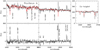 |
Fig. A.1. Spectrum of nucleus A (see Sect. 4). We show only the two most interesting wavelength intervals. Some spectral features are marked for orientation. Upper panel: black solid line marks the observed spectrum, the red solid line the model spectrum. The fluxes are given in units of 10−20 erg−1 cm−2 Å. Lower panel: model spectrum has been subtracted. Here the emission lines are local foreground/background and the cluster itself apparently does not host ionised gas. Right panel: spectral region of the Calcium triplet. This near-infrared region is not well fitted. We therefore measure the EWs directly in the spectrum. |
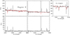 |
Fig. A.2. Spectrum of region B. This is the brightest region. We refer to the caption of Fig. A.1 for more information. |
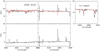 |
Fig. A.3. Spectrum of R30–R15, which is the outer region of the dwarf. The emission lines stem from the faint north-western parts of the gaseous ring. The flux unit here is 10−17 erg−1 s−1 Å. |
All Tables
Absolute emission line fluxes that have been measured in the spectra normalised by STARLIGHT.
Oxygen abundances from comparison of strong line ratios with models and from empirical calibrations.
All Figures
|
Fig. 1. IE NGC 7796 and its dwarf companion, NGC 7796-DW1. |
| In the text | |
|
Fig. 2. Upper left panel: a MUSE image of NGC 7796-DW1 showing the three different nuclear regions with a square root scaling. Indicated is the mean flux in the interval 4800 Å–5550 Å. As in the other maps, the unit is 10−20 erg s−1 cm−2 Å. Upper right panel: a map of the Hα-flux. The Hα-emission defines an almost complete, but distorted ring with some swellings and knots. Lower left panel: [OIII]5007 map. The [OIII]5007/Hα ratio is constant which indicates local ionising sources. Lower right panel: [NII]6583-map. |
| In the text | |
|
Fig. 3. Typical results of a STARLIGHT decomposition for our characteristic spectra. Indicated is the population composition in percentage of light at 5650 Å of all populations involved in the fit. The colours denote metallicities. Black: z = 0.0004; blue: z = 0.008, green: z = 0.02, red: z = 0.05. The individual uncertainties, particularly those at low percentage values, are probably high and determined by many systematics. Therefore this must not be confused with a determination of the star formation history. Rather it confirms what has been suggested by broad-band photometry. Further discussion of this can be found in the text. |
| In the text | |
|
Fig. 4. Diagnostic graphs for our six characteristic spectra. These line ratios are compared to HII-region models from Dopita et al. (2013; for a Boltzmann distribution of electrons) with the ionisation parameter log(q) and three oxygen abundances in solar units (0.5, 1, 2) as parameters. The solid lines are lines of constant abundance and varying log(q). The range of log(q) values is indicated in the left panel and is the same for all panels. The solid red line in the middle panel is the line separating HII-regions from AGN-like spectra according to Kewley et al. (2001). The numbers in the upper parts identify the spectra from Table 3 by their sequence. The symbol sizes represent the measurement uncertainty. As noted by Dopita et al. (2013), the right diagnostic graph seems to provide the cleanest separation of log(q) and z. The spectra indicate a solar oxygen abundance for regions B and C and slightly less for the other spectra (Table 4). This abundance variation is not, however, backed up by the empirical calibration of Pilyugin & Grebel (2016). |
| In the text | |
|
Fig. 5. Left panel: Hα radial velocity map. Right panel: radial Hα velocities vs. position angle along the ring. These extractions overlap slightly and give velocities also in the regions of low surface brightness. The horizontal dotted line is the stellar radial velocity of spectrum 5, assumed to be the systemic velocity. A rotation signal is not apparent. |
| In the text | |
|
Fig. A.1. Spectrum of nucleus A (see Sect. 4). We show only the two most interesting wavelength intervals. Some spectral features are marked for orientation. Upper panel: black solid line marks the observed spectrum, the red solid line the model spectrum. The fluxes are given in units of 10−20 erg−1 cm−2 Å. Lower panel: model spectrum has been subtracted. Here the emission lines are local foreground/background and the cluster itself apparently does not host ionised gas. Right panel: spectral region of the Calcium triplet. This near-infrared region is not well fitted. We therefore measure the EWs directly in the spectrum. |
| In the text | |
|
Fig. A.2. Spectrum of region B. This is the brightest region. We refer to the caption of Fig. A.1 for more information. |
| In the text | |
|
Fig. A.3. Spectrum of R30–R15, which is the outer region of the dwarf. The emission lines stem from the faint north-western parts of the gaseous ring. The flux unit here is 10−17 erg−1 s−1 Å. |
| In the text | |
Current usage metrics show cumulative count of Article Views (full-text article views including HTML views, PDF and ePub downloads, according to the available data) and Abstracts Views on Vision4Press platform.
Data correspond to usage on the plateform after 2015. The current usage metrics is available 48-96 hours after online publication and is updated daily on week days.
Initial download of the metrics may take a while.