| Issue |
A&A
Volume 620, December 2018
|
|
|---|---|---|
| Article Number | A88 | |
| Number of page(s) | 11 | |
| Section | Planets and planetary systems | |
| DOI | https://doi.org/10.1051/0004-6361/201731997 | |
| Published online | 30 November 2018 | |
An alternative stable solution for the Kepler-419 system, obtained with the use of a genetic algorithm
1
Instituto de Astrofísica de La Plata,
CONICET–UNLP, La Plata, Argentina
2
Facultad de Ciencias Astronómicas y Geofísicas, Universidad Nacional de La Plata,
La Plata, Argentina
e-mail: This email address is being protected from spambots. You need JavaScript enabled to view it.
3
Instituto de Astronomía y Física del Espacio,
CONICET–UBA,
Buenos Aires, Argentina
e-mail: This email address is being protected from spambots. You need JavaScript enabled to view it.
Received:
26
September
2017
Accepted:
30
September
2018
Abstract
Context. The mid-transit times of an exoplanet may be nonperiodic. The variations in the timing of the transits with respect to a single period, that is, the transit timing variations (TTVs), can sometimes be attributed to perturbations by other exoplanets present in the system, which may or may not transit the star.
Aims. Our aim is to compute the mass and the six orbital elements of an nontransiting exoplanet, given only the central times of transit of the transiting body. We also aim to recover the mass of the star and the mass and orbital elements of the transiting exoplanet, suitably modified in order to decrease the deviation between the observed and the computed transit times by as much as possible.
Methods. We have applied our method, based on a genetic algorithm, to the Kepler-419 system.
Results. We were able to compute all 14 free parameters of the system, which, when integrated in time, give transits within the observational errors. We also studied the dynamics and the long-term orbital evolution of the Kepler-419 planetary system as defined by the orbital elements computed by us, in order to determine its stability.
Key words: planets and satellites: dynamical evolution and stability / planets and satellites: individual: Kepler-419b / planets and satellites: individual: Kepler-419c
© ESO 2018
1 Introduction
The vast majority of the extra-solar planets known to date were discovered by the method of transits, that is, by detecting the variation of the luminosity of a star due to the eclipse produced when a planet crosses the line of sight. A major contributor of these discoveries was the Kepler space mission, which monitored about 170 000 stars in search of planetary companions (Borucki 2016; Coughlin et al. 2016). The detection of variations in the timing of the transits with respect to a mean period (transit time variations, or TTVs) can be attributed to perturbations by other planetary bodies in the system (Agol et al. 2005; Holman & Murray 2005).
In order to compute the mass and orbital elements of the perturbing bodies from the TTVs, an inverse problem must be solved; at present, only a handful of extrasolar planets have been detected and characterized by solving this inverse problem. Fast inversion methods were developed and tested by Nesvorný & Morbidelli (2008) and Nesvorný & Beaugé (2010) with excellent results for planets in moderately eccentric orbits. Nesvorný (2009) also extended the algorithm to the case of eccentric and inclined orbits. These methods can be briefly summarized as follows. A deviation function is defined as the difference between the modeled transit times and the observed ones; subsequently, the downhill simplex method (e.g., Press et al. 1992) is used to search for its minima. There can be a lack of generality if the modeled mid-transit times are computed by means of a particular truncated planetary perturbation theory to speed up calculations, for example, when a particular multibody mean motion resonance occurs, as can be the case of co-orbitals (see for example, Nesvorný & Morbidelli 2008). Also, as an alternative to the fast inversion methods, a search for the elements of the perturbing body can also be made by direct N-body integration, subsequently refining the result with an optimization algorithm (Steffen & Agol 2005; Agol & Steffen 2007; Becker et al. 2015). In particular, Borsato et al. (2014) solved the inverse problem for the Kepler-9 and Kepler-11 systems by applying a variety of techniques, including a genetic algorithm, although none of the reported results were obtained with the latter. In each experiment, they adjusted a subset of the parameters, keeping the remaining ones fixed. It is worth mentioning that their best solution was obtained by excluding the radial velocities, which suggests that the large errors of these data may contribute to spoiling the fit. A common feature of most methods (see also Carpintero et al. 2014) is that they search in a seven-parameter space for the mass and orbital elements of the unseen planet, whereas they fix the values of the orbital elements and the masses of the transiting planet and of the star, which are estimated before any search is done.
At present, as said, the number of exoplanets discovered by the TTV method is small. The exoplanet.eu database, as of July 1 2018, lists only seven exoplanets discovered solely based on the analysis of the TTVs time series. The first discovery was that of Kepler-46c, with an orbital period of 57.0 days, an eccentricity of 0.0145 and a mass of 0.37 MJ, where MJ is the mass of Jupiter (Nesvorný et al. 2012). In the case of Kepler-51 (Masuda 2014), two transiting planets were already known and their TTV series revealed the existence of a third planetary body, KOI-602.02, with a mass of 0.024 MJ, an eccentricity of 0.008, and an orbital period of 130.19 days; later it was discovered that KOI-602.02 is also a transiting body. All planetary components in this system have low orbital eccentricities. In the case of the WASP-47 system, there are three transiting planets (Adams et al. 2015), two of them exhibiting measurable TTVs due to the existence of an additional body. To estimate the mass and orbital properties of WASP-47e, the fourth planet in the system, Becker et al. (2015) first modeled the TTV series of WASP-47b and WASP-47d using TTVFAST (Deck et al. 2014) and then used a Markov chain Monte Carlo algorithm (Foreman-Mackey et al. 2013) to search for the solution of the inverse problem. This methodology allowed them to put an upper limit on the mass of WASP-47e. It is worth noting that Becker et al. (2015) used the TTVs not only to determine orbital elements, but also to determine masses, therefore allowing the confirmation of the planetary nature of the transiting objects. Finally, the case of the Kepler-419 system is the most peculiar one, due to the large eccentricity of the transiting planet, with a reported value of 0.833, a mass of 2.5 MJ, and a period of 69.76 days (Dawson et al. 2012). Its TTV time series revealed the existence of a more distant and massive planet, with an approximate orbital period of 675.5 days (Dawson et al. 2014, hereafter D14).
The peculiarities of the presently known exoplanetary systems in general, and in multiple systems in particular, place interesting constraints on the formation scenarios that may produce the observed distributions of various parameters as semimajor axes, eccentricities, masses, planetary radii, and so on. In particular, the formation and evolution scenario of high-eccentricity planets is, at present, quite heavily debated in the literature (Jurić & Tremaine 2008; Ford & Rasio 2008; Matsumura et al. 2008; Moeckel et al. 2008; Malmberg & Davies 2009; Terquem & Ajmia 2010; Ida et al. 2013; Teyssandier & Terquem 2014; Duffell & Chiang 2015). Naturally, the refinement in the knowledge of the masses and orbital elements of the known exoplanets would allow more realistic investigations to be performed, for example, regarding their stability (see for example, Tóth & Nagy 2014; Mia & Kushvah 2016; Martí et al. 2016).
It was recognized early on that the case of the Kepler-419 system offers a superb model to solve the inverse problem (Dawson et al. 2012). Firstly, the interaction between the two planets is secular in nature. This can be corroborated through their orbital evolution since the semi-major axes remain constant and the eccentricity librates with a single constant period, which guarantees that the problem is not degenerate. If the interaction contained mean-motion resonant terms, which depend on the mean longitudes of the system, different combinations of these fast angles might result in the same characteristic period, and therefore the solution would not be unique. Secondly, the time span of the data covers about two periods of the more distant, nontransiting planet, so enough information is available to solve the inverse problem accurately.
In orderto solve this inverse problem, we use a genetic algorithm (Charbonneau 1995) and seek maxima of a so-called fitness function, defined as the reciprocal of the sum of the squares of the deviations between the modeled transit times and the observed ones. The efficiency of the method is such that the problem can be solved very accurately even if the number of unknowns is increased to include all the dynamical parameters of the system, that is, the orbital elements and masses of the two planets and the mass of the star, with the exception of the longitude of the ascending node of the transiting planet, which can be fixed arbitrarily. To obtain the modeled mid-transit times used to compute the fitness function, we integrate the three-body gravitational problem in an inertial frame. We disregard interactions due to body tides, relativistic approximations, and non-gravitational terms arising from radiation transfer between the star and the planets.
By using as initial guesses sets of parameters close to those previously estimated for the Kepler-419 planetary system, we have been able to find a solution that, when integrated in time, gives the observed central transit times entirely within the observational errors. The solution consists in a set of orbital parameters of both planets and their masses and the mass of the central star. We then studied the long-term orbital evolution of the Kepler-419 planetary system as defined by the orbital elements computed by us, thus characterizing its general dynamics and determining its stability.
2 Method
2.1 The genetic algorithm
Since the space of parameters is multidimensional, an optimization algorithm based on random searches is inescapable. We refrained from using the popular MCMC algorithm because it requires some prior information about the distribution of the parameters, which in our case is completely unknown and probably very far from a simple multidimensional Gaussian. Instead, we chose to work with a genetic algorithm approach that does not require any previous knowledge of the background distribution. A genetic algorithm is an optimization technique that incorporates, in a mathematical language, the notion of biological evolution. One of its remarkable features is its ability to avoid getting stuck in local maxima, a characteristic which is very important in solving our problem (see Sect. 3). We used a genetic algorithm in this work based on PIKAIA (Charbonneau 1995), which we briefly describe here.
As a first step, the optimization problem has to be coded as a fitness function, that is a function  , where the domain D is the multidimensional space of the n unknown parameters of the problem, and such that f has a maximum at the point corresponding to the optimal values. Let x be a point in this domain, which is called an individual. The algorithm starts by disseminating K individuals x i, i = 1, …, K at random. The set of K individuals is called the population, and, at this stage, they represent the first generation. Two members of the population are then chosen to be parents by selecting them at random but with probabilities that depend on their fitnesses. The coordinates of the parents are subjected to mathematical operations resembling the crossover of genes and mutation. The resulting two points correspond to two new individuals (i.e., two new points x i ∈ D). Subsequently, a new pair of parents are chosen, not necessarily different from earlier parents, and the cycle is repeated until a number K of off spring, that is, a new generation, have been generated. The new individuals will be, on average, fitter than those of the first generation (Charbonneau 1995). The loop starts again from the selection of a pair of parents, and the procedure continues until a preset number of generations has passed, or until a preset tolerance in the value of the maximum of the fitness function is achieved. The fittest individual of the last generation constitutes the result, which in general will not be an exact answer, but an approximation to it. For a detailed account of the numerical procedures, we refer the reader to Charbonneau (1995).
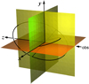 |
Fig. 1 Geometry of the problem. The plane of the sky is the plane of reference of the orbits, which we choose to be the (x, y) plane. The observer looks toward the positive z-axis, the center of mass of the system being at the origin of coordinates. A transiting planet (small ellipse) has an inclination close to 90°, that is, it has an orbit almost perpendicular to the plane of the sky. Another planet (big ellipse) perturbs it. The ascending node of the transiting planet defines the x-axis on the plane of the sky; the line of the nodes of the other planet is marked with a black segment on this plane. |
2.2 Setup and computation of the mid-transit times
The problem is stated as follows: given the (nonperiodic) observed transit times of a planet tobs,i, i = 1, …, N, and assuming the presence of a second, unseen planet which is held responsible for the lack of periodicity, we want to find the mass and the six orbital parameters of each planet, and the mass of the central star.
The geometry of the problem is set as follows. Using Cartesian coordinates, we take the plane of the sky as the (x, y) plane (the reference plane); the z-axis points from the observer to the sky. On the reference plane, we set the x-axis as pointing to the direction of the ascending node of the transiting planet (TP), that is, toward the point at which it crosses the plane of the sky moving away from the observer. We note that this defines the longitude of the ascending node of this planet as zero. The y-axis is chosen so that a right-handed basis is defined (Fig. 1). The perturbing planet has no constraints.
Let p = {a, e, i, Ω, ω, M, m} be the semimajor axis, eccentricity, inclination, longitude of the ascending node, argument of the periastron, mean anomaly and mass of a planet, respectively, which we simply refer to as “elements” for brevity. Given the elements of the TP p t, those of the perturbing planet p p, and the mass of the star m⋆, one can integrate the respective orbits, and compute the transits tcom,i, i = 1, …, N of the TP. The fitness function F[tcom(pt, pp, m⋆), tobs] is defined inour problem as
![Mathematical equation: \begin{equation*} F=\left[\sum_{i=1}^N (t_{\textrm{obs},i}-t_{\textrm{com},i})^2 \right]^{-1}.\end{equation*}](/articles/aa/full_html/2018/12/aa31997-17/aa31997-17-eq2.png) (1)
(1)
The larger the value of F, the better the solution. A value F →∞ would indicate that a set {pt, pp, m⋆} had been chosen so that the resulting transits would coincide perfectly with the (central values of) the observed ones; this would be the “exact” solution. In terms of the genetic algorithm, an individual x is a set {pt, pp, m⋆}.
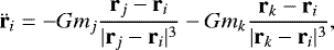
Once the first generation is generated at random, each individual is taken in turn and its fitness is computed by integrating the respective orbits. To this end, we first transform the elements of the planets to Cartesian coordinates, with the center of mass at the origin (e.g., Murray & Dermott 1999). In this inertial frame and from these initial conditions, we integrate the system as a full three-body problem using the standard equations of motion where for each body i (TP, perturbing planet and star),
 (2)
(2)
with G the gravitational constant, and mj,k, rj,k the masses and position vectors of the other two bodies. These allow an easy computation of the transits, that is, the times when the TP is in the z < 0 semispace and the x coordinate of the TP, xt, and that of the star, x⋆, coincide. We note that the star moves during the integration, so the transits are not, in general, the instants when xt = 0. To determine the instants of transit, we used Hénon’s method of landing exactly on a given plane (in our case, the plane x = x⋆) in only one backstep after the plane was crossed, a method that he developed to compute surfaces of section (Hénon 1982, see Appendix A). The numerical integrations were carried out using a Bulirsch–Stoer integrator (Press et al. 1992) with a variable time step initially set at Δt = 0.005 yr ≃ 1.83 days; the relative energy conservation was always below 10−11.
Each integration starts wherever the orbital elements put the planets (tinit; see Fig. 2), that is, the elements corresponding to each individual are defined at tinit. So far, this time has no Julian date assigned. When the first transit t1,com is found during the integration, this instant is made to coincide with the first observed transit t1,obs, therefore receiving the BJDTDB 2 454 959.3308 label, that is, the date of the first observed transit reported in D14. In this way, the tinit instant also gets a BJDTDB, thus defining the date to which the elements belong. Later, the integration comes to a second transit t2,com, which would not be in general coincident to the observed t2,obs – unless the initial elements are the exact ones. The integration continues until N transits have been computed (where N coincides with the number of observed transits); then, the fitness of the individual is computed by means of Eq. (1).
We briefly mention here the values of the parameters of the genetic algorithm used in our experiments(for details of their meaning, we refer the reader to Charbonneau 1995). We chose K = 5000 individuals per generation, six (decimal) digits to define the genotype of each parameter, a probability of genetic crossover equal to 0.95, a generational replacement in which, after a new full generation has been computed, the K best individuals among the new and the old generations are taken, and we have selected the parents with a probability directly proportional to their fitnesses. We also chose a selection pressure of 80% of the maximum possible value1. The mutation rate was variable, from 0.5 to 5%. The algorithm was considered finished when 2000 generations had passed.
The entire algorithm, written in FORTRAN, was parallelized with the MPI paradigm. Using four Intel Core i7 processors at 2.30 GHz, a typical run of 2000 generations lasts approximately 14 h.
 |
Fig. 2 Time axis for each individual. The initial time of the integration and the first computedtransits are marked with vertical lines (lower labels); the observed transits are marked with dots (upper labels). At the first computed transit, a Julian date is assigned to t1,com corresponding to t1,obs. In this way, the instant tinit defining the elements gets a BJDTDB equal to the first transit minus the time elapsed since the start of the integration. |
Intervals (min, max) into which the elements of the planets and the mass of the star were chosen for the first run.
3 Experiments and results
We applied our algorithm to the system Kepler-419 (D14). This system has at least two planets: a transiting warm Jupiter (Kepler-419b) and a nontransiting super-Jupiter (Kepler-419c). The transiting planet has a period of approximately 70 days, and there are N = 21 observed transits, spanning the first 16 quarters of the Kepler data.
We generated the initial conditions for each of our individuals by randomly choosing values from a given interval for each element. The intervals were initially chosen centered on the values reported by D14, their Table 4, and according to the errors reported by them, except the angle Ωb which is zero by definition. A set of test runs of the algorithm systematically gave values of periastrons, mean anomalies, Ωb, mb, and ib at the border of the corresponding intervals. Therefore, we expanded these initial intervals, in the case of the first five angles to at least one quadrant (Table 1). Finally, after investigating the evolution of several solutions, we found that a difference close to 180° between the arguments of the periastrons of the planets was instrumental to ensure the long-term stability of the system. Therefore, as an additional constraint, we imposed that the initial values of those arguments differ in 180°.
Our first run with the extended intervals gave a value of F = 358 397 for the best individual, with times measured in days. Computing the mean of the deviations between the resulting mid-transit times and the observed mid-transit times yielded about 24 s. We repeated the run but with angular initial intervals no greater than one quadrant, choosing the latter according to the final value of the first run. A fitness F = 478 590 was obtained. Then a third run was performed, for which new initial intervals were chosen centered in the values of the output of the last run, and with widths reduced to 80% of the last values. This new run gave F = 546 261, equivalent to a mean deviation of about 20 s between observed and computed mid-transit times. New attempts gave no substantial improvement, so we considered the outcome of this third run as our result.
To estimate statistical errors for the parameters, we first perturbed each input time with noise taken from a Gaussian distribution with zero mean and a dispersion equal to the (maximum) error reported for it in Table 5 of D14. With this new set of mid-transit times, we repeated the experiment and registered the output values of the parameters. We repeated this 50 times, and computed the dispersion of the results. As a check, we inverted the procedure and perturbed the elements inside the resulting intervals of error, surprisingly obtaining solutions that went well beyond the errors of the observed transits. This behavior is expected if, for example, there are correlations among the elements, because independent perturbations lead them out of their correlated values, and then the solution deteriorates. We looked for correlations by taking pairs of elements in turn, constructing a dense grid of values for each pair inside their respective statistical intervals as computed above, and computing for each point of the grid the root mean square of the differences between the resulting transits and the central values of the observed ones (i.e.,  ). We found several pairs of elements with strong correlation. As an example, in Fig. 3 we show the case eb versus ec, where it is seen that the perturbations should lie on a very narrowband if one wishes to keep around 1 min of mean error. With the help of these plots, we computed the true errors of the parameters. The final values of the parameters together with their errors are listed in the fourth column of Table 1, corresponding to BJDTDB 2 454 913.8629. As a reference, we also integrated the system from this epoch to BJDTDB 2 455 809.4010, that is, the epoch at which the elements of D14 are defined. The resulting values are equal to the ones listed (within errors), with the obvious exception of the mean anomalies which gave values of Mb = 69° and Mc = 345°.
Figure 4a shows the resulting differences tcom,i − tobs,i between the computed transits and the observed ones, compared with the errors in the observed transits reported in D14. The first transit has a null error by construction. In order to compare the quality of our solution against the previous one of D14, we also computed the transits resulting from integrating the orbits that correspond to the central values of their Table 4. Since they reported that their elements are Jacobian, and we are not aware of a definition of Jacobian elements, we interpreted this as referring to Jacobian Cartesian coordinates. Thus, we first converted the elements of D14 to Jacobian Cartesian coordinates taking the interior planet and the star as the first subsystem of the ladder; these were in turn converted to astrocentric Cartesian and integrated. Nevertheless, the differences between Jacobian and astrocentric Cartesian coordinates are, in this system, negligible. We also tried an integration by directly converting the elements of D14 as if they were astrocentric, and no appreciable differences were found. Another point to take into account is that these elements are given at BJDTDB 2 455 809.4010, so the integration includes both a backward and a forward period. The forward integration gave a first transit about 13 days after the initial epoch, which came as a surprise because that is the interval between the initial epoch and the previous transit. During this process, we realized that the coordinate system of D14 is defined with the x-axis at the descending node, and the angles ω, M, and i are measured toward the − z semispace (see Fig. 10 of D14). This implies that a transit is defined as the passage through y = 0 from x > 0 to x < 0. On the contrary, in a coordinate system like ours (x-axis at the ascending node and angles measured toward the + z semispace), the transit occurs from x < 0 to x> 0. In terms of orbital elements, the only difference is in the argument of the periastron: the argument of D14 is obtained by adding π to ours (see Appendix B); this should be taken into account if our elements are to be compared with those of D14. Considering this difference, we integrated the D14 system again, finding a large drift which causes a difference of the order of one day at the extreme points (Fig. 4b). In light of our results regarding the errors of the elements, we suspected that this drift was probably due to a lack of enough decimal digits in the solution. We integrated the solution of D14 again with more digits (Dawson, priv. comm.) and found a sensible improvement: less than a quarter of a day in the backward integration. This supports the need to give all the necessary digits in Table 1 in order to reproduce the desired solution. All the integrations were also reproduced with the Bulirsch-Stoer method implemented in the MERCURY package (Chambers 1999), with a fixed time step of 1 day and an added routine to reap the transits.
Table 2 provides a list of the transits computed with our solution. We also include future transits to allow comparison against prospective new observations.
We also computed the radial velocity (RV) of the star with respect to the center of mass of the system. Since the latter is at the origin of an inertial frame fixed in space with respect to the observer, the RV is simply the velocity ż ⋆. This is plotted in Fig. 5 (solid line), together with the observed values (points with error bars).
Considering that the inclination of the orbit of the TP in our solution is 87.° 4 (cf. 88.° 95 in D14), one may wonder whether the TP transits at all. We computed the impact parameter b directly from the dynamical simulation as the difference between the y-coordinate of the TP minus the y-coordinate of the star at each transit (both are points without dimension in the simulation), and compared them to two different stellar radii: 1.75 R⊙, that is, the final value reported in D14, and 1.39 R⊙, the minimum value found by those authors among the different fits. Figure 6 shows that the exoplanet indeed transits in spite of the low inclination of its orbit. We also computed the duration of the transits, using the formulas of Winn (2010), taking into account that a different coordinate system is used in that work, namely, our ω is Winn’s ω − π (see Appendix B). With R⋆ = 1.75 R⊙, we obtained a total duration of 3.76 h; with R⋆ = 1.39 R⊙, the eclipse lasts 2.84 h, very close to the reported value in Dawson et al. (2012) of 2.92 h.
Why did we use mid-transit times instead of TTVs? The TTV signal is the result of computing the differences between the observed transit times (O) and a linear ephemeris value which corresponds to a periodic orbit (C) for each transit epoch. In this way it is expected that the deviation of the transits of a planet from a Keplerian orbit can be visualized in an O−C plot. However, the actual linear ephemeris is unknown, and therefore it is estimated from the mid-transit times themselves, usually by a least-squares fit. Unless the deviations are evenly distributed above and below the real ephemeris (in a least-squares sense), this procedure does not guarantee that the computed linear fit will coincide with the Keplerian period.
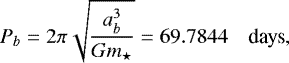
For Kepler-419b, for example, the mean period between transists – obtained from the linear fit of the O− C data – is 69.7546 days (D14). However, computing the Keplerian motion from our solution yields
 (3)
(3)
that is, about 42 min of difference. That is why we chose to work with the bare mid-transit times instead of going through the TTVs.
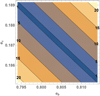 |
Fig. 3 Contours of the root mean square of the differences between the resulting transits and the central values of the observed ones (i.e., |

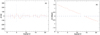 |
Fig. 4 Panel a: differences tcom,i−tobs,i between thecomputed transits and the observed ones (plus signs joined with a solid line), and errors in the observed transits as reported in D14 (crosses with error bars). Panel b: as in panel a but with the parameters taken from D14. We note thedifferent scales on the plots. |
Transits computed by integrating our model.
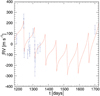 |
Fig. 5 RV of the final system (solid curve), and observed values (dots with error bars). |
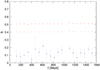 |
Fig. 6 Impact parameter b, computedas the fraction of the star radius at which the point representing the planet sits when it transits. The upper (red) crosses are computed considering a stellar radius R⋆ = 1.39 R⊙. The set of pluses correspond to a stellar radius R⋆ = 1.75 R⊙. The lower (blue) crosses with error bars are the values obtained by D14 with the TAP software (Gazak et al. 2012). |
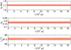 |
Fig. 7 Long-term evolution of the semimajor axis, the eccentricity, and the inclination of Kepler-419c using the elements listed in Table 1 as initial conditions. |
4 Dynamics and long-term evolution
We studied the general orbital dynamics and the long-term evolution of the system using as initial conditions the orbital and physical elements that we have determined, in order to evaluate its stability. We integrated the orbits with the Bulirsch–Stoer method implemented in the MERCURY package (Chambers 1999), with a fixed time step of 0.1 days for a simulated timespan of 200 Myr.
We find that Kepler-419c, the more massive and distant planet, follows a stable secular behavior (Fig. 7), that is, the mean values of the semimajor axis, the eccentricity, and the inclination remain remarkably constant. Figure 8, corresponding to the first 16 000 yr of integration, shows the short-term evolution of the elements. It is seen that the semimajor axis has a mean value of ≃1.71 au, whereas the variation about this value has a small amplitude, of less than 0.05 au. The eccentricity librates about 0.2, the main component having a period of about 8000 yr and an amplitude of less than 0.05. The inclination also librates about a value of ≃ 87.° 5 with a period of the order of 3800 yr. The longitude of the periastron rotates with a period of about 7000 yr. The node librates about a value of ≃13° with a period similar to that of the inclination. As expected, the plot of the Delaunay’s variable  shows that it is not conserved, that is, the planet is not in the Kozai (1962) resonance. This is further confirmed by the lack of both coupled oscillations between the eccentricity and the inclination, and libration of the longitude of the periastron.
In contrast, the long-term evolution of the inner planet Kepler-419b (Fig. 9) shows a slow variation of its semimajor axis, probably due to the proximity to a high-order mean-motion resonance, since the ratio of periods between Kepler-419band Kepler-419c is close to one tenth. On the other hand, the eccentricity and the inclination are as constant in the long term asin Kepler-419c. Figure 10 shows the short-term dynamics. The periods involved are clearly almost the same as in the other planet. The semimajor axis maintains a mean value of 0.375 au, with very small variations around it. The eccentricity librates harmonically about 0.81, the main component having a period of about 8000 yr and an amplitude of about 0.03; there is also a clear second-order libration, with a period of approximately 200 yr. The inclination also librates about a value of ≃ 87.5°, with a period somewhat larger than 2000 yr and a rather large amplitude of ≃ 25°. The longitude of the periastron rotates with a period of about 7000 yr. The node librates about a value of ≃ 15° with a period similar to that of the inclination. Delaunay’s variable  is not conserved and, in general, the eccentricity and inclination do not oscillate in counter-phase and the longitude of the periastron does not librate, except for an event at about 60 Myr where there is a temporary capture in the Kozai’s resonance.
It is remarkable that both planets are in a  secular resonance, that is, both longitudes of the periastron rotate at the same rate. We define the regular elements:
We plot these elements in Fig. 11, where it can be clearly seen that ϖb − ϖc librates about a value of 180° with a small amplitude.
It is worth noticing that other solutions found by changing, for example, the seed of the random number generator or the amplitude of the initial intervals, were sometimes better than the reported one with respect to the fit of the mid-transit times, but they were unstable. The details of some of these unstable solutions are given in Table 3. After inspecting several outcomes, it was apparent that an (close) antialignment of the arguments of the periapses all along the evolution of the system was a necessary condition for the stability of the system: this ensuredthat the distance of closest approach between the planets occured at the maximum possible value, when one of them was at the periastron and the other one at the apoastron. Although a more detailed dynamical description of this condition is necessary, it is beyond the scope of this investigation. In Table 3 we also report the outcome of the long-term integration of the elements of the Kepler-419 system as proposed in Almenara et al. (2018), which turns out to be unstable as well. We note that in the latter case the longitude of the node of Kepler-419b is 180°, due to a different choice of the coordinate system.
As an example, Fig. 12 shows the apoastron Qb of Kepler-419b and the periastron qc of Kepler-419c as a function of the time for the unstable system S1; as can be seen, the planets suffer a close encounter, the inner one falling on the star as a consequence of this. Therefore, a solution like this must be discarded inspite of it yielding a better fit.
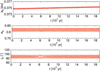 |
Fig. 9 Long-term evolution of the semimajor axis, the eccentricity and the inclination of Kepler-419b, using the elements listed in Table 1 as initial conditions. |
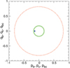 |
Fig. 11 pb vs. qb (red dots), pc vs. qc (green dots),and pbc vs. qbc (blue dots). |
Elements of unstable planetary systems Si with a large value of the fitness F.
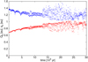 |
Fig. 12 Qb (red dots) and qc (blue dots) as a function of time, for an unstable system. |
5 Conclusions
We have solved the inverse problem of the TTVs for the Kepler-419 system, obtaining remarkable agreement with the observed times of transit, since the mean of the deviations is of the order of 20 s.
We must note that the methodology that we applied to solve the inverse problem was able to produce an accurate and stable solution after a reasonable computing time because we started with a good first guess, as provided by D14. If this information were not available, the extremely complex landscape of the 13-dimensional fitness function would turn any attempt to find a solution into a daunting if not impossible task. We also note that the observed transits of Kepler-419b cannot be reproduced using the orbital elements and masses of the initial solution (i.e., the values of the parameters from D14) evolved with the equations of the full three-body gravitational problem integrated with both the Bulirsch–Stoer subroutine from Press et al. (1992) and the MERCURY package using the option “BS2” (Chambers 1999).
By finding a solution for the problem, we were able to compute a set of values for the orbital elements of both planets and the mass of the star that give central transit times within the observational errors.
The dynamics of the Kepler-419 system computed with the initial conditions listed in Table 1 is qualitatively similar to the one assuming the initial elements found by D14. However, the differences are nonnegligible since the mid-transit times differ considerably, meaning that the validity of one or the other set should require confirmation through future observations of the transits of Kepler-419b. It would also be interesting to decipher the quality of the fit of the light curve of the individual transits to models constructed using the orbital and physical parameters determined in this investigation, which was based solely on the series of transits.
Acknowledgements
We want to thank the anonymous referee who pointed out to us several important aspects of the original draft which greatly improved our work. We also want to thank Prof. Dr. Juan Carlos Muzzio who gave us useful advice. D.D.C. acknowledges support from the Consejo Nacional de Investigaciones Científicas y Técnicas de la República Argentina through grant PIP 0426 and from the Universidad Nacional de La Plata through grant Proyecto 11/G153. M.M. acknowledges the funding by PICT 1144/13 (ANPCyT, MinCyt, Argentina) and PIP 269/15 (Conicet, Argentina).
Appendix A Hénon’s step
We briefly explain here Hénon’s (1982) method of landing exactly on a given plane in only one step of integration.
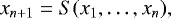
Consider a dynamical system defined by the n differential equations:
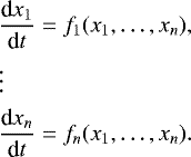 (A.1)
(A.1)
We want to find the intersections of a solution of Eqs. (A.1) with an (n− 1)-dimensional (hyper) surface, defined by the equation
 (A.2)
(A.2)
To this end, we first define a new variable,
 (A.3)
(A.3)
and add the corresponding differential equation to the system (A.1):
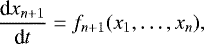 (A.4)
(A.4)
where
 (A.5)
(A.5)
This allows defining the surface S as the (hyper)plane
 (A.6)
(A.6)
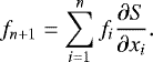
Now, we want to turn xn+1 into the independent variable: if this is done, all we have to do to land exactly on S = 0 is to integrate the new equations from whatever value xn+1 has to 0. The transformation can be easily achieved by dividing Eq. (A.1) by the new Eq. (A.4), and inverting the latter:
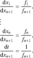 (A.7)
(A.7)
The variablet has now become one of the dependent variables, and xn+1 the independent one.
In practice, one integrates until a change of sign is detected for S. Then, one shifts to the system (A.7), and integrates it one step from the last computed point, taking
 (A.8)
(A.8)
as the integration step. After that, one reverts to the system (A.1) to continue the integration.
The only error involved is the integration error for the system (A.7), which is usually of the same order as the integration error for one step of the system (A.1).
Appendix B Coordinate systems
We briefly describe here the differences between the three coordinate systems mentioned in the text, due to the fact that these differences are somewhat subtle and not easy to recognize.
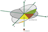 |
Fig. B.1 The standard system of reference. |
B.1 The standard celestial mechanical system of reference
Murray & Dermott (1999) show in their Fig. 2.13 the standard coordinate system used in Celestial Mechanics (hereafter the standard system); Fig. B.1 reproduces it.
The relevant definitions, taken from Murray & Dermott (1999), are (a) the x−y plane defines the reference plane, and the + x semiaxis defines the reference line of the system; (b) the point where the orbit crosses the reference plane moving from below to above (− z to z) is the ascending node; (c) the angle between the reference line and the radius vector to the ascending node is the longitude of the ascending node, Ω; (d) the angle between the radius vector to the ascending node and that to the pericentre of the orbit is the argument of pericentre, ω; (e) the angle between the radius vector to the pericentre and that to the planet is the true anomaly, f. The planet orbits in the sense of increasing ω (or f).
In the present work, we use this standard coordinate system. We put the reference plane in the sky (a standard choice) and the observer in Earth at the − z semiaxis. With this, a transit is defined as the point on the orbit where ω + f = 3π∕2. Alternatively, the transit may also be defined as the point where x = 0 and ẋ > 0, or as the point where x = 0 and z < 0.
B.2 The Winn’s system of reference
Murray & Correia (2010) describe Keplerian orbits using the standard system. In the same book, Winn (2010) says that “As in the chapter by Murray and Correia, we choose a coordinate system centered on the star, with the sky in the x− y plane and the + z axis pointing at the observer”. But then Winn defines the + x semiaxis pointing to the descending node, giving Ω = 180° when the line of the nodes coincide with the + x axis. It is worth noting that the descending node in this system is the same point as the ascending node in the standard system, because the z-axis is inverted. Besides, Winn defines the conjunctions as the condition x = 0, which gives him f + ω = π∕2 for the transit; this means that the argument of pericentre is measured as in the standard system from the nodal line, that is, from the ascending node. The transit can also be defined in this system as the point where x = 0 and ẋ > 0 (as in the standard system), or where x = 0 and z > 0 (contrary tothe standard system). Another difference is that a prograde orbit in the standard system (with respect to the + z axis) is a retrograde orbit in this system. Maintaining the same physical situation than in Fig. B.1, the elements of the Winn system are shown in Fig. B.2.
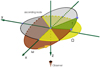 |
Fig. B.2 Winn’s system of reference. |
In terms of values of angles (subindex W stands for Winn, subindex S for standard), we have ΩW = ΩS + π, and ωW = ωS + π.
B.3 The Dawson et al.’s system of reference
D14 used a third system of reference. Their axes have the same orientation as in the standard system (x−y plane on the sky, + z axis pointing away from the observer), and also the reference line is on the + x axis. However the argument of the pericentre is measured from the nodal line toward the − z semispace (see their Fig. 10). Therefore, the nodal line is in reality the anti-nodal line, and the + x axis correspond to the descending node, as in Winn, though the + z axis is similar to that in the standard system. Figure B.3 shows this third system.
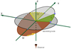 |
Fig. B.3 System of reference used in D14. |
In the standard and Winn systems, the line of nodes (ascending node) is the origin from which ω is measured. In the Dawson et al. system, this origin is the anti-nodal line. Therefore, the two classes of systems are defined in an essentially different way. The same can be said about the definition of Ω: in the standard and Winn systems, this angle is defined between the + x axis and the nodal (ascending) line; in the Dawson et al. system, it is defined between the + x axis and the anti-nodal (descending) line: Dawson et al. define Ω = 0 at this descending node, contrariwise to the standard definition. The transits are at ω + f = π∕2, as in Winn. Also they can be defined as the points where x = 0 and ẋ < 0 (contrary to the standard system), or where x = 0 and z < 0 (as in the standard system).
In terms of values of angles (subindex D standing for Dawson et al.), we have ΩD = ΩS = ΩW − π and ωD = ωW = ωS + π.
References
- Adams, F. C., Becker, J. C., Vanderburg, A., Rappaport, S., & Schwengeler, H. M. 2015, in AAS/Division for Extreme Solar Systems Abstracts, 3, 102.04 [Google Scholar]
- Agol, E., Steffen, J., Sari, R., & Clarkson, W. 2005, MNRAS, 359, 567 [NASA ADS] [CrossRef] [Google Scholar]
- Agol, E., & Steffen, J. H. 2007, MNRAS, 374, 941 [NASA ADS] [CrossRef] [Google Scholar]
- Almenara, J. M., Díaz, R. F., Hébrard, G., et al. 2018, A&A, 615, A90 [NASA ADS] [CrossRef] [EDP Sciences] [Google Scholar]
- Becker, J. C., Vanderburg, A., Adams, F. C., Rappaport, S. A., & Schwengeler, H. M. 2015, ApJ, 812, L18 [NASA ADS] [CrossRef] [Google Scholar]
- Borsato, L., Marzari, F., Nascimbeni, V., et al. 2014, A&A, 571, A38 [NASA ADS] [CrossRef] [EDP Sciences] [Google Scholar]
- Borucki, W. J. 2016, Rep. Prog. Phys., 79, 036901 [NASA ADS] [CrossRef] [Google Scholar]
- Carpintero, D. D., Melita, M. D., & Miloni, O. I. 2014, in Rev. Mex. Astron. Astrofis. 43, 68 [Google Scholar]
- Chambers, J. E. 1999, MNRAS, 304, 793 [NASA ADS] [CrossRef] [MathSciNet] [Google Scholar]
- Charbonneau, P. 1995, ApJS, 101, 309 [NASA ADS] [CrossRef] [Google Scholar]
- Coughlin, J. L., Mullally, F., Thompson, S. E., et al. 2016, ApJS, 224, 12 [NASA ADS] [CrossRef] [Google Scholar]
- Dawson, R. I., Johnson, J. A., Fabrycky, D. C., et al. 2014, ApJ, 791, 89 [NASA ADS] [CrossRef] [Google Scholar]
- Dawson, R. I., Johnson, J. A., Morton, T. D., et al. 2012, ApJ, 761, 163 [NASA ADS] [CrossRef] [Google Scholar]
- Deck, K. M., Agol, E., Holman, M. J., & Nesvorný, D. 2014, ApJ, 787, 132 [CrossRef] [Google Scholar]
- Duffell, P. C., & Chiang, E. 2015, ApJ, 812, 94 [Google Scholar]
- Ford, E. B., & Rasio, F. A. 2008, ApJ, 686, 621 [NASA ADS] [CrossRef] [Google Scholar]
- Foreman-Mackey, D., Hogg, D. W., Lang, D., & Goodman, J. 2013, PASP, 125, 306 [CrossRef] [Google Scholar]
- Gazak, J. Z., Johnson, J. A., Tonry, J., et al. 2012, Adv. Astron., 2012, 697967 [NASA ADS] [CrossRef] [Google Scholar]
- Hénon, M. 1982, Phys., 5, 412 [Google Scholar]
- Holman, M. J., & Murray, N. W. 2005, Science, 307, 1288 [NASA ADS] [CrossRef] [PubMed] [Google Scholar]
- Ida, S., Lin, D. N. C., & Nagasawa, M. 2013, ApJ, 775, 42 [NASA ADS] [CrossRef] [Google Scholar]
- Jurić, M., & Tremaine, S. 2008, ApJ, 686, 603 [NASA ADS] [CrossRef] [Google Scholar]
- Kozai, Y. 1962, AJ, 67, 591 [Google Scholar]
- Malmberg, D.,& Davies, M. B. 2009, MNRAS, 394, L26 [NASA ADS] [CrossRef] [Google Scholar]
- Martí, J. G., Cincotta, P. M., & Beaugé, C. 2016, MNRAS, 460, 1094 [NASA ADS] [CrossRef] [Google Scholar]
- Masuda, K. 2014, ApJ, 783, 53 [NASA ADS] [CrossRef] [Google Scholar]
- Matsumura, S., Takeda, G., & Rasio, F. A. 2008, ApJ, 686, L29 [NASA ADS] [CrossRef] [Google Scholar]
- Mia, R., & Kushvah, B. S. 2016, MNRAS, 457, 1089 [NASA ADS] [CrossRef] [Google Scholar]
- Moeckel, N., Raymond, S. N., & Armitage, P. J. 2008, ApJ, 688, 1361 [NASA ADS] [CrossRef] [Google Scholar]
- Murray, C. D., & Correia, A. C. M. 2010, Keplerian Orbits and Dynamics of Exoplanets, ed. S. Seager, 15 [Google Scholar]
- Murray, C. D., & Dermott, S. F. 1999, Solar System Dynamics [Google Scholar]
- Nesvorný, D. 2009, ApJ, 701, 1116 [NASA ADS] [CrossRef] [Google Scholar]
- Nesvorný, D., & Beaugé, C. 2010, ApJ, 709, L44 [NASA ADS] [CrossRef] [Google Scholar]
- Nesvorný, D., Kipping, D. M., Buchhave, L. A., et al. 2012, Science, 336, 1133 [NASA ADS] [CrossRef] [PubMed] [Google Scholar]
- Nesvorný, D., & Morbidelli, A. 2008, ApJ, 688, 636 [NASA ADS] [CrossRef] [Google Scholar]
- Press, W. H., Teukolsky, S. A., Vetterling, W. T., & Flannery, B. P. 1992, Numerical Recipes in Fortran 77: The Art of Scientific Computing, 2nd edn. (Cambridge, UK: Cambridge University Press) [Google Scholar]
- Steffen, J. H., & Agol, E. 2005, MNRAS, 364, L96 [Google Scholar]
- Terquem, C., & Ajmia, A. 2010, MNRAS, 404, 409 [NASA ADS] [Google Scholar]
- Teyssandier, J., & Terquem, C. 2014, MNRAS, 443, 568 [NASA ADS] [CrossRef] [Google Scholar]
- Tóth, Z., & Nagy, I. 2014, MNRAS, 442, 454 [NASA ADS] [CrossRef] [Google Scholar]
- Winn, J. N. 2010, Exoplanet Transits and Occultations, ed. S. Seager (Tucson, AZ: University of Arizona Press), 55 [Google Scholar]
The selection pressure controls how much the fitness influences the probability of being selected as a new parent.
All Tables
Intervals (min, max) into which the elements of the planets and the mass of the star were chosen for the first run.
All Figures
|
Fig. 1 Geometry of the problem. The plane of the sky is the plane of reference of the orbits, which we choose to be the (x, y) plane. The observer looks toward the positive z-axis, the center of mass of the system being at the origin of coordinates. A transiting planet (small ellipse) has an inclination close to 90°, that is, it has an orbit almost perpendicular to the plane of the sky. Another planet (big ellipse) perturbs it. The ascending node of the transiting planet defines the x-axis on the plane of the sky; the line of the nodes of the other planet is marked with a black segment on this plane. |
| In the text | |
|
Fig. 2 Time axis for each individual. The initial time of the integration and the first computedtransits are marked with vertical lines (lower labels); the observed transits are marked with dots (upper labels). At the first computed transit, a Julian date is assigned to t1,com corresponding to t1,obs. In this way, the instant tinit defining the elements gets a BJDTDB equal to the first transit minus the time elapsed since the start of the integration. |
| In the text | |
|
Fig. 3 Contours of the root mean square of the differences between the resulting transits and the central values of the observed ones (i.e., |
| In the text | |
|
Fig. 4 Panel a: differences tcom,i−tobs,i between thecomputed transits and the observed ones (plus signs joined with a solid line), and errors in the observed transits as reported in D14 (crosses with error bars). Panel b: as in panel a but with the parameters taken from D14. We note thedifferent scales on the plots. |
| In the text | |
|
Fig. 5 RV of the final system (solid curve), and observed values (dots with error bars). |
| In the text | |
|
Fig. 6 Impact parameter b, computedas the fraction of the star radius at which the point representing the planet sits when it transits. The upper (red) crosses are computed considering a stellar radius R⋆ = 1.39 R⊙. The set of pluses correspond to a stellar radius R⋆ = 1.75 R⊙. The lower (blue) crosses with error bars are the values obtained by D14 with the TAP software (Gazak et al. 2012). |
| In the text | |
|
Fig. 7 Long-term evolution of the semimajor axis, the eccentricity, and the inclination of Kepler-419c using the elements listed in Table 1 as initial conditions. |
| In the text | |
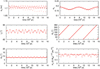 |
Fig. 8 Orbital dynamics of Kepler-419c using the elements listed in Table 1 as initial conditions. |
| In the text | |
|
Fig. 9 Long-term evolution of the semimajor axis, the eccentricity and the inclination of Kepler-419b, using the elements listed in Table 1 as initial conditions. |
| In the text | |
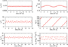 |
Fig. 10 Orbital dynamics of Kepler-419b using the elements listed in Table 1 as initial conditions. |
| In the text | |
|
Fig. 11 pb vs. qb (red dots), pc vs. qc (green dots),and pbc vs. qbc (blue dots). |
| In the text | |
|
Fig. 12 Qb (red dots) and qc (blue dots) as a function of time, for an unstable system. |
| In the text | |
|
Fig. B.1 The standard system of reference. |
| In the text | |
|
Fig. B.2 Winn’s system of reference. |
| In the text | |
|
Fig. B.3 System of reference used in D14. |
| In the text | |
Current usage metrics show cumulative count of Article Views (full-text article views including HTML views, PDF and ePub downloads, according to the available data) and Abstracts Views on Vision4Press platform.
Data correspond to usage on the plateform after 2015. The current usage metrics is available 48-96 hours after online publication and is updated daily on week days.
Initial download of the metrics may take a while.