| Issue |
A&A
Volume 620, December 2018
|
|
|---|---|---|
| Article Number | A80 | |
| Number of page(s) | 12 | |
| Section | Interstellar and circumstellar matter | |
| DOI | https://doi.org/10.1051/0004-6361/201731955 | |
| Published online | 30 November 2018 | |
ALMA observations of the young protostellar system Barnard 1b: Signatures of an incipient hot corino in B1b-S★
1
Instituto de Física Fundamental, CSIC, C/ Serrano 123,
28006
Madrid, Spain
e-mail: nuria.marcelino@csic.es
2
Sorbonne Université, Observatoire de Paris, Université PSL, École normale supérieure, CNRS, LERMA,
75014
Paris,
France
3
Observatorio Astronómico Nacional (OAN, IGN), Apdo 112,
28803
Alcalá de Henares, Spain
4
National Radio Astronomy Observatory,
520 Edgemont Road,
Charlottesville,
VA 22903, USA
5
Institut de Radioastronomie Millimétrique (IRAM),
300 rue de la Piscine,
38406 Saint Martin d’Hères,
France
6
Laboratoire d’astrophysique de Bordeaux, Univ. Bordeaux, CNRS, B18N, allée Geoffroy Saint-Hilaire,
33615 Pessac,
France
7
Sorbonne Université, Observatoire de Paris, Université PSL, CNRS, LERMA,
92190
Meudon,
France
8
Univ. Lyon, ENS de Lyon, Univ. Lyon1, CNRS, Centre de Recherche Astrophysique de Lyon UMR5574,
69007
Lyon,
France
Received:
14
September
2017
Accepted:
17
September
2018
The Barnard 1b core shows signatures of being at the earliest stages of low-mass star formation, with two extremely young and deeply embedded proto-stellar objects. Hence, this core is an ideal target to study the structure and chemistry of the first objects formed in the collapse of prestellar cores. We present ALMA Band 6 spectral line observations at ~0.6″ of angular resolution towards Barnard 1b. We have extracted the spectra towards both protostars, and used a local thermodynamic equilibrium (LTE) model to reproduce the observed line profiles. B1b-S shows rich and complex spectra, with emission from high energy transitions of complex molecules, such as CH3OCOH and CH3CHO, including vibrational level transitions. We have tentatively detected for the first time in this source emission from NH2CN, NH2CHO, CH3CH2OH, CH2OHCHO, CH3CH2OCOH and both aGg′ and gGg′ conformers of (CH2OH)2. This is the first detection of ethyl formate (CH3CH2OCOH) towards a low-mass star forming region. On the other hand, the spectra of the FHSC candidate B1b-N are free of COMs emission. In order to fit the observed line profiles in B1b-S, we used a source model with two components: an inner hot and compact component (200 K, 0.35″) and an outer and colder one (60 K, 0.6″). The resulting COM abundances in B1b-S range from 10−13 for NH2CN and NH2CHO, up to 10−9 for CH3OCOH. Our ALMA Band 6 observations reveal the presence of a compact and hot component in B1b-S, with moderate abundances of complex organics. These results indicate that a hot corino is being formed in this very young Class 0 source.
Key words: astrochemistry / ISM: clouds / ISM: individual objects: Barnard 1b / ISM: abundances / stars: formation / stars: low-mass
The full Table B.2 is only available at the CDS via anonymous ftp to cdsarc.u-strasbg.fr (130.79.128.5) or via http://cdsarc.u-strasbg.fr/viz-bin/qcat?J/A+A/620/A80
© ESO 2018
1 Introduction
In the innermost regions of low-mass Class 0 objects, gas and dust can reach temperatures of >100 K, at which water and other grain mantle components can evaporate into the gas phase. In particular, the large contribution of complex organic molecules (COMs; defined as species with six or more atoms) to their spectra, makes them similar to hot cores in massive star forming regions, and they are therefore known as hot corinos (Herbst & van Dishoeck 2009; Caselli & Ceccarelli 2012). These regions have small sizes, of <100 au, and their study has greatly improved in the last few years thanks to interferometers operating at millimetre and sub-millimetre wavelengths such as NOEMA and ALMA. In particular, ALMA observations at unprecedent angular resolution, have allowed us to probe the inner hot regions of low-mass protostars and compare with sophisticated MHD models (see, e.g. Commerçon et al. 2012; Hincelin et al. 2016).
Of particular interest are the earliest stages of low-mass star formation: the initial collapse, the formation of accretion disks and the launching of protostellar outflows. The Barnard 1 cloud is a moderately active star forming region in the Perseus molecular complex, at a distance of 230 pc (Hirota et al. 2008). It contains several dense cores at different stages of star formation, two of them, B1a and B1c, hosting class 0 sources associated with high velocity outflows (Hatchell et al. 2005, 2007). The proto-stellar core B1b contains three remarkable sources: the infrared source B1b-W, also observed recently at millimetre and sub-millimetre wavelengths (Gerin et al. 2017; Cox et al. 2018), and two extremely young protostellar objects, B1b-N and B1b-S. These two sources have been suggested to be first hydrostatic core (FHSC) candidates, which is the first object to be formed in the collapse of a prestellar core (Larson 1969). Therefore, this core has been a target of multiple studies (see, e.g. Pezzuto et al. 2012; Hirano & Liu 2014). Recent interferometric observations with NOEMA and ALMA have shown the incipient star formation activity in B1b. Gerin et al. (2015) observed young and slow outflows driven by both sources, and obtained outflow properties consistent with B1b-S being a very early Class 0 and B1b-N a FHSC candidate. ALMA continuum emission at 350 GHz at a very high resolution (0.1″), indicates the presence of small compact structures that were interpreted as nascent disks by Gerin et al. (2017). Using NOEMA at ~ 4″, Fuente et al. (2017) imaged the emission of NH2D, which is tracing the pseudo-disk, and detected rotation around B1b-S. Here we present spectral line ALMA observations at 0.6″ angular resolution of the two young proto-stars B1b-N and B1b-S.
2 Observations
ALMA Cycle 3 observations were performed on 2016 June 21–24, in four different tracks of about an hour each. The ALMA 12 m array was used in the C40-4 configuration, with 36–40 antennas and baselines between 15.1 and 704.1 m. The mean angular resolution achieved (interferometric synthesised beam) at the observed frequencies is ~0.7 × 0.55″ (160 × 126 au), and the largest scales to which we are sensitive are ~4″. We used the Band 6 receiver centred at 218 and 233 GHz in the lower and upper side band, respectively, connected to the ALMA correlator in FDM mode. In total, 13 spectral windows were used, one at low resolution (~40 km s−1 and 2 GHz of bandwidth) for the continuum, and 12 windows with spectral resolutions of ~0.16–0.2 km s−1 and a 58.5 MHz bandwidth.
We performed a seven-point mosaic centred at αJ2000 = 03h33m21.3s and δJ2000 = 31°07′34.0″, covering an area of 40 arcsec2 containing B1b-N, B1b-S, and the infrared source B1b-W. All the fields were observed in scans of approximately seven minutes duration, with 30 s scans for phase calibration in-between. Total time on-source is 44 min per track. The phase calibrator used is J0336+3218, located at a distance of ~1.36° of the B1b cores. Two other quasars were observed for bandpass (J0237+2848) and flux (J0238+1636) calibration. Flux density for J0238+1636 was set to ~1.14–1.22 Jy, depending on the day and frequency, based on close flux measurements. Calibration was performed by the ALMA Pipeline in CASA1 4.5.3. Images of all spectral windows were also produced in CASA, with a spectral resolution of 0.2 km s−1 and Briggs weighting. Table B.1 gives the frequency ranges, the final beam and rms of the images. For analysis purposes we used the GILDAS2 software. We have extracted the spectra, within one synthesised beam size, towards the positions of the B1b-N and B1b-S cores. Depending on the frequency and the beam for each spectral window, we have converted the flux into brightness temperature to analyse the spectra (K Jy−1 ~ 63).
3 Results
The obtained spectra towards the two sources look very different: while B1b-S shows intense and rich spectra, B1b-N is mostly free of line emission. The right-hand panels in Fig. 1 show one of the observed spectral windows, between 215 810 and 215 870 MHz, towards B1b-N (top) and B1b-S (bottom), and Figs. B.1–B.3 present the full spectral coverage. In the northern source, we observe lines from 12CO, 13CO, C18 O, 13CS, DCO+, DCN, N2 D+, and SO. All of them show extended emission and towards the position of the protostar present complex line profiles, which in some cases are only seen in absorption (e.g. 12CO, and SO). One transition of H2 C17O is marginally detected in emission. All these species are also observed in B1b-S, together with lines from H2 CO, H CO, D2 CO, CH3 OH, 13CH3OH, CH2 DOH, CH3 OD and several COMs. In total, we have detected 190 lines towards B1b-S. Of those, 113 spectral features have been assigned to 155 transitions from 36 species (including isotopologues and vibrational states). Table B.2 lists all assigned transitions and their associated species in B1b-S, with line parameters obtained from Gaussian line fits. Line identification was carried out using MADEX3 (Cernicharo 2012). The other 77 lines for which we could not find reasonable carriers are labeled as unidentified (~40% of the total number of lines). Of those, 16 have also been observed in Orion KL, that is only 21% of the unidentified lines. All transitions listed in Table B.2 are above the 3σ level (with
  , Dv the linewidth, and dv the spectral resolution), while U lines were considered above 4σ. Several lines, mainly from the most abundant species and low energy transitions, show extended emission when looking at the maps and present complex line profiles towards the position of B1b-S (lines in absorption, inverse P Cygni profiles, line wings, etc.). These lines are indicated in Table B.2 by CP or Ext (for complex profile and extended, respectively), and we do not include them in the analysis below. While we have identified all the lines in the observed spectra (see Figs. B.1–B.3 and Table B.2), the analysis of the extended emission is outside the scope of this paper. Furthermore, it is likely that a significant fraction of the flux is resolved out in the ALMA 12 m-array observations.
In the following we focus on the emission from COMs in the protostar B1b-S. We have detected multiple transitions of acetaldehyde (CH3 CHO) and methyl formate (CH3OCOH), including emission from their deuterated substitutions and vibrational states. We have also observed emission from isocyanic acid (HNCO), cyanamide (NH2 CN), formamide (NH2 CHO), vinyl cyanide (CH2 CHCN), propenal (t-CH2CHCHO), ethanol (t-CH3CH2OH), dimethyl ether (CH3 OCH3), ethyl formate (t-CH3CH2OCOH), glycolaldehyde (CH2OHCHO) and both aGg′ and gGg′ conformers of ethylene glycol ((CH2OH)2). However, some of these should be considered tentative detections. In particular, we have detected only one unblended line of HNCO, NH2 CN, NH2 CHO, t-CH2CHCHO, CH2 OHCHO, t-CH3CH2OH, and CH3 OCH3. Of the 16 transitions observed from the ethylene glycol conformers, 8 are blended with transitions from other species. We clearly detect three unblended lines from CH3 CH2OCOH, which has only been previously detected towards Sgr B2, Orion KL, and the hot core in W51 (Belloche et al. 2009; Tercero et al. 2013; Rivilla et al. 2017). We would like to point out the large number of unassigned lines and the high level of blending and complexity in the spectra (see Figs. B.1–B.3 and Table B.2), similar to that observed typically in hot cores and hot corinos. The emission of all these complex species is unresolved in the ALMA images. We have checked that at one beam separation from the position of the B1b-S protostar the spectra are free of COMs emission.
4 Column densities and abundances
We have used MADEX (Cernicharo 2012) to reproduce the observed spectra of COMs in B1b-S, and to obtain column densities and kinetic temperatures of the emitting region. We assumed local thermodynamic equilibrium (LTE) conditions, since the densities at the centre of the core are expected to be very high (Gerin et al. 2017). We have focused on CH3OCOH and CH3CHO, and their isotopic substitutions and vibrationally excited states, for which many transitions are available, to obtain the source model which was then used for the other observed species.
Methyl formate is the species for which the largest number of transitions were identified. In total 24 transitions from both A and E species were observed (18 unblended), with energy levels between 100 and 500 K, allowing to constrain the properties of the emitting region from the LTE model. We ran a set of models using one source component of 0.6″ in size (the angularresolution of the ALMA band 6 observations), and we modified the temperature and column density to fit the observed spectra. However, it was difficult to fit all the lines with only one component. The problem became more evident when using the deuterated substitutions, CH3OCOD and CH2DOCOH, and the vibrationally excited states νt = 1 and νt = 2. We have detected 12 transitions from CH3OCOD and four transitions from CH2DOCOH (three and two, respectively, are blended with other species), with upper energy levels between 90 and 170 K. In both cases the model gave better results when decreasing the temperature with respect to the best CH3OCOH model. On the other hand, the vibrationally excited lines (13 unblended transitions from νt = 1, and one transition from νt = 2), supported the high temperature model. Therefore, we built a model of the source with two components. One warm and compact component at 200 K and a size of 0.35″ (that of the continuum compact emission obtained by ALMA Band 7 observations, Gerin et al. 2017), and another larger (0.6″, approximately the angular resolution of the Band 6 observations) and colder component at 60 K. Figure B.4 shows two examples of the best one component models obtained using the main CH3OCOH (200 K), and the deuterated methyl formate lines (60 K), together with the final two component model. While some species give reasonable agreement with observations using either model (mostly those which observed transitions have similar energy levels), there are others (besides the ones discussed above) that fail in one of the models (e.g. HNCO and t-CH3CH2OCOH). We have checked that using other temperatures (between 50 and 250 K) in the one component models does not reproduce satisfactorily the observations. For the vibrationally excited states, we only used the compact component at 200 K, since the low temperature one does not contribute much to the line intensities. Indeed, energy levels of the observed transitions range between 300 and 500 K, supporting this scenario. We have also observed five transitions of 13CH3OCOH, with energies ≤200 K and intensities of the order of 500 mK or below. Since the lines are weak, any of the models give reasonable agreement with the observations. Acetaldehyde is the other species for which many lines are observed. We have detected 15 transitions (10 unblended) from the main species, with energies between 100 and 300 K. We have also detected one transition arising from the deuterated substitution CH3CDO, and four transitions (two of them blended) from the vibrational state νt = 1, with energy levels of ~300–400 K. We used the same model as methyl formate, except for CH3CHO νt = 1, for which only the compact and hot component was considered. The model allows to reproduce all transitions reasonably well, except for a few lines that are overestimated: two CH3OCOH transitions (Fig. B.1, second panel), three CH3OCOH νt = 1 lines (top panel in Fig. B.1, and second panel in Fig. B.3), and two lines from CH3CHO (see Fig. B.3, second and third panels). These are transitions with the lowest energies (~100 K) and the highest line strengths and Einstein coefficients, and may consequently have high opacities. We estimate the error in the fit to be ~50%.
This simple two-component model simulates the temperature gradient that should exist in the source. It is possible that a more sophisticated model will reproduce the lines better, however the limited angular resolution and signal-to-noise ratio of the current observations do not allow a well-constrained model. In particular, the angular resolution is not sufficient to separate the emission from the compact and hot component at 200 K from that of the lukewarm gas at 60 K. For example, it is possible that the size of the hot component could be smaller, and therefore we underestimate the column densities.
For the other COMs, we have used the same two-component model as for methyl formate and acetaldehyde for consistency. There are two exceptions: the observed lines from 13CH3OH and HNCO arise from very excited energy levels (~ 600 and 700 K, respectively). Hence, we have assumed that only the hot and compact component contributes to the detected emission. As mentioned above, we have excluded from the analysis all the species with lines showing complex profiles and extended emission. We have attempted to run the LTE models for CH3OH, H2 CO and their isotopologues, which do not show absorption or very complex profiles. All the observed lines of H2 CO, H CO, H2 C17O, and D2 CO (only one transition each) have low Eup values and show extended emission. Therefore, these lines will suffer from flux loss due to filtering from the interferometer, and the obtained column densities are strongly underestimated. For CH3OH and CH2DOH we observed more than one transition (two and six, respectively), but they span a considerable Eup range, which makes a simultaneous fit difficult. In particular, lines with low energies and extended emission are significantly overestimated. We have observed only one transition from CH3OD (also extended) and 13CH3OH. We have kept only the LTE result for the latter which does not present any extended emission. Lines from DCO+, DCN, C18 O, SO, 13CO, CO, 13CS, and N2 D+, are seen in absorption or show very complex profiles, and we have not attempted to fit them with the LTE model. For all these species, we show the line identification in Figs. 1 and B.1–B.3.
Table 1 shows, for each source component, the obtained column densities and molecular abundances with respect to H2. In order to compute the abundances we have estimated the molecular hydrogen column densities for both components. Based on previous observations of dust continuum emission with ALMA at 850 μm and JVLA at 8–10 cm (those with the best angular resolution, see Appendix A) and assuming dust temperatures from 12 to 50 K, we have computed mean column densities of N(H2) = 1.4 × 1025 cm−2 and 1.1 × 1025 cm−2 for source sizes of 0.35″ and 0.6″, respectively.While the dust emission is optically thick at 350 GHz on size scales smaller than 0.3″, the 8 cm emission is optically thin. Then it is possible the H2 column density estimates could be affected by the opacity, in particular at 0.35′′ more than at 0.6′′. Another important source of error comes from the unknown dust properties, since the standard opacity law may be different if dust grains have grown. All these factors could result in uncertainties in the column density estimates up to a factor of two.
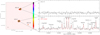 |
Fig. 1 Left panel: Continuum image at 232 GHz (1.290 mm). The colour scale ranges from 0.001 to 0.2 Jy beam−1. The contour levels are indicated on the colour bar. The ALMA beam is plotted on the lower left corner. Right panel: Observed spectra between 215 810 and 215 870 MHz, towards B1b-N (top panel) and B1b-S (bottom panel). Brightness temperaturescale, in K, is given on the left. Line features with no labels are unidentified lines. The LTE simulations are over-plotted in red for B1b-S. |
Results from LTE model.
5 Discussion
Previous spectral studies with the IRAM 30 m telescope already pointed out the presence of complex organics in B1b. Cernicharo et al. (2012) reported the detection of several COMs, including CH3CHO, CH3OCOH, and CH3OCH3, also observed with ALMA. These detections are based on low energy transitions, <25 K, and because of the large 30 m beam at 3 mm (30−21″) the emission should be arising from the cold envelope. Table B.3 shows the abundances derived from the ALMA data, together with those obtained in the envelope from the IRAM 30 m survey at 3 mm. Except for CH2CHCN and HNCO, there is a general trend of COMs being enhanced in the inner core of B1b-S with respect to the colder protostellar envelope, with methyl formate showing the highest increase. This may be related to the evaporation of grain mantles due to the increased dust temperature caused by the heating from the embedded protostar. A similar increase in abundance is seen in other hot corinos with respect to the values observed in their envelopes. In IRAS 16293-2422, Jaber et al. (2014) obtain higher abundances in the inner warm envelope with respect to the outer cold envelope, and these values are lower than those observed at smaller scales using interferometers, in other words, closer to the proto-star (Jørgensen et al. 2012; Coutens et al. 2018). The range of temperatures obtained for B1b-S cores in the LTE model, from 60 K up to at least 200 K in a size of 0.35′′, and the narrow line-widths are consistent with thermal evaporation. Other mechanisms could also be at work, such as accretion shocks in the disk or launching of the outflow. However, we can not conclude about the origin of COMs since we lack angular resolution. Indeed, it is possible that the size of the compact component in the model (0.35′′) is smaller, since we do not resolve the emission from the highest energy transitions.
In the ALMA data we have also detected the singly deuterated isotopologues of acetaldehyde and methyl formate, whose abundances decrease at the inner hot component with respect to the component at 60 K, with D/H a factor of five higher in the latter (see Table B.3). These deuterated species are not detected with the IRAM 30 m, possibly because the main species are weak and less abundant in the envelope. However, high deuteration levels are observed for other species, for example, strong HDCO lines were detected by Marcelino et al. (2005) with a D to H ratio of 0.145. This value is similar to those derived in the external B1b-S core for CH3OCOD and CH2DOCOH (D/H of 0.1 and 0.2, respectively), and smaller than CH3CDO/CH3CHO = 0.25. High deuterium fractionation is also observed in hot corinos, while hot cores show lower deuterium abundances (see Caselli & Ceccarelli 2012, and references within).
The comparison with other hot corinos is not easy since we have a limited number of lines, in contrast to well-known sources that have been more extensively observed with ALMA and NOEMA, such as IRAS 16293-2422 (Jørgensen et al. 2016), NGC1333 IRAS 2A and 4A (Taquet et al. 2015; López-Sepulcre et al. 2017). In general, we find a similar inventory ofCOMs but with lower abundances in B1b-S. We are going to discuss only some trends and ratios between them. For example, one similarity with hot corinos are the higher abundances of O-bearing COMs with respect to N-bearing COMs. We observe a similar trend in B1b-S, where the highest abundances are obtained for CH3OCOH, CH3OCH3, and CH3CHO, while NH2CN and NH2CHO show the lowest abundances. Cyanamide has been recently detected towards the low-mass protostars IRAS 16293-2422 and NGC 1333 IRAS2A (Coutens et al. 2018), with observed NH2CN to NH2CHO ratios of 0.2and 0.02, respectively. These values are in the range of those observed towards the molecular clouds in the Galactic centre but lower than in Orion KL (Coutens et al. 2018). We obtain in B1b-S anabundance ratio of 0.25, similar to IRAS 16293-2422. Of the three possible isomers of C2 H4O2, we have detected CH3OCOH and CH2OHCHO. The observed CH3OCOH to CH2OHCHO ratio in B1b-S, ~20, is similar to that observed in the low-mass protostars in NGC 1333 and IRAS 16293-2422 (Taquet et al. 2015; Jørgensen et al. 2012). Acetic acid (CH3COOH) is the most stable but the least abundant of the three isomers (Lattelais et al. 2010). It has been observed in IRAS 16293-2422 with a ratio with respect to glycolaldehyde of ~11 (Jørgensen et al. 2016), consistent with the 5–15 upper limits in B1b-S. Glycolaldehyde and its corresponding alcohol, ethylene glycol, show similar abundances in B1b-S, slightly higher for CH2OHCHO. This is in contrast to other hot cores and hot corinos (Fuente et al. 2014; Jørgensen et al. 2016; Favre et al. 2017). However, since detections of these species are based on just a few lines, in particular for glycolaldehyde, column densities may be not well constrained and it is difficult to make definite conclusions. We have detected CH3CH2OCOH for the first time in a low-mass protostar, with a relatively high abundance of 10−11. This detection shows that the molecular complexity is high in young hot corinos and other species with a larger number of atoms could be present. It is noteworthy that this species has not been previously observed in the well-known hot corinos IRAS 16293-2422 and NGC 133IRAS4A. We have checked in the ALMA spectral line survey of IRAS 16293-2422 (PILS, Jørgensen et al. 2016), and no clear features are seen, although the observed frequencies are different. It is possible that the high level of line confusion and wide linewidths prevent the detection of weak lines in these more evolved sources.
Observed line widths in B1b-S are typically narrow, ~1 km s−1 (see Table B.2), in contrast to the wide line profiles in hot cores and hot corinos (~3–5 km s−1). Besides all lines from COMs are found in emission, with no P Cygni or absorption profiles. Therefore, there is no signature of rotation or infall in the disk or core from COMs. The orientation of the disk should not prevent the detection of rotation, following the observations of the outflows in B1b-S (Gerin et al. 2015). Actually, using NOEMA data, Fuente et al. (2017) detect rotation using NH2D. The absence of detected rotation could be due to the too low angular resolution since the COM emission is unresolved. In addition, although the sensitivity is excellent, these observations are not deep enough to detect weak features at the 0.3–0.6 K level (see rms in Table B.1). Hence, weak line wings with rotation signatures may have been missed.
6 Conclusions
We present new ALMA Band 6 data towards the protostellar system B1b in Perseus. We have detected a rich and complex spectra in B1b-S, with 190 spectral features. Of those, 99 lines are assigned to transitions from complex molecules, while 77 remain unidentified. Previous NOEMA observations do not show any emission from COMs, with spatial resolutions between 2″ and 5″ (Gerin et al. 2015; Fuente et al. 2017). These data suggest that embedded in the B1b-S core a very young and compact object is already warming up its most immediate surroundings, where molecules from grain mantles are evaporating. On the other hand, B1b-N is almost free of line emission. The non-detection of complex species supports the scenario in which B1b-N is at an earlier stage of evolution than B1b-S. Another possibility is that the more active outflow in B1b-S, with higher velocities and more complex profiles (with evidences of bullets), could contribute to a more efficient release of COM in the gas phase in B1b-S, as compared to B1b-N. Luminosity outbursts due to episodic accretion in B1b-S could also increase the dust temperatureand produce the evaporation of COMs from grain mantles or trigger the formation of daughter molecules in the gas phase (Taquet et al. 2016). The origin of COMs in B1b-S remains unclear since the emission is not resolved.
While B1b-S presents a rich spectra similar to other hot corinos, observed line widths are typically narrower and do not show any signature of rotation or infall. This could be due to the limited angular resolution and signal-to-noise ratio. These observations confirm that hot corinos are a common feature in class 0 protostars, but require sub-arcsec angular resolution and high sensitivity reaching a few mJy beam−1 to be detected. Higher angular resolution observations of B1b-S with better sensitivity are desirable to resolve the emission from COMs, and better constrain molecular abundances, the size and the structure of the emitting region.
Acknowledgements
We thank the referee for a careful reading of the manuscript and useful comments which have improved the paper significantly. This paper makes use of the following ALMA data: ADS/JAO.ALMA#2015.1.00025.S. ALMA is a partnership of ESO (representing its member states), NSF (USA) and NINS (Japan), together with NRC (Canada), MOST and ASIAA (Taiwan), and KASI (Republic of Korea), in cooperation with the Republic of Chile. The Joint ALMA Observatory is operated by ESO, AUI/NRAO and NAOJ. We acknowledge funding support from the European Research Council (ERC Grant 610256: NANOCOSMOS), the ANR project IMOLABS, and the Spanish MINECO under projects AYA2016-75066-C2-2-P and AYA2012-32032. This work was partly supported by the Programme National “Physique et Chimie du Milieu Interstellaire” (PCMI) of CNRS/INSU with INC/INP, co-funded by CEA and CNES. The National Radio Astronomy Observatory is a facility of the National Science Foundation operated under cooperative agreement by Associated Universities, Inc.
Appendix A Continuum results
The frequency setup included a broad spectral window, in order to detect the continuum emission of the B1b sources, andto facilitate the bandpass and phase calibration on the reference quasars. We present in the left panel in Fig. 1 the resulting continuum image. The three Barnard 1b protostars are detected, B1b-N, B1b-S and even the weak source B1b-W. Table A.1 provides a compilation of the spectral energy distribution for these three sources. Given the extended nature of the sources the listed values depend on the angular resolution of the observations. It is therefore important to compare data measured at the same angular resolution.
Observed fluxes at different wavelengths for the B1b sources.
Appendix B Additional figures and tables
Summary of the observed spectral line windows.
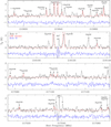 |
Fig. B.1 Observed spectra towards B1b-S (black) and B1b-N (blue), between 215810 and 217268 MHz. Line features with no labels are unidentified lines. The LTE simulations for B1b-S are over-plotted in red. |
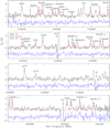 |
Fig. B.2 Observed spectra towards B1b-S (black) and B1b-N (blue), between 218432 and 220426 MHz. Line features with no labels are unidentified lines. The LTE simulations for B1b-S are over-plotted in red. |
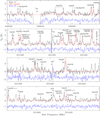 |
Fig. B.3 Observed spectra towards B1b-S (black) and B1b-N (blue), between 230519 and 231440 MHz. Line features with no labels are unidentified lines. The LTE simulations for B1b-S are over-plotted in red. |
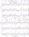 |
Fig. B.4 Best LTE models using only one source component for two spectral windows. Middle panels for each frequency range show the results for the 200 K model in red, while bottom panels show in blue the 60 K model. Top panels in purple show the final two-component model. |
Observed transitions in B1b-S.
Obtained abundances with respect to H2 in B1b-S (this work), and towards the B1b envelope observed with the IRAM 30 m. The D/H obtained for acetaldehyde and methyl formate for the hot and cold components in B1b-S are also shown.
References
- Belloche, A., Garrod, R. T., Müller, H. S. P., et al. 2009, A&A, 499, 215 [NASA ADS] [CrossRef] [EDP Sciences] [Google Scholar]
- Caselli, P., & Ceccarelli, C. 2012, A&ARv, 20, 56 [NASA ADS] [CrossRef] [MathSciNet] [Google Scholar]
- Cernicharo, J. 2012, in ECLA-2011: Proc. of the European Conference on Laboratory Astrophysics, EAS Pub. Ser., eds. C. Stehlé, C. Joblin, & L. d’Hendecourt (Cambridge: Cambridge Univ. Press) [Google Scholar]
- Cernicharo, J., Marcelino, N., Roueff, E., et al. 2012, ApJ, 759, L43 [NASA ADS] [CrossRef] [Google Scholar]
- Commerçon, B., Levrier, F., Maury, A. J., Henning, Th., & Launhardt, R. 2012, A&A, 548, A39 [NASA ADS] [CrossRef] [EDP Sciences] [Google Scholar]
- Coutens, A., Willis, E. R., Garrod, R. T., et al. 2018, A&A, 612, A107 [NASA ADS] [CrossRef] [EDP Sciences] [Google Scholar]
- Cox, E. G., Harris, R. J., Looney, L. W., et al. 2018, ApJ, 855, 92 [NASA ADS] [CrossRef] [Google Scholar]
- Daniel, F., Gerin, M., Roueff, E., et al. 2013, A&A, 560, A3 [NASA ADS] [CrossRef] [EDP Sciences] [Google Scholar]
- Evans, N. J., II, Dunham, M. M., J orgensen, J. K., et al. 2009, ApJS, 181, 321 [NASA ADS] [CrossRef] [Google Scholar]
- Favre, C., Pagani, L., Goldsmith, P., et al. 2017, A&A, 604, L2 [NASA ADS] [CrossRef] [EDP Sciences] [Google Scholar]
- Fuente, A., Cernicharo, J., Caselli, P., et al. 2014, A&A, 568, A65 [NASA ADS] [CrossRef] [EDP Sciences] [Google Scholar]
- Fuente, A., Gerin, M., Pety, J., et al. 2017, A&A, 606, L3 [NASA ADS] [CrossRef] [EDP Sciences] [Google Scholar]
- Gerin, M., Pety, J., Fuente, A., et al. 2015, A&A, 577, L2 [NASA ADS] [CrossRef] [EDP Sciences] [Google Scholar]
- Gerin, M., Pety, J., Commerçon, B., et al. 2017, A&A, 606, A35 [NASA ADS] [CrossRef] [EDP Sciences] [Google Scholar]
- Hatchell, J., Richer, J. S., Fuller, G. A., et al. 2005, A&A, 440, 151 [NASA ADS] [CrossRef] [EDP Sciences] [Google Scholar]
- Hatchell, J., Fuller, G. A., & Richer, J. S. 2007, A&A, 472, 187 [NASA ADS] [CrossRef] [EDP Sciences] [Google Scholar]
- Herbst, E., & van Dishoeck, E. F. 2009, ARA&A, 47, 427 [NASA ADS] [CrossRef] [Google Scholar]
- Hincelin, U., Commerçon, B., Wakelam, V., et al. 2016, ApJ, 822, 12 [NASA ADS] [CrossRef] [Google Scholar]
- Hirano, N., & Liu, F. -C. 2014, ApJ, 789, 50 [NASA ADS] [CrossRef] [Google Scholar]
- Hirota, T., Bushimata, T., Choi, Y. K., et al. 2008, PASJ, 60, 37 [NASA ADS] [CrossRef] [Google Scholar]
- Jaber, A. A., Ceccarelli, C., Kahane, C., & Caux, E. 2014, ApJ, 791, 29 [Google Scholar]
- Jørgensen, J. K., Favre, C., Bisschop, S. E., et al. 2012, ApJ, 757, L4 [NASA ADS] [CrossRef] [Google Scholar]
- Jørgensen, J. K., van der Wiel, M. H. D., Coutens, A., et al. 2016, A&A, 595, A117 [NASA ADS] [CrossRef] [EDP Sciences] [Google Scholar]
- Larson, R. B. 1969, MNRAS, 145, 271 [NASA ADS] [CrossRef] [Google Scholar]
- Lattelais, M., Pauzat, F., Ellinger, Y., & Ceccarelli, C. 2010, A&A, 519, A30 [NASA ADS] [CrossRef] [EDP Sciences] [Google Scholar]
- López-Sepulcre, A., Sakai, N., Neri, R., et al. 2017, A&A, 606, A121 [NASA ADS] [CrossRef] [EDP Sciences] [Google Scholar]
- Marcelino, N., Cernicharo, J., Roueff, E., et al. 2005, ApJ, 620, 308 [NASA ADS] [CrossRef] [Google Scholar]
- Marcelino, N., Cernicharo, J., Tercero, B., & Roueff, E. 2009, ApJ, 690, L27 [NASA ADS] [CrossRef] [Google Scholar]
- Pezzuto, S., Elia, D., Schisano, E., et al. 2012, A&A, 547, A54 [NASA ADS] [CrossRef] [EDP Sciences] [Google Scholar]
- Pokhrel, R., Myers, P. C., Dunham, M. M., et al. 2018, ApJ, 853, 5 [NASA ADS] [CrossRef] [Google Scholar]
- Rivilla, V. M., Beltrán, M. T., Martín-Pintado, J., et al. 2017, A&A, 599, A26 [NASA ADS] [CrossRef] [EDP Sciences] [Google Scholar]
- Taquet, V., López-Sepulcre, A., Ceccarelli, C., et al. 2015, ApJ, 804, 81 [NASA ADS] [CrossRef] [Google Scholar]
- Taquet, V., Wirström, E. S., & Charnley, S. B. 2016, ApJ, 821, 46 [NASA ADS] [CrossRef] [Google Scholar]
- Tercero, B., Kleiner, I., Cernicharo, J., et al. 2013, ApJ, 770, L13 [Google Scholar]
- Tobin, J. J., Looney, L. W., Li, Z.-Y., et al. 2016, ApJ, 818, 73 [NASA ADS] [CrossRef] [Google Scholar]
All Tables
Obtained abundances with respect to H2 in B1b-S (this work), and towards the B1b envelope observed with the IRAM 30 m. The D/H obtained for acetaldehyde and methyl formate for the hot and cold components in B1b-S are also shown.
All Figures
|
Fig. 1 Left panel: Continuum image at 232 GHz (1.290 mm). The colour scale ranges from 0.001 to 0.2 Jy beam−1. The contour levels are indicated on the colour bar. The ALMA beam is plotted on the lower left corner. Right panel: Observed spectra between 215 810 and 215 870 MHz, towards B1b-N (top panel) and B1b-S (bottom panel). Brightness temperaturescale, in K, is given on the left. Line features with no labels are unidentified lines. The LTE simulations are over-plotted in red for B1b-S. |
| In the text | |
|
Fig. B.1 Observed spectra towards B1b-S (black) and B1b-N (blue), between 215810 and 217268 MHz. Line features with no labels are unidentified lines. The LTE simulations for B1b-S are over-plotted in red. |
| In the text | |
|
Fig. B.2 Observed spectra towards B1b-S (black) and B1b-N (blue), between 218432 and 220426 MHz. Line features with no labels are unidentified lines. The LTE simulations for B1b-S are over-plotted in red. |
| In the text | |
|
Fig. B.3 Observed spectra towards B1b-S (black) and B1b-N (blue), between 230519 and 231440 MHz. Line features with no labels are unidentified lines. The LTE simulations for B1b-S are over-plotted in red. |
| In the text | |
|
Fig. B.4 Best LTE models using only one source component for two spectral windows. Middle panels for each frequency range show the results for the 200 K model in red, while bottom panels show in blue the 60 K model. Top panels in purple show the final two-component model. |
| In the text | |
Current usage metrics show cumulative count of Article Views (full-text article views including HTML views, PDF and ePub downloads, according to the available data) and Abstracts Views on Vision4Press platform.
Data correspond to usage on the plateform after 2015. The current usage metrics is available 48-96 hours after online publication and is updated daily on week days.
Initial download of the metrics may take a while.