| Issue |
A&A
Volume 619, November 2018
|
|
|---|---|---|
| Article Number | A106 | |
| Number of page(s) | 9 | |
| Section | Galactic structure, stellar clusters and populations | |
| DOI | https://doi.org/10.1051/0004-6361/201833901 | |
| Published online | 14 November 2018 | |
3D shape of Orion A from Gaia DR2⋆
1
Universität Wien, Institut für Astrophysik, Türkenschanzstrasse 17, 1180 Wien, Austria
e-mail: This email address is being protected from spambots. You need JavaScript enabled to view it.
2
University of Vienna, Research Platform, Data Science @ Uni Vienna, Austria
3
Universidade do Porto, Departamento de Engenharia Física da Faculdade de Engenharia, Rua Dr. Roberto Frias, 4200-465 Porto, Portugal
4
Laboratoire d’Astrophysique de Bordeaux, Université de Bordeaux, Allée Geoffroy Saint-Hilaire, CS 50023, 33615 Pessac Cedex, France
5
Universitäts-Sternwarte Ludwig-Maximilians-Universität (USM), Scheinerstr. 1, 81679 München, Germany
6
Max-Planck-Fellow, Max-Planck-Institut für extraterrestrische Physik (MPE), Giessenbachstr. 1, 85748 Garching, Germany
7
Centre for Astrophysics Research, University of Hertfordshire, College Lane, Hatfield, AL10 9AB, UK
8
Harvard-Smithsonian Center for Astrophysics, 60 Garden Street, Cambridge, MA, 02138, USA
9
Leiden Observatory, Niels Bohrweg 2, 2333 CA Leiden, The Netherlands
10
University of Milan, Department of Physics, via Celoria 16, 20133 Milan, Italy
11
CENTRA, Universidade de Lisboa, FCUL, Campo Grande, Edif. C8, 1749-016 Lisboa, Portugal
12
Cavendish Laboratory, University of Cambridge, 19 J.J. Thomson Avenue, Cambridge, CB3 0HE, UK
Received:
18
July
2018
Accepted:
11
August
2018
Abstract
We use the Gaia DR2 distances of about 700 mid-infrared selected young stellar objects in the benchmark giant molecular cloud Orion A to infer its 3D shape and orientation. We find that Orion A is not the fairly straight filamentary cloud that we see in (2D) projection, but instead a cometary-like cloud oriented toward the Galactic plane, with two distinct components: a denser and enhanced star-forming (bent) Head, and a lower density and star-formation quieter ∼75 pc long Tail. The true extent of Orion A is not the projected ∼40 pc but ∼90 pc, making it by far the largest molecular cloud in the local neighborhood. Its aspect ratio (∼30:1) and high column-density fraction (∼45%) make it similar to large-scale Milky Way filaments (“bones”), despite its distance to the galactic mid-plane being an order of magnitude larger than typically found for these structures.
Key words: methods: statistical / methods: observational / parallaxes / stars: distances / stars: formation / local insterstellar matter
Full Table B.1 is only available at the CDS via anonymous ftp to cdsarc.u-strasbg.fr (130.79.128.5) or via http://cdsarc.u-strasbg.fr/viz-bin/qcat?J/A+A/619/A106
© ESO 2018
1. Introduction
The archetypal giant molecular cloud (GMC) Orion A is the most active star-forming region in the local neighborhood, having spawned ∼3000 young stellar objects (YSOs) in the last few million years (e.g., Megeath et al. 2012; Furlan et al. 2016; Großschedl et al. 2018). Some of the most basic observables of the star-formation process, including star-formation rates and history, age spreads, multiplicity, the initial mass function, and protoplanetary disk populations, have been derived for this benchmark region (e.g., Bally 2008; Muench et al. 2008). Previous distance estimates to the Orion nebula cluster (ONC), the richest cluster toward the northern end of the cloud, put this object at about 400 pc from Earth (e.g., Sandstrom et al. 2007; Menten et al. 2007; Hirota et al. 2007; Kim et al. 2008; Kuhn et al. 2018). Moreover, there has been some evidence that the northern part of the cloud, including the ONC (or “Head”), is closer than the southern part (or “Tail”)1, containing L1641 and L1647 (Schlafly et al. 2014; Kounkel et al. 2017, 2018).
To know the true 3D spatial shape and orientation of this giant filamentary structure would allow one not only to determine accurate cloud and YSO masses, luminosities, and separations for this benchmark region, but it would also bring important hints on the formation of GMCs in the disk of the Milky Way. Schlafly et al. (2014) first found an indication of a distance gradient across Orion A (see Table 1), using a method based on optical reddening of stars (Green et al. 2014) which is not sensitive to regions of high column-density. Schlafly et al. found that the Tail of the cloud is about 70 pc more distant than the ONC region. Kounkel et al. (2017) conducted 15 VLBI observations toward young stars near the ONC, and two observations toward L1641-South. These observations again suggest an inclination of the cloud away from the plane of the sky, with a difference in distance of about 40 pc from Head to Tail (until L1641-South). The distances reported in Schlafly et al. (2014) and Kounkel et al. (2017) are presented in Fig. A.1 and in Table 1. Kounkel et al. (2018) continued the analysis of this region by using new APOGEE-2 data combined with the newly released Gaia DR2 catalog (Gaia Collaboration 2018b). In this recent paper, they focus on stellar populations and the star-formation history across the whole Orion complex in a high dimensional space using a clustering algorithm. They report a more distant Tail compared to the Head (about 55 pc distance difference).
Distances to sub-regions in Orion A from the literature.
In this paper we have used the newly released Gaia DR2 to infer the 3D shape and orientation of Orion A. As a proxy to the cloud distance we will use the latest catalog of mid-infrared selected YSOs in this cloud, with ages ≲3 Myr, for which a Gaia DR2 parallax measurement exists. These very young stars lie relatively close to, or are still embedded in the Orion A GMC, sharing the same velocity as the cloud (Tobin et al. 2009; Hacar et al. 2016), and are thus the best tracer of the cloud’s shape.
2. Observations and data selection
We have used the Orion A YSO catalog of Großschedl et al. (2018) which revisited the catalog of Megeath et al. (2012), including updates from Megeath et al. 2016; Furlan et al. 2016; Lewis & Lada 2016), and added about 200 new YSO candidates from a dedicated ESO-VISTA near-infrared survey covering the whole Orion A region (∼18 deg2, Meingast et al. 2016), making it the most complete (2D) distribution of YSOs toward this cloud. The catalog contains 2978 YSO candidates with IR-excess, classified into 2607 pre-main-sequence stars with disks (Class II), 183 flat-spectrum sources, and 188 protostars (Class 0/I). The on-sky distribution of these sources generally follows the high density regions of the cloud (see Fig. 3, bottom). Combined with their youth, this makes them a good proxy for cloud distances.
To infer the distance along the Orion A GMC we averaged over YSO’s parallaxes (ϖ) in equally sized bins of Galactic longitude (Δl). To derive distances from parallaxes we have investigated both the inverse of ϖ and the Bayesian distance estimates from Bailer-Jones et al. (2018), which account for the non-linearity of the transformation parallax to distance. At a distance of 400 pc, the mean difference between the two methods is about 1% for DR2, meaning that the final result in this paper will be virtually independent of the method used to infer distances. Moreover, we do not include a global parallax offset of 0.029 mas or 0.08 mas, as discussed in Lindegren et al. (2018) and Stassun & Torres (2018), since it is very uncertain how or if this effect influences the parallaxes of our sample toward Orion A. Besides, the presence of a small offset does not affect the result in this paper. To summarize, in this paper we use parallaxes when possible, and only then we derive the mean or median distance from the inverse of the mean(ϖ) or median(ϖ).
Before cross-matching the YSO sample with Gaia DR2 data we checked the effect of proper motions on the cross-match. To this end, we transformed Gaia J2015.5 coordinates into J2000. The effect toward Orion A is marginal, with a mean separation between J2015.5 and J2000 of 0.09″, smaller than the astrometric accuracy of the VISTA survey (observed in 2013). We used then a 1″ cross-match radius between the original Gaia J2015.5 and VISTA coordinates. This results in 1986 cross-matches of DR2 parallaxes with IR-excess YSOs (67% of the original YSO catalog).
Since we are interested in reliable anchor points along the cloud, and given the relatively good statistics, we chose a conservative selection criteria for the final sample (informed by Gaia Collaboration 2018a; Lindegren et al. 2018; Arenou et al. 2018; Evans et al. 2018), which is described in the following three steps. In a first step we applied several cuts to get reliable parallax measurements2:
 (1)
(1)
Bright nebulosities and crowded regions can cause further uncertainties, which especially effect the ONC region. Hence, in a second step, we excluded sources showing a flux excess3, by applying the following flux-excess-cut, similar to Evans et al. (2018):
 (2)
(2)
This condition significantly reduces the distance scatter near the ONC (see Fig. 1), but it does not significantly affect the averaged parallaxes along the cloud, since the scatter is more or less symmetric. Finally, in a third step, we used only sources in a distance interval of 300 pc < d < 600 pc (or 3.333 mas ≳ ϖ ≲ 1.666 mas), since an examination of the parallax distribution (Fig. 1) shows a clear drop in density of sources beyond these boundaries. This prevents the contamination by outliers when averaging the parallaxes, as some sources are as close as 100 pc or as far as 1000 pc. YSOs with such large deviating distances from expected values near 400 pc need further investigation, since these can be caused either by uncertainties which are not reflected in σϖ, or these young stars are not associated with Orion A. The combined selection criteria leave us with a final tally of 682 YSOs with IR-excess (23% of the original YSO catalog) consisting mainly of Class II sources (666 Class IIs, 16 flat-spectrum; see Table B.1). The selected sources have observed G band magnitudes within 6.3 mag < G < 18.2 mag (see Fig. 2), which is in the range of the suggested magnitude limits (Lindegren et al. 2018)4. As argued above, these sources are the youngest optically visible sources in Orion A and hence close to the cloud and a good proxy to the cloud distance.
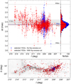 |
Fig. 1. Gaia DR2 ϖ of YSOs with IR-excess in Orion A versus l (top, σϖ as error-bars), and projected YSO distribution displayed on the Herschel map (bottom). Red are YSOs that pass the applied selection criteria as discussed in the first two steps in Sect. 2. The blue sources represent the sources lost when the flux-excess-cut is applied. This highlights that nebulae (near the ONC, see map) cause additional ϖ uncertainties, not reflected in σϖ. The 1D distribution of ϖ for both samples is shown in the histogram on the right. The red and blue middle lines show the median ϖ of the samples. The lower and upper borders (black dashed lines) indicate the applied distance cuts to avoid possible foreground or background contamination when deducing the average distances. The middle gray line shows the distance to the ONC of 414 pc (Menten et al. 2007), while the gray shaded band represents the 2D projected size of the cloud of about 40 pc at 414 pc. |
 |
Fig. 2. Histogram of Gaia DR2 G-band magnitudes. The gray distribution shows all YSOs toward Orion A with measured Gaia DR2 parallaxes. The red and blue distributions show the YSO samples that pass our required selection criteria, while we distinguish sources with (red) and without (blue) flux-excess-cut (see also Fig. 1). |
3. Results
In Fig. 3 we show the average distances, derived from averaged parallaxes of the YSOs per one degree wide bins along Galactic longitude (Δl = 1°, ∼7 pc at 414 pc, over-sampled by a factor of two). We do not weight the average by the parallax errors, given that we have already applied conservative error cuts. The map (Figs. 1 and 3, bottom) shows the YSO distribution projected in Galactic coordinates on a Planck-Herschel-extinction dust column-density map (Lombardi et al. 2014; hereafter, Herschel map)5. The distance variations in Fig. 3 (top) indicate that the Head of the cloud appears to be roughly on the plane of the sky at about 400 pc (for an extent of about 15 pc to 20 pc), while the Tail, starting between l ≈ 210° and 211° and reaching to l ≈ 214.5°, extends from about 400 pc to about 470 pc along the line-of-sight. Thus, the Tail is inclined ∼70° away from the plane of the sky. Consequently, the Tail is about four times as long (∼75 pc) as the Head, leading to a total length of the Orion A filament of about 90 pc.
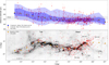 |
Fig. 3. Top: distance estimates (1/ϖ) for YSOs in Orion A versus l and their average distances per Δl. YSOs are shown as red dots with error-bars (σϖ/ϖ2). Over-plotted are the median (blue diamonds) and mean (orange circles) distances per Δl = 1° (blue/green vertical lines on the bottom map correspond to the bin boundaries, factor two over-sampled). The 1σ and 2σ lower and upper percentiles are shown as blue shaded areas. The horizontal gray line represents the Menten et al. (2007) distance to the ONC at 414 pc with a range of ±20 pc (gray shaded area) corresponding to the projected extent in l of the cloud (∼40 pc at 414 pc). Bottom: distribution of the YSOs in Galactic coordinates projected on the Herschel map. The displayed area corresponds to the VISTA observed region (Meingast et al. 2016). The dark shades of the gray scale indicate regions of high dust column-density (or high extinction). The distribution of YSOs follows the high density regions of the cloud, shown by their mean (b) positions per Δl (orange squares). |
The surprising extent of the cloud along the line-of-sight is visualized in Fig. 4, where we project the YSO positions (σϖ as gray scale) in a cartesian plane as seen from the Sun, with XOrion pointing toward Orion A. Over-plotted we show the mean positions per bin (orange dots, as in Fig. 3). The displayed mean positions were transformed into the cartesian coordinate system using the following positions: the mean YSO distances ( ), the mean Galactic latitude positions of the YSOs (
 ), and the Δl bin centers (see also Table 2). Sources with σϖ ≳ 0.085 mas disappear in this visualization, while the scatter of YSO distances is still largest near the ONC. However, since the scatter follows largely the line-of-sight, it is still likely that it reflects parallax measurement uncertainties. This should be kept under review in future Gaia data releases.
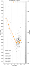 |
Fig. 4. YSO distribution and YSO’s mean positions projected in a cartesian plane. In this coordinate frame the Sun (at X, Y, Z = 0, 0, 0) is connected to the location of Orion A with XOrion pointing toward (l/b)=(211°/−19.5°). Consequently, XOrion is similar to the distance from the Sun, while the YOrion and ZOrion components coincide roughly with the l and b distribution, respectively. The YSOs are shown in gray scale colored by σϖ. The mean positions per Δl are shown as orange filled circles (as in Fig. 3), while the two rightmost points from Fig. 3 are excluded. The gray dashed lines are lines of constant l as viewed from the Sun (2° steps from l = 206° to 216°). For orientation, the numbered boxes show the mean positions of YSOs projected near eight known clusters, as listed in the bottom left legend. In brackets we give the estimated distances (derived from Gaia DR2 parallaxes), which are used to plot the boxes. |
In Fig. 5 we show the orientation of the Orion A cloud projected in Galactic cartesian coordinates, using the mentioned mean YSO positions (Table 2). We exclude the three rightmost positions in Fig. 3 (l ≤ 208°), since they are not projected on top of high dust column-density. Figure 5 highlights the extent of the cloud in galactic 3D space, also showing an idealized representation of the 3D shape of the cloud in gray scale. The shape is deduced by using extinction contours at AK, Herschel
= 0.57 mag (using extinctions from the Herschel map). For the far end of the Tail (l ≥ 213.5°, last three points), we extrapolate the cloud shape manually, since the extinction drops on the upper side of the Tail. We use then the middle b position between the upper and lower edge of the Tail, instead of  . This approach visualizes the opening of the Tail. The sharp turn from Head to Tail is clearly visible in XY and XZ projection. The striking bent of the Head, which consists basically of the integral shaped filament (ISF), calls for a revision of the star-formation history in Orion A.
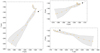 |
Fig. 5. 3D orientation of the Orion A GMC in Galactic cartesian coordinates (X positive toward the Galactic center, Y positive toward the Galactic east, Z positive toward the Galactic north). The orange dots represent the mean positions of YSOs per Δl (see Fig. 3), while only using those on top of high column-density. The gray shaded area shows an idealized 3D cloud shape in each projection at AK, Herschel ≳ 0.57 mag (AV ≳ 5 mag), assuming a symmetric cylindrical shape, meaning that the filament is as deep as it is wide in the sky. For orientation, the black arrows indicate the line-of-sight from the Sun. Each arrow points toward (l, b)=(211.0, −19.5) plotted from d = 380 pc to 390 pc. |
A potential caveat to using the distances of YSOs as proxies to the cloud distance is that Gaia, being an optical telescope, is not sensitive to highly extincted sources. As a consequence, it will miss embedded YSOs and non-embedded YSOs that may be hidden by the cloud. This implies that the derived distances might suffer from a bias toward closer distances (corresponding to the mean separation between YSOs and the cloud), more pronounced at the denser parts. In a first step we tested the average distances by using only sources projected on top of high extinction, by gradually increasing the extinction threshold (from AK, Herschel = 0.1 mag to 1.0 mag with 0.1 mag steps). Secondly, we used only sources projected on low extinction, again using the mentioned extinction thresholds. We find no significant difference in the mean distance distribution, and also the mean distances do not shift systematically to closer distances at high extinctions. With this, we estimate, given the error in the DR2 parallaxes and the source distance distribution, that the averaged distances per bin are approximately reflecting the cloud shape, especially in regions of low extinction. For regions of higher extinction, like the ISF, the distance might be biased toward closer distances, aggravated by the existence of foreground populations (e.g., Alves & Bouy 2012; Bouy et al. 2014) of young stars.
We like to point out that in Fig. 4, the ONC, an especially embedded cluster, appears at about 400–410 pc (close to 414 pc, Menten et al. 2007) while the adjacent regions (including foreground clusters) appear at a distance of about 390 pc. The about 10 pc difference compared to the literature value can be seen as an estimate of remaining systematic uncertainties for the approach we are following. A global systematic parallax offset of 0.08 mas (Stassun & Torres 2018) would produce a shift of about 12 pc toward closer distances at the Head, and of about 16 pc at the Tail. As mentioned in Sect. 2, we do not include a systematic offset in the reported distances, since it is very unclear how it affects sources across Orion A. More importantly for this paper, relative distances are sufficient and the 3D shape of Orion A is largely independent of an offset.
We further test the result by (a) changing the bin size Δl along the cloud from 0.1° to 1.0°, (b) varying the different error cuts, and (c) excluding sources that are not projected near regions of high dust column-density. The overall result stays the same in all cases, with the Tail starting to incline between l ≈ 210° and 211°. Regarding (a), using smaller bins naturally increases noise or reflects the existence of cloud sub-structure, while larger bins have a smoothing effect. It is clear from Fig. 3, that, for example, the region near L1641-South shows some significant distance variations, which hint toward a more complex structure than presented here. In this paper we will not go into detail about specific sub-structures or sub-clusters in Orion A, since we are only interested in the overall shape and line-of-sight extent. A more detailed analysis of this important cloud is called for, using future Gaia data releases, which will provide improved accuracy.
In Table 3 we provide average distances of large-scale sub-regions in Orion A. We find that YSOs at the Head of the cloud, including the ISF region, the ONC, NGC1977, NGC1981, NGC1980, and L1641-North, lie on average at about 395 pc. YSOs at the Tail are on average at about 430 pc, including L1641-Center and South, and L1647-North and South. Separating the very southern part (L1647-South), we get a maximum distance to the end of the Tail of about 470 pc, while the most distant stars have distances of about 550 pc. We find that the two clusters L1647-North and South are more distant (420 pc–470 pc) than estimated with X-ray luminosities (250 pc–280 pc, Pillitteri et al. 2016). To make this a fair comparison, we investigate the DR2 parallaxes of XMM-Newton X-ray sources6 in this region, which show a similar average distance as the IR-excess YSOs, supporting the farther distance estimated toward these clusters. The resulting tension between the X-ray luminosities and the Gaia results need further investigation.
The main result in this paper confirms previous work who pointed out a distance gradient in Orion A, as already discussed in Sect. 1. The ∼70 pc distance difference from Head to Tail is in agreement with Schlafly et al. (2014), while the individual values along the cloud show variations between the samples (see Tables 1, 2, and 3). Kounkel et al. (2017) discuss the 3D orientation of Orion A using VLBI measurements in the ONC and L1641-South. The ∼40 pc distance difference between these regions is again in agreement with our findings. Kounkel et al. (2018), who also use Gaia DR2 parallaxes of young stars, find a smaller distance difference from Head to Tail as compared to our result (about 55 pc from ONC to L1647). The discrepancy is due to the different samples used. In this paper we use only the highest-quality data for the youngest YSOs (ages ≲3 Myr), as these are likely to be the closest sources to the cloud, while Kounkel et al. (2018) aims at maximizing the identification of young stars in the entire Orion star-forming region, and includes sources as old as 12 Myr. For completeness, we compare our sample to the Kounkel et al. (2018) sample (K18) and we find that only about 20% of their sources are in common with our sample (or about 68% of our sample are in common with K18). The rest of the K18 sources (80%) are likely older and less connected to the Orion A cloud, hence, not good tracers of the cloud’s shape. The sources which are only in our sample (about 1/3 of our sample) are further responsible for the different results. We find that some of these sources are more distant, especially near the Tail.
While these three papers (Schlafly et al. 2014; Kounkel et al. 2017, 2018) point to a gradient in the distance from the Head to the Tail of the cloud, our paper not only confirms this gradient, but (1) establishes that the Head of the cloud is bent in regards to the Tail, (2) the Head is essentially on the plane of the sky while the tail appears to be highly inclined, not far from the line-of-sight, and (3) that the cloud has overall a cometary-like shape oriented toward the Galactic plane, although containing sub-structure not resolved in our reconstruction.
Furthermore, our results are in agreement with Kuhn et al. (2018) and Stutz et al. (2018). Kuhn et al. (2018) investigate the kinematics of the ONC using Chandra observed cluster members in combination with Gaia DR2. They report a distance of about 403 pc to the ONC (Table 1), similar to the estimated 407 pc that we find, when looking solely at YSOs near the ONC (Fig. 4). They point out that the ONC seems to be recessed relative to the immediate surroundings (at ∼395 pc), which we also observe by using IR-excess YSOs (see Figs. 1 or 3 and Fig. 21 in Kuhn et al. 2018). A similar situation is presented in Stutz et al. (2018), where they also find that the ONC region is about 10 pc recessed with respect to its surroundings.
Mean positions per Galactic longitude bin (Δl).
Averaged parallaxes and derived distances to different large-scale sub-regions in Orion A.
4. Discussion
The 3D shape of Orion A, now accessible via the Gaia measurements, informs and enlightens our knowledge on this fundamental star-formation benchmark. The main result from this work is that Orion A is longer than previously assumed and has a cometary shape pointing toward the Galactic plane. Also of note, the Head of the cloud appears to be bent in comparison with the Tail (Fig. 5). Why would this be the case? One important hint is that the star-formation rate in the Head of the cloud is about an order of magnitude higher than in the Tail (Großscheld et al., in prep.). Taking this into consideration, one can think of at least two scenarios to explain the enhanced star-formation rate and the shape of the Head: (1) cloud-cloud collision and (2) feedback from young stars and supernovae. Recently, Fukui et al. (2018) interpreted the gas velocities in this region as evidence that two clouds collided about 0.1 Myr ago, and are likely responsible for the formation of the massive stars. While we cannot rule out this scenario with the data presented here, we point out that there is evidence for a young population of foreground massive stars (e.g., in NGC 1980, NGC 1981, Bally 2008; Alves & Bouy 2012; Bouy et al. 2014; cf. Fang et al. 2017), that could provide the feedback necessary to bend the Head of the cloud. An investigation on the second scenario is needed and beyond the scope of this work, but it seems plausible that an external event to the Orion A cloud could have taken place in the last million years.
The 3D shape of the cloud clarifies some previous results. For example, Meingast et al. (2018) found evidence for different dust properties in Orion A, when comparing the regions in the Head and the Tail of the cloud. They argued, correctly, that the dust in L1641 might not “see” the radiation from the massive stars toward the Head of the cloud, and their properties are then not affected by it. Our result validates this view: the dust grains in L1641 lie substantially in the back of the ONC, which contains the most massive stars in the region, and are hence shielded, or too far from the sources of UV radiation.
The deduced length of the Orion A filament of 90 pc makes it similar to the Nessie Classic filament (∼80 pc, Jackson et al. 2010), which is often regarded as a prototypical large-scale filament, or a “bone” of the Milky Way (Goodman et al. 2014). Zucker et al. (2017) undertook an analysis of the physical properties and kinematics of a sample of 45 large-scale filaments in the literature. They found that these filaments can be distinguished in three broad categories, depending on their aspect ratio and high column-density fraction. Orion A has an average aspect ratio of about 30:1 when taking the length of 90 pc and its average width (FWHM ∼ 3 pc), and a high-column-density fraction of about 45%. For the latter we use an AK threshold of 0.5 mag, comparable to 1 × 1022 cm−2 in Zucker et al. (2017). This puts Orion A squarely into their category (c), which describes highly elongated, high-column-density filaments, or so called “bones” of the Milk Way. The position-angle between Orion A and the plane is in agreement with the average position-angles of the bones in their sample, but Orion A differs significantly from the known bones regarding its distance from the mid-plane of the Milky Way (∼145 pc), which is an order of magnitude larger than the median distance between bones and the Galactic plane. This discrepancy calls for a large-scale process to have pushed the cloud this far from the plane. Franco (1986) proposed a scenario for the origin of the Orion complex as the consequence of an impact of a high-velocity cloud with the plane of the Galaxy (from above) that could account for the abnormal distance of Orion below the plane. Nevertheless, the cloud’s cometary shape with a star-bursting Head closer to the plane, as shown in this work, seems to be at odds with this scenario.
Finally, we point out that the unexpected length of Orion A along the line-of-sight affects the observables toward the cloud (masses, luminosities, binary separations) that will need revision. For example, the current cloud and YSO masses toward the Tail can be underestimated by about 30%–40% under the common assumption of a single constant distance to Orion A, while binary separations can be underestimated by about 10%–20%.
5. Summary
We have used the recent Gaia DR2 to investigate the 3D shape of the Orion A GMC. Orion A is not the straight filamentary cloud that we see in (2D) projection, but instead a cometary-like cloud, oriented toward the Galactic plane, with two distinct components: a denser and enhanced star-forming (bent) Head, and a lower density and star-formation quieter ∼75 pc long Tail. The two components seem to overlap between l ≈ 210° to 211°. We find that the Head of the Orion A cloud appears to be roughly on the plane of the sky (at ∼400 pc), while the Tail, surprisingly, appears to be highly inclined, not far from the line-of-sight (∼70°), reaching at least ∼470 pc. The true extent of Orion A is then not the projected ∼40 pc but ∼90 pc, making it by far the largest molecular cloud in the local neighborhood. Its aspect ratio (∼30:1) and high-column-density fraction (∼45%) make it similar to large-scale Milky Way filaments (bones), despite its distance to the galactic mid-plane being an order of magnitude larger than typically found for these structures. Gaia is opening an important new window in the study of the ISM, in particular the star-forming ISM, bringing the critical third spatial dimension that will allow not only cloud structure studies similar to the ones presented here, but an unique view on the dynamics between dense gas and YSOs.
For simplicity we classify the Orion A cloud roughly into Head and Tail; the Tail represents the less star-forming part.
Shortcuts for Gaia parameters:
ϖ: parallax [mas]
σϖ: parallax_error [mas]
G: phot_g_mean_mag [mag]
σG : 1.0857/phot_g_mean_flux_over_error [mag]
ϵi: astrometric_excess_noise [mas]
sig_ϵi: astrometric_excess_noise_sig (significance).
Using the ratio of the fluxes (IBP − IRP)/IG:
phot_bp_rp_excess_factor.
Bright sources with G < 6 mag have generally inferior astrometric quality. Faint sources with G > 18 mag are problematic in dense regions.
We use a factor 3050 to linearly convert Herschel optical depth to extinction, as derived by Meingast et al. (2018).
Acknowledgments
We thank the anonymous referee whose comments helped to improve the manuscript. J. Großschedl acknowledges funding by the Austrian Science Fund (FWF) under project number P 26718-N27. This work is based on observations made with ESO Telescopes at the La Silla Paranal Observatory under program ID 090.C-0797(A). This work is part of the research program VENI with project number 639.041.644, which is (partly) financed by the Netherlands Organisation for Scientific Research (NWO). A. Hacar thanks the Spanish MINECO for support under grant AYA2016-79006-P. This work has made use of data from the European Space Agency (ESA) mission Gaia (https://www.cosmos.esa.int/gaia), processed by the Gaia Data Processing and Analysis Consortium (DPAC, https://www.cosmos.esa.int/web/gaia/dpac/consortium). Funding for the DPAC has been provided by national institutions, in particular the institutions participating in the Gaia Multilateral Agreement. This research has made use of the VizieR catalog access tool, CDS, Strasbourg, France. This research has made use of Python, https://www.python.org, of Astropy, a community-developed core Python package for Astronomy (Astropy Collaboration 2013), NumPy (Van Der Walt et al. 2011), and Matplotlib (Hunter 2007). This research made use of TOPCAT, an interactive graphical viewer and editor for tabular data (Taylor 2005). This work has made use of “Aladin sky atlas” developed at CDS, Strasbourg Observatory, France (Bonnarel et al. 2000; Boch & Fernique 2014).
References
- Alves, J., & Bouy, H. 2012, A&A, 547, A97 [NASA ADS] [CrossRef] [EDP Sciences] [Google Scholar]
- Arenou, F., Luri, X., Babusiaux, C., et al. 2018, A&A, 616, A17 [Google Scholar]
- Astropy Collaboration, Robitaille, T. P., Tollerud, E. J., et al. 2013, A&A, 558, A33 [NASA ADS] [CrossRef] [EDP Sciences] [Google Scholar]
- Bailer-Jones, C. A. L., Rybizki, J., Fouesneau, M., Mantelet, G., & Andrae, R. 2018, AJ, 158, 58 [NASA ADS] [CrossRef] [Google Scholar]
- Bally, J. 2008, Handbook of Star Forming Regions, 64, 459 [NASA ADS] [Google Scholar]
- Boch, T., & Fernique, P. 2014, in Astronomical Data Analysis Software and Systems XXIII, eds. N. Manset, & P. Forshay, ASP Conf. Ser., 485, 277 [NASA ADS] [Google Scholar]
- Bonnarel, F., Fernique, P., Bienaymé, O., et al. 2000, A&AS, 143, 33 [NASA ADS] [CrossRef] [EDP Sciences] [Google Scholar]
- Bouy, H., Alves, J., Bertin, E., Sarro, L. M., & Barrado, D. 2014, A&A, 564, A29 [NASA ADS] [CrossRef] [EDP Sciences] [Google Scholar]
- Evans, D. W., Riello, M., De Angeli, F., et al. 2018, A&A, 616, A4 [NASA ADS] [CrossRef] [EDP Sciences] [Google Scholar]
- Fang, M., Kim, J. S., Pascucci, I., et al. 2017, AJ, 153, 188 [Google Scholar]
- Franco, J. 1986, Rev. Mex. Astron. Astrofis., 12, 287 [NASA ADS] [Google Scholar]
- Fukui, Y., Torii, K., Hattori, Y., et al. 2018, ApJ, 859, 166 [NASA ADS] [CrossRef] [Google Scholar]
- Furlan, E., Fischer, W. J., Ali, B., et al. 2016, ApJS, 224, 5 [NASA ADS] [CrossRef] [Google Scholar]
- Gaia Collaboration (Babusiaux, C., et al.) 2018a, A&A, 616, A10 [NASA ADS] [CrossRef] [EDP Sciences] [Google Scholar]
- Gaia Collaboration (Brown, A. G. A., et al.) 2018b, A&A , 616, A1 [NASA ADS] [CrossRef] [EDP Sciences] [Google Scholar]
- Genzel, R., Reid, M. J., Moran, J. M., & Downes, D. 1981, ApJ, 244, 884 [NASA ADS] [CrossRef] [Google Scholar]
- Goodman, A. A., Alves, J., Beaumont, C. N., et al. 2014, ApJ, 797, 53 [NASA ADS] [CrossRef] [Google Scholar]
- Green, G. M., Schlafly, E. F., Finkbeiner, D. P., et al. 2014, ApJ, 783, 114 [NASA ADS] [CrossRef] [Google Scholar]
- Großschedl, J. E., Alves, J., Teixeira, P. S., et al. 2018, A&A, accepted [arXiv:1810.00878] [Google Scholar]
- Hacar, A., Alves, J., Forbrich, J., et al. 2016, A&A, 589, A80 [NASA ADS] [CrossRef] [EDP Sciences] [Google Scholar]
- Hirota, T., Bushimata, T., Choi, Y. K., et al. 2007, PASJ, 59, 897 [NASA ADS] [CrossRef] [Google Scholar]
- Hunter, J. D. 2007, Comput. Sci. Eng., 9, 90 [Google Scholar]
- Jackson, J. M., Finn, S. C., Chambers, E. T., Rathborne, J. M., & Simon, R. 2010, ApJ, 719, L185 [NASA ADS] [CrossRef] [Google Scholar]
- Kim, M. K., Hirota, T., Honma, M., et al. 2008, PASJ, 60, 991 [NASA ADS] [CrossRef] [Google Scholar]
- Kounkel, M., Hartmann, L., Loinard, L., et al. 2017, ApJ, 834, 142 [NASA ADS] [CrossRef] [Google Scholar]
- Kounkel, M., Covey, K., Suarez, G., et al. 2018, AJ, 156, 84 [NASA ADS] [CrossRef] [Google Scholar]
- Kuhn, M. A., Hillenbrand, L. A., Sills, A., Feigelson, E. D. & Getman, K. V. 2018, Astrophys. Galaxies, submitted, [Google Scholar]
- Lewis, J. A., & Lada, C. J. 2016, ApJ, 825, 91 [NASA ADS] [CrossRef] [Google Scholar]
- Lindegren, L., Hernandez, J., Bombrun, A., et al. 2018, A&A, 616, A2 [NASA ADS] [CrossRef] [EDP Sciences] [Google Scholar]
- Lombardi, M., Alves, J., & Lada, C. J. 2011, A&A, 535, A16 [NASA ADS] [CrossRef] [EDP Sciences] [Google Scholar]
- Lombardi, M., Bouy, H., Alves, J., & Lada, C. J. 2014, A&A, 568, C1 [Google Scholar]
- Megeath, S. T., Gutermuth, R., Muzerolle, J., et al. 2012, AJ, 144, 192 [NASA ADS] [CrossRef] [Google Scholar]
- Megeath, S. T., Gutermuth, R., Muzerolle, J., et al. 2016, AJ, 151, 5 [NASA ADS] [CrossRef] [Google Scholar]
- Meingast, S., Alves, J., Mardones, D., et al. 2016, A&A, 587, A153 [NASA ADS] [CrossRef] [EDP Sciences] [Google Scholar]
- Meingast, S., Alves, J., & Lombardi, M. 2018, A&A, 614, A65 [NASA ADS] [CrossRef] [EDP Sciences] [Google Scholar]
- Menten, K. M., Reid, M. J., Forbrich, J., & Brunthaler, A. 2007, A&A, 474, 515 [NASA ADS] [CrossRef] [EDP Sciences] [Google Scholar]
- Muench, A., Getman, K., Hillenbrand, L. & Preibisch, T. 2008, in Star Formation in the Orion Nebula I: Stellar Content, ed. B. Reipurth, 483 [Google Scholar]
- Pillitteri, I., Wolk, S. J., & Megeath, S. T. 2016, ApJ, 820, L28 [NASA ADS] [CrossRef] [Google Scholar]
- Sandstrom, K. M., Peek, J. E. G., Bower, G. C., Bolatto, A. D., & Plambeck, R. L. 2007, ApJ, 667, 1161 [NASA ADS] [CrossRef] [Google Scholar]
- Schlafly, E. F., Green, G., Finkbeiner, D. P., et al. 2014, ApJ, 786, 29 [NASA ADS] [CrossRef] [Google Scholar]
- Stassun, K. G., & Torres, G. 2018, Solar Stellar Astrophys., submitted. [Google Scholar]
- Stutz, A. M., Gonzalez-Lobos, V. I., & Gould, A. 2018, MNRAS, submitted [arXiv:1807.11496] [Google Scholar]
- Taylor, M. B. 2005, in Astronomical Data Analysis Software and Systems XIV, eds. P. Shopbell, M. Britton, & R. Ebert, ASP Conf. Ser., 347, 29 [Google Scholar]
- Tobin, J. J., Hartmann, L., Furesz, G., Mateo, M., & Megeath, S. T. 2009, ApJ, 697, 1103 [NASA ADS] [CrossRef] [Google Scholar]
- Van Der Walt, S., Colbert, S. C., & Gaël, V. 2011, Comput. Sci. Eng., 13, 22 [CrossRef] [Google Scholar]
- Zucker, C., Battersby, C., & Goodman, A. 2017, ApJ, submitted. [Google Scholar]
Appendix A: Additional figure
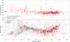 |
Fig. A1. YSO distribution and distance estimates toward Orion A, similar to Figs. 1 and 3. Additionally we show the positions of measured distances from the Literature. The gray band shows the distance of 414 ± 7 pc from Menten et al. (2007). Blue boxes are the reported distances from Kounkel et al. (2017; VLBA parallaxes). Green diamonds show distances to certain positions as given in Schlafly et al. (2014; optical reddening). The reported distances from previous works are largely in agreement with Gaia DR2 distances of YSOs, within the errors and the scatter. See also Table 1. |
Appendix B: YSO table
Catalog of the 682 YSOs, used to infer on the cloud’s shape.
All Tables
Averaged parallaxes and derived distances to different large-scale sub-regions in Orion A.
All Figures
|
Fig. 1. Gaia DR2 ϖ of YSOs with IR-excess in Orion A versus l (top, σϖ as error-bars), and projected YSO distribution displayed on the Herschel map (bottom). Red are YSOs that pass the applied selection criteria as discussed in the first two steps in Sect. 2. The blue sources represent the sources lost when the flux-excess-cut is applied. This highlights that nebulae (near the ONC, see map) cause additional ϖ uncertainties, not reflected in σϖ. The 1D distribution of ϖ for both samples is shown in the histogram on the right. The red and blue middle lines show the median ϖ of the samples. The lower and upper borders (black dashed lines) indicate the applied distance cuts to avoid possible foreground or background contamination when deducing the average distances. The middle gray line shows the distance to the ONC of 414 pc (Menten et al. 2007), while the gray shaded band represents the 2D projected size of the cloud of about 40 pc at 414 pc. |
| In the text | |
|
Fig. 2. Histogram of Gaia DR2 G-band magnitudes. The gray distribution shows all YSOs toward Orion A with measured Gaia DR2 parallaxes. The red and blue distributions show the YSO samples that pass our required selection criteria, while we distinguish sources with (red) and without (blue) flux-excess-cut (see also Fig. 1). |
| In the text | |
|
Fig. 3. Top: distance estimates (1/ϖ) for YSOs in Orion A versus l and their average distances per Δl. YSOs are shown as red dots with error-bars (σϖ/ϖ2). Over-plotted are the median (blue diamonds) and mean (orange circles) distances per Δl = 1° (blue/green vertical lines on the bottom map correspond to the bin boundaries, factor two over-sampled). The 1σ and 2σ lower and upper percentiles are shown as blue shaded areas. The horizontal gray line represents the Menten et al. (2007) distance to the ONC at 414 pc with a range of ±20 pc (gray shaded area) corresponding to the projected extent in l of the cloud (∼40 pc at 414 pc). Bottom: distribution of the YSOs in Galactic coordinates projected on the Herschel map. The displayed area corresponds to the VISTA observed region (Meingast et al. 2016). The dark shades of the gray scale indicate regions of high dust column-density (or high extinction). The distribution of YSOs follows the high density regions of the cloud, shown by their mean (b) positions per Δl (orange squares). |
| In the text | |
|
Fig. 4. YSO distribution and YSO’s mean positions projected in a cartesian plane. In this coordinate frame the Sun (at X, Y, Z = 0, 0, 0) is connected to the location of Orion A with XOrion pointing toward (l/b)=(211°/−19.5°). Consequently, XOrion is similar to the distance from the Sun, while the YOrion and ZOrion components coincide roughly with the l and b distribution, respectively. The YSOs are shown in gray scale colored by σϖ. The mean positions per Δl are shown as orange filled circles (as in Fig. 3), while the two rightmost points from Fig. 3 are excluded. The gray dashed lines are lines of constant l as viewed from the Sun (2° steps from l = 206° to 216°). For orientation, the numbered boxes show the mean positions of YSOs projected near eight known clusters, as listed in the bottom left legend. In brackets we give the estimated distances (derived from Gaia DR2 parallaxes), which are used to plot the boxes. |
| In the text | |
|
Fig. 5. 3D orientation of the Orion A GMC in Galactic cartesian coordinates (X positive toward the Galactic center, Y positive toward the Galactic east, Z positive toward the Galactic north). The orange dots represent the mean positions of YSOs per Δl (see Fig. 3), while only using those on top of high column-density. The gray shaded area shows an idealized 3D cloud shape in each projection at AK, Herschel ≳ 0.57 mag (AV ≳ 5 mag), assuming a symmetric cylindrical shape, meaning that the filament is as deep as it is wide in the sky. For orientation, the black arrows indicate the line-of-sight from the Sun. Each arrow points toward (l, b)=(211.0, −19.5) plotted from d = 380 pc to 390 pc. |
| In the text | |
|
Fig. A1. YSO distribution and distance estimates toward Orion A, similar to Figs. 1 and 3. Additionally we show the positions of measured distances from the Literature. The gray band shows the distance of 414 ± 7 pc from Menten et al. (2007). Blue boxes are the reported distances from Kounkel et al. (2017; VLBA parallaxes). Green diamonds show distances to certain positions as given in Schlafly et al. (2014; optical reddening). The reported distances from previous works are largely in agreement with Gaia DR2 distances of YSOs, within the errors and the scatter. See also Table 1. |
| In the text | |
Current usage metrics show cumulative count of Article Views (full-text article views including HTML views, PDF and ePub downloads, according to the available data) and Abstracts Views on Vision4Press platform.
Data correspond to usage on the plateform after 2015. The current usage metrics is available 48-96 hours after online publication and is updated daily on week days.
Initial download of the metrics may take a while.