| Issue |
A&A
Volume 619, November 2018
|
|
|---|---|---|
| Article Number | A159 | |
| Number of page(s) | 11 | |
| Section | Extragalactic astronomy | |
| DOI | https://doi.org/10.1051/0004-6361/201833618 | |
| Published online | 20 November 2018 | |
Detection of persistent VHE gamma-ray emission from PKS 1510–089 by the MAGIC telescopes during low states between 2012 and 2017
1
Inst. de Astrofísica de Canarias, Universidad de La Laguna, Dpto. Astrofísica, 38206 La Laguna, Tenerife, Spain
2
Università di Udine, 33100 Udine, Italy
3
INFN Trieste, 34149 Trieste, Italy
4
National Institute for Astrophysics (INAF), 00136 Rome, Italy
5
ETH Zurich, 8093 Zurich, Switzerland
6
Università di Padova, 35131 Padova, Italy
7
INFN Padova, 35131 Padova, Italy
8
Technische Universität Dortmund, 44221 Dortmund, Germany
9
Croatian MAGIC Consortium: University of Rijeka, 51000 Rijeka; University of Split – FESB, 21000 Split; University of Zagreb – FER, 10000 Zagreb; University of Osijek, 31000 Osijek and Rudjer Boskovic Institute, 10000 Zagreb, Croatia
10
Saha Institute of Nuclear Physics, HBNI, 1/AF Bidhannagar, Salt Lake, Sector-1, Kolkata 700064, India
11
Max-Planck-Institut für Physik, 80805 München, Germany
12
Centro Brasileiro de Pesquisas Físicas (CBPF), 22290-180 URCA, Rio de Janeiro, RJ, Brasil
13
Unidad de Partículas y Cosmología (UPARCOS), Universidad Complutense, 28040 Madrid, Spain
14
University of ᴌódź, Department of Astrophysics, 90236 ᴌódź, Poland
15
Deutsches Elektronen-Synchrotron (DESY), 15738 Zeuthen, Germany
16
Institut de Física d’Altes Energies (IFAE), The Barcelona Institute of Science and Technology (BIST), 08193 Bellaterra, Barcelona, Spain
17
Università di Siena, 53100 Siena, Italy
18
INFN Pisa, 56127 Pisa, Italy
19
Università di Pisa, 56126 Pisa, Italy
20
Universität Würzburg, 97074
Würzburg, Germany
21
Finnish MAGIC Consortium: Tuorla Observatory (Department of Physics and Astronomy) and Finnish Centre of Astronomy with ESO (FINCA), University of Turku, 20014 Turku, Finland; Astronomy Division, University of Oulu, 90014 Oulu, Finland
22
Departament de Física, and CERES-IEEC, Universitat Autónoma de Barcelona, 08193 Bellaterra, Spain
23
Universitat de Barcelona, ICCUB, IEEC-UB, 08028 Barcelona, Spain
24
Japanese MAGIC Consortium: ICRR, The University of Tokyo, 277-8582 Chiba, Japan; Department of Physics, Kyoto University, 606-8502 Kyoto, Japan; Tokai University, 259-1292 Kanagawa, Japan; RIKEN, 351-0198 Saitama, Japan
25
Inst. for Nucl. Research and Nucl. Energy, Bulgarian Academy of Sciences, 1784 Sofia, Bulgaria
26
Humboldt University of Berlin, Institut für Physik, 12489 Berlin, Germany
27
Dipartimento di Fisica, Università di Trieste, 34127 Trieste, Italy
28
Port d’Informació Científica (PIC), 08193 Bellaterra, Barcelona, Spain
29
INAF-Trieste and Dept. of Physics & Astronomy, University of Bologna, Italy
30
INAF, Osservatorio Astrofisico di Torino, Via Osservatorio 20, 10025 Pino Torinese, Italy
31
Università dell’Insubria, Dipartimento di Scienza ed Alta Tecnologia, Via Valleggio 11, 22100 Como, Italy
32
INAF-Istituto Nazionale di Astrofisica, Osservatorio Astronomico di Brera, Via Bianchi 46, 23807 Merate, LC, Italy
33
Owens Valley Radio Observatory, California Institute of Technology, Pasadena, CA 91125, USA
34
Tuorla Observatory, University of Turku, Väisäläntie 20, 21500 Piikkiö, Finland
35
Departamento de Astronomía, Universidad de Chile, Camino El Observatorio 1515, Las Condes, Santiago, Chile
36
Aalto University Metsähovi Radio Observatory, Metsähovintie 114, 02540 Kylmälä, Finland
37
Aalto University Department of Electronics and Nanoengineering, PO Box 15500, 00076 Aalto, Finland
38
Tartu Observatory, Observatooriumi 1, 61602 Tõravere, Estonia
39
Instituto de Radio Astronomía Millimétrica, Avenida Divina Pastora, 7, Local 20, 18012 Granada, Spain
40
Instituto de Astrofísica de Andalucía (CSIC), Apartado 3004, 18080 Granada, Spain
41
Max-Planck-Institut für Radioastronomie, Auf dem Hügel, 69, 53121
Bonn, Germany
Received:
12
June
2018
Accepted:
31
August
2018
Abstract
Context. PKS 1510–089 is a flat spectrum radio quasar strongly variable in the optical and GeV range. To date, very high-energy (VHE, > 100 GeV) emission has been observed from this source either during long high states of optical and GeV activity or during short flares.
Aims. We search for low-state VHE gamma-ray emission from PKS 1510–089. We characterize and model the source in a broadband context, which would provide a baseline over which high states and flares could be better understood.
Methods. PKS 1510–089 has been monitored by the MAGIC telescopes since 2012. We use daily binned Fermi-LAT flux measurements of PKS 1510–089 to characterize the GeV emission and select the observation periods of MAGIC during low state of activity. For the selected times we compute the average radio, IR, optical, UV, X-ray, and gamma-ray emission to construct a low-state spectral energy distribution of the source. The broadband emission is modeled within an external Compton scenario with a stationary emission region through which plasma and magnetic fields are flowing. We also perform the emission-model-independent calculations of the maximum absorption in the broad line region (BLR) using two different models.
Results. The MAGIC telescopes collected 75 hr of data during times when the Fermi-LAT flux measured above 1 GeV was below 3 × 10⁻⁸ cm−2 s−1, which is the threshold adopted for the definition of a low gamma-ray activity state. The data show a strongly significant (9.5σ) VHE gamma-ray emission at the level of (4.27 ± 0.61stat) × 10−12 cm−2 s−1 above 150 GeV, a factor of 80 lower than the highest flare observed so far from this object. Despite the lower flux, the spectral shape is consistent with earlier detections in the VHE band. The broadband emission is compatible with the external Compton scenario assuming a large emission region located beyond the BLR. For the first time the gamma-ray data allow us to place a limit on the location of the emission region during a low gamma-ray state of a FSRQ. For the used model of the BLR, the 95% confidence level on the location of the emission region allows us to place it at a distance > 74% of the outer radius of the BLR.
Key words: galaxies: active / galaxies: jets / gamma rays: galaxies / quasars: individual: PKS 1510–089
Corresponding authors: J. Sitarek (e-mail: This email address is being protected from spambots. You need JavaScript enabled to view it. ), C. Nigro (e-mail: This email address is being protected from spambots. You need JavaScript enabled to view it. ), J. Becerra Gonzalez (e-mail: This email address is being protected from spambots. You need JavaScript enabled to view it. ).
© ESO 2018
1. Introduction
PKS 1510–089 is a bright flat spectrum radio quasar (FSRQ) located at a redshift of z = 0.36 (Tanner et al. 1996). It was the second FSRQ to be detected in the very high-energy (VHE, > 100 GeV) range (H.E.S.S. Collaboration 2013). The source is monitored by various instruments spanning the full range from radio up to VHE gamma rays (see, e.g., Marscher et al. 2010; Aleksić et al. 2014; Ahnen et al. 2017a). Similarly to other FSRQs, the GeV gamma-ray emission of PKS 1510–089 is strongly variable (Abdo et al. 2010; Brown 2013; Saito et al. 2013; Prince et al. 2017). Multiple optical flares have been observed from PKS 1510–089 (Liller & Liller 1975; Zacharias et al. 2017a)1.
Significant VHE gamma-ray emission from PKS 1510–089 has been observed on a few occasions: during enhanced optical and GeV states in 2009 (H.E.S.S. Collaboration 2013) and 2012 (Aleksić et al. 2014) and during short flares in 2015 (Ahnen et al. 2017a; Zacharias et al. 2017a) and 2016 (Zacharias et al. 2017b). Interestingly, no variability in VHE gamma rays has been observed during (or between) the high optical/GeV states in 2009 and 2012 (H.E.S.S. Collaboration 2013; Aleksić et al. 2014).
The GeV state of PKS 1510–089 can be studied using the Fermi-LAT all-sky monitoring data. MAGIC is a system of two Imaging Atmospheric Cherenkov Telescopes designed for observations of gamma rays with energies from a few tens of GeV up to a few tens of TeV (Aleksić et al. 2016a). Since the detection of VHE gamma-ray emission from PKS 1510–089 in 2012, a monitoring program is being performed with the MAGIC telescopes. The aimed cadence of monitoring is two to six pointings per month, with individual exposures of 1–3 hr. The source is visible by MAGIC five months of the year. We use the Fermi-LAT data to select periods of low gamma-ray emission of PKS 1510–089. Then we select a subsample of the MAGIC telescope data taken between 2012 and 2017, and contemporaneous multiwavelength data from a number of other instruments in order to study the quiescent VHE gamma-ray state of the source. Such low emission can then be used as a baseline for modeling the flaring states.
In Sect. 2 we briefly introduce the instruments that provided multiwavelength data, describe the data reduction procedures and explain the principle of low-state data selection. In Sect. 3 we present the results of the observations, and the broadband emission modeling is illustrated in Sect. 4. In Sect. 5 we use the gamma-ray spectrum of PKS 1510–089 to evaluate the absorption of sub-TeV photons in the radiation field of the BLR. The most important findings are summarized in Sect. 6.
2. Data
The continuous monitoring of PKS 1510–089 in the GeV band provided by Fermi-LAT allows us to identify the low emission states of the source. Multiwavelength light curves from the radio band up to the GeV band are shown in Fig. 1.
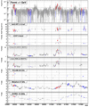 |
Fig. 1. Multiwavelength light curve of PKS 1510–089 between 2012 and 2017. From top to bottom panels: Fermi-LAT flux above 1 GeV; Swift-XRT flux 2–10 keV; U band flux from UVOT; KVA, SMARTS and MAPCAT optical flux in R-band; IR flux from REM and SMARTS in J band; radio 229 GHz flux measured by POLAMI; radio 37 GHz flux measured by Metsähovi; 15 GHz flux measured by OVRO. The red points show the observations within 12 h (or 3 days for the radio measurements) when MAGIC data have been taken during the time that Fermi-LAT flux is above 3 × 10⁻⁸ cm−2 s−1, while the blue points are observations in time bins with Fermi-LAT flux below this flux value (i.e., the low-state sample). IR, optical and UV data have been dereddened using Schlafly & Finkbeiner (2011). |
2.1. Fermi-LAT
Fermi-LAT monitors the high-energy gamma-ray sky in the energy range from 20 MeV to beyond 300 GeV (Atwood et al. 2009). For this work, we analyzed the Pass 8 SOURCE class events within a region of interest (ROI) of 10° radius centered at the position of PKS 1510–089 in the energy range from 100 MeV to 300 GeV. A zenith angle cut of < 90° was applied to reduce the contamination from the Earth’s limb. The analysis was performed with the ScienceTools software package version v11r7p0 using the P8R2_SOURCE_V62 instrument response function and the gll_iem_v06 and iso_P8R2_SOURCE_V6_v06 models3 for the Galactic and isotropic diffuse emission (Acero et al. 2016), respectively.
A first unbinned likelihood fit was performed for the events collected within five months, from 01 February to 30 June 2013 (MJD 56324–56474), using gtlike and including in the model file all 3FGL catalog sources (Acero et al. 2015) of 20° from PKS 1510–089. We repeat the same five-month analysis using the preliminary eight-year Source List4 instead of the 3FGL catalog to search for bright sources within 20° of PKS 1510–089. No new strong sources were found. The model generated from the 3FGL catalog was used for the subsequent analysis. As we are interested in short timescale (daily) fluxes of PKS 1510–089, the purpose of this first fit is to identify weak nearby sources that can be removed from the source model, thus simplifying it. Hence, the sources with a test statistic (TS; Mattox et al. 1996) below 5 were removed from the model file. Next, the optimized output model file was used to produce the PKS 1510–089 light curve with one-day time bins above 1 GeV in the full time period from 5 December 2011 to 7 August 2017 (MJD 55900–57972). The same optimized output model is later also used for the spectral analysis. In the light curve calculations the spectra of PKS 1510–089 were modeled as a power law leaving both the flux normalization and the spectral index as free parameters. The normalization of the Galactic and isotropic diffuse emission models was left to vary freely during the calculation of both the light curves and the spectrum. In addition, the spectra of all sources except PKS 1510–089 and the highly variable source 3FGL 1532.7-1319 (located 6.45° from PKS 1510–089, and having a variability index of 1924.7 from the 3FGL catalog) were fixed to the catalog values.
In order to estimate when the flux can be considered to be in a low state, we first calculate a light curve in relatively wide bins of 30 days in the full time period. This allows us to estimate the flux with relative uncertainty ≲20% for all the points and hence disentangle intrinsic variability from the fluctuations of the measured flux induced by statistical uncertainties. In Fig. 2 we present the distribution of the flux above 1 GeV, which shows that during the low state the flux is in the range (1 − 3)×10−8 cm−2 s−1 in contrast to the value of > 3 × 10⁻⁸ cm−2 s−1 during active (flaring) periods. Hence, we select the days of low state if
 (1)
(1)
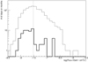 |
Fig. 2. Distribution of flux above 1 GeV measured with Fermi-LAT in 30-day (thick line) or 1-day (thin line) bins. The vertical dashed line shows the value of the cut separating the low state. |
The cut separates the low-flux peak of the daily fluxes distribution from the power-law extension of the high-flux days (see Fig. 2). The effect that choosing a different energy threshold would have on the data selection is discussed in Appendix A. We note, however, that due to the low state and short exposure times the flux measurements during single nights are quite uncertain. The typical uncertainty of the flux in those time bins is ∼1.5 × 10⁻⁸ cm−2 s−1. We also include in the low-state sample nights for which the Fermi-LAT flux did not reach TS of 4. The average 95% confidence level (C.L.) flux upper limit on those nights is also ∼3 × 10⁻⁸ cm−2 s−1.
For the low-state spectrum we combine individual one-day integration windows selected with flux fulfilling Eq. (1). The spectrum, calculated above 100 MeV, is well described as a power law with spectral index 2.56 ± 0.04, with a TS = 1656.0. The possible curvature in the spectrum is investigated by fitting the spectrum with a logparabola which yields a TS = 1655.42 and negligible curvature (β = 0.06 ± 0.04). Therefore, no hint of spectral curvature was found during the low-state periods considered in this analysis. The selection of Fermi-LAT observation days according to the flux > 1 GeV can bias the reconstructed average spectrum in this energy range. To investigate this possible bias for the selected low-emission time periods, we also calculate the spectral index in the energy range 0.1–1 GeV (not affected by the data selection) and obtain 2.41 ± 0.06. Moreover, the Fermi-LAT spectral energy points above 1 GeV are ∼25% lower than the extrapolation of the spectrum below 1 GeV, suggesting that indeed there is an underestimation bias of up to 25% in the obtained Fermi-LAT flux above 1 GeV.
2.2. MAGIC
MAGIC is a system of two imaging atmospheric Cherenkov telescopes. The telescopes are located in the Canary Islands, on La Palma (28.7° N, 17.9° W), at a height of 2200 m above sea level (Aleksić et al. 2016a). The large mirror dish diameter of 17 m, resulting in low energy threshold, makes it a perfect instrument for studies of soft-spectrum sources such as FSRQs. As PKS 1510–089 is a southern source, only observable at zenith angle > 38°, the corresponding trigger threshold would be ≳90 GeV for a Crab nebula-like spectrum (Aleksić et al. 2016b), about 1.7 times larger than for the low zenith observations. About 70% of the data of PKS 1510–089 was taken at the culmination, with zenith angle < 40°. Moreover, PKS 1510–089 is intrinsically soft; the analysis energy threshold is only ∼80 GeV for a source with a spectral index of ∼ − 3.3. We also note that the energy threshold of Cherenkov telescopes is not a sharp one and the unfolding procedure allows us to reconstruct the source spectrum slightly below the nominal value of the threshold.
Between 2012 and 2017 the MAGIC telescopes observed PKS 1510–089 during 151 nights, of which 115 passed the data quality selection cuts at least partially. We then selected the nights corresponding to the Fermi-LAT periods fulfilling the Eq. (1) condition. This procedure resulted in low-state data stacked from 76 nights, amounting to a total observation time of 75 hr. The cut on the flux > 1 GeV excluded the MAGIC data reporting the detections of the two flares observed in 2015 (Ahnen et al. 2017a) and 2016 (Zacharias et al. 2017b), as well as most of the data used for the detection during the high state of 2012 (Aleksić et al. 2014). The data were analyzed using MARS, the standard analysis package of MAGIC (Zanin et al. 2013; Aleksić et al. 2016b). Due to evolving telescope performance the data have been divided into six analysis periods. Within each analysis period proper Monte Carlo simulations are used for the analysis. At the last stage the analysis results from all the periods are merged together. This low-state data set shows a gamma-ray excess with a significance of 9.5σ (see Fig. 3).
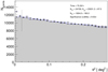 |
Fig. 3. Distribution of θ 2, the squared angular distance between the reconstructed arrival direction of individual events and the nominal source position (points) or background estimation region (gray filled area) for MAGIC observations of PKS 1510–089. The dashed line shows the value of the θ 2 up to which the significance of the detection (see the inset text) is calculated. |
2.3. Swift-XRT
Since 2006, the source is monitored in the X-ray band by the XRT instrument on board the Neil Gehrels Swift Observatory (XRT, Burrows et al. 2004). In total, 243 raw images are publicly available in SWIFTXRLOG (Swift-XRT Instrument, Log)5. From these images we selected 17 based on the simultaneity to the GeV low-flux state and contemporaneousness with MAGIC observations. The standard Swift-XRT analysis6 is described in detail in Evans et al. (2009). The data are processed following the procedure described by Fallah Ramazani et al. (2017), assuming a fixed equivalent Galactic hydrogen column density nH = 6.89 × 1020 cm−2 reported by Kalberla et al. (2005). We defined the source region as a circle of 20 pixels (∼47”) centered on the source, and a background region as a ring also centered on the source with inner and outer radii of 40 (∼94”) and 80 pixels (∼188”), respectively.
In order to calculate the average low-state X-ray spectrum of PKS 1510–089 we have combined all selected individual Swift-XRT pointings (see the blue points in Fig. 1), adding up to a total exposure of 30 ks. The 2–10 keV flux measured during those 17 pointings shows clear variability. Fitting the flux with a constant value yields χ2/Nd.o.f. = 84/16; however, the amplitude of the variability is moderate (the rms of the points is about ∼30% of the mean flux). The average spectrum is well fitted ( χ2/Nd.o.f. = 187.7/214) with a power law with an index of 1.382 ± 0.020 and  . The spectral index does not show significant variability (fit to constant yields χ2/Nd.o.f. = 31.19/16, which translates to a chance probability of ∼1.2%). A harder-when-brighter trend is only hinted at, with a Pearson’s rank coefficient for a linear correlation between flux and spectral index of 0.81 (2–10 keV) and 0.74 (0.3–10 keV).
2.4. Optical observations
PKS 1510–089 is regularly monitored as part of the Tuorla blazar monitoring program7 in the R band using a 35 cm Celestron telescope attached to the KVA (Kunglinga Vetenskapsakademi) telescope located at La Palma. The monitoring covers the period of 2012–2017 and the observations were mostly contemporaneous with the MAGIC observations of the source. The data analysis was performed with the semi-automatic pipeline using the standard analysis procedures (Nilsson et al., in prep.). The differential photometry was performed using the comparison star magnitudes from Villata et al. (1997).
Calar Alto data were acquired as part of the Monitoring AGN with Polarimetry at the Calar Alto 2.2m Telescope (MAPCAT) project8; see Agudo et al. (2012). The MAPCAT data presented here were reduced following the procedure explained in Jorstad et al. (2010).
Additionally, we used the publicly available data in the R band from the Small and Moderate Aperture Research Telescope System (SMARTS) instrument located at Cerro Tololo Interamerican Observatory (CTIO) in Chile (Bonning et al. 2012), processed as described in Ahnen et al. (2017a).
The KVA, MAPCAT, and SMARTS R-band data have been corrected for Galactic extinction using AR = 0.217 (Schlafly & Finkbeiner 2011). In the optical range, PKS 1510–089 shows mostly low emission throughout 2012–2014 and during 2017. Strong flares are seen in 2015 and 2016 at the times of high GeV state. The individual measurements performed in the optical range have very small statistical uncertainties, well below the variability observed during the selected low-state nights. Therefore, for the modeling, we use the average optical flux from 53 nights of observations (47 nights of observations with KVA, 3 with MAPCAT, and 13 with SMARTS). We take as the uncertainty the rms spread of the measurements. By applying such a procedure, we obtain that the mean optical flux during the low state is 1.55 ± 0.57 mJy. In band B we combine Swift-UVOT data (see the next section) with the SMARTS data, bringing the total number of observing nights to 20 and average flux of 1.22 ± 0.46 mJy.
2.5. Swift-UVOT
The Ultraviolet/Optical Telescope (UVOT, Poole et al. 2008) is an instrument on board the Swift satellite operating in the 180–600 nm wavelength range. The source counts were extracted from a circular region centered on the source with 5” radius, the background counts from an annular region centered on the source with inner and outer radius of 15” and 25”, respectively. The data calibration was done following Raiteri et al. (2010), where the effective wavelength, counts-to-flux conversion factor, and Galactic extinction for each filter were calculated in an iterative procedure by taking into account the filter’s effective area and the source’s spectral shape. The Galactic extinction values derived from the re-calibration procedure are Av = 0.28 mag, Ab = 0.37 mag, Au = 0.44 mag, Aw1 = 0.63 mag, Am2 = 0.78 mag, and Aw2 = 0.74 mag. The variability of the UV flux during the low-state nights is minor. The average flux of the quiescent state was derived in the same way as for the optical data. The number of quasi-simultaneous UVOT observations, contemporaneous to MAGIC observations during the Fermi-LAT low gamma-ray state is 9–13, depending on the filter.
2.6. Infrared
We use infrared observations of PKS 1510–089 performed with the REM (Rapid Eye Mount, Zerbi et al. 2001; Covino et al. 2004) 60 cm diameter telescope located at La Silla, Chile. The observations were performed with J, H, and Ks filters, with individual exposures ranging from 12 s to 30 s. After calibration using neighboring stars, the magnitudes were converted to fluxes using the zero magnitude fluxes from Mead et al. (1990). Additionally, we used the publicly available data in the J and K bands from SMARTS (Bonning et al. 2012), processed as described in Ahnen et al. (2017a).
Since the data were taken independently from MAGIC, a limited number of nights of MAGIC observations have quasi-simultaneous REM or SMARTS data. The data taken during the times classified as low state consist of five nights of REM data for H filter and 13 nights of REM or SMARTS data from J and K filters. Moreover, one of the nights observed by SMARTS on MJD 57181 had a major IR flare where the flux increased by a factor of ∼5–6 with respect to the average flux value of the rest of the selected data. We nevertheless apply the same procedure as for R-band KVA data, averaging the IR flux over these low-state observations, neglecting however the night of the IR flare. We obtain FK = 7.3 ± 2.7 mJy, FH = 4.2 ± 2.4 mJy, FJ = 2.3 ± 1.0 mJy. Including the night of the IR flare in the sample would change the FJ and FK fluxes relatively mildly (∼30% increase); however, it would increase the rms considerably to a value comparable to the flux.
2.7. Radio
We use radio monitoring observations of PKS 1510–089 performed by OVRO (15 GHz, Richards et al. 2011), Metsähovi (37 GHz, Teraësranta et al. 1998), and POLAMI (86 GHz, 229 GHz). We also use CARMA data taken at 95 GHz between August 2012 and November 2014 (Ramakrishnan et al. 2016).
Polarimetric Monitoring of AGN at Millimetre Wavelengths (POLAMI9; Agudo et al. 2018a,b; Thum et al. 2018) is a long-term program to monitor the polarimetric properties (Stokes I, Q, U, and V) of a sample of ∼40 bright AGN at 3.5 and 1.3 millimeter wavelengths with the IRAM 30m Telescope near Granada, Spain. The program has been running since October 2006, and it currently has a time sampling of ∼2 weeks. The XPOL polarimetric observing setup has been routinely used as described in Thum et al. (2008) since the start of the program. The reduction and calibration of the POLAMI data presented here are described in detail in Agudo et al. (2010, 2014, 2018a).
The 37 GHz observations were made with the 13.7 m diameter Aalto University Metsähovi radio telescope10, which is a radome enclosed Cassegrain-type antenna situated in Finland. The measurements were made with a 1 GHz band dual beam receiver centered at 36.8 GHz. The High Electron Mobility Pseudomorphic Transistor (HEMPT) front end operates at room temperature. The observations are Dicke switched ON–ON observations, alternating between the source and the sky in each feed horn. A typical integration time to obtain one flux density data point is between 1200 and 1800 s. The detection limit of the telescope at 37 GHz is on the order of 0.2 Jy under optimal conditions. Data points with a signal-to-noise ratio < 4 are considered non-detections. The flux density calibration is set by observations of the HII region DR 21. The sources NGC 7027, 3C 274, and 3C 84 are used as secondary calibrators. A detailed description of the data reduction and analysis is given in Teraësranta et al. (1998). The error estimate in the flux density includes the contribution from the measurement rms and the uncertainty of the absolute calibration.
The Owens Valley Radio Observatory (OVRO) 40 m telescope uses off-axis dual-beam optics and a cryogenic receiver with 3 GHz bandwidth centered at 15 GHz. Atmospheric and ground contributions as well as gain fluctuations are removed with the double switching technique (Readhead et al. 1989), where the observations are conducted in an ON-ON fashion so that one of the beams is always pointed on the source. Until May 2014 the two beams were rapidly alternated using a Dicke switch. Since then a new pseudo-correlation receiver has replaced the old one, and a 180° phase switch is used. Relative calibration is obtained with a temperature-stable noise diode to compensate for gain drifts. The primary flux density calibrator for those observations was 3C 286 with an assumed value of 3.44 Jy (Baars et al. 1977), while DR21 is used as a secondary calibrator source. Details of the observation and data reduction procedures are given in Richards et al. (2011).
The radio flux at all frequencies shows slow variability, not simultaneous with the flares observed at higher energies. In order to obtain the average emission during the low gamma-ray state we apply the same procedure as for the R-band flux; however, we apply a larger margin in time, using the data within ±3 days from the MAGIC observations during low Fermi-LAT flux. We obtain F15 GHz = 4.4 ± 1.2 Jy (average over 22 observations), F37 GHz = 3.9 ± 1.1 Jy (59 observations), F86 GHz = 3.14 ± 0.86 Jy (6 observations), F95 GHz = 2.16 ± 0.13 Jy (9 observations), and F229 GHz = 1.76 ± 0.42 Jy (4 observations).
3. Low gamma-ray state of PKS 1510–089
The low-state spectrum of PKS 1510–089 observed by the MAGIC telescopes was reconstructed between 63 and 430 GeV and is shown in Fig. 4. The observed spectrum can be described by a power law: dN/dE = (4.66 ± 0.59stat)×10−11(E/175 GeV)−3.97 ± 0.23stat cm−2 s−1 TeV−1. Correcting for the absorption due to the interaction with the extragalactic background light (EBL) according to Domínguez et al. (2011), we obtain the following intrinsic spectrum: dN/dE = (7.9 ± 1.1stat)×10−11(E/175 GeV)−3.26 ± 0.30stat cm−2 s−1 TeV−1. Since the excess to residual background ratio is on the order of 6%, the systematic uncertainty on the flux normalization (without the effect of the energy scale) is ±20%, larger than for typical MAGIC observations (Aleksić et al. 2016b). Also, the systematic uncertainty on the spectral slope is increased by the low excess-to-residual background ratio and, following the prescription in Sect. 5.1 in Aleksić et al. (2016b), can be estimated as ±0.4. The uncertainty of the energy scale is ±15%. Compared with previous measurements, the high-state detection in 2012 (Aleksić et al. 2014) gives a ∼1.7 times larger flux than the low state studied here. On the other hand, the most luminous flare observed from PKS 1510–089 in May 2016 gives a flux that is ∼40–80 times higher than the low state (for the MAGIC and H.E.S.S. observation window, respectively; see Zacharias et al. 2017b). Interestingly, the intrinsic spectral index of −3.26 ± 0.30stat is consistent within the uncertainties with that obtained during the high state in the 2012 (−2.5 ± 0.6stat, Aleksić et al. 2014), the 2015 flare (−3.17 ± 0.80stat, Ahnen et al. 2017a) and the 2016 flare (−2.9 ± 0.2stat, −3.37 ± 0.09stat, Zacharias et al. 2017b).
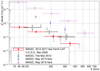 |
Fig. 4. Spectral energy distribution (SED) of PKS 1510–089 during the low state (red filled points and shaded magenta region) compared to historical measurements (open symbols): high state in March 2009 (gray stars, H.E.S.S. Collaboration 2013), high state in February–March 2012 (black diamonds, Aleksić et al. 2014), flare in May 2015 (blue crosses, Ahnen et al. 2017a), and flare in May 2016 (magenta squares, Zacharias et al. 2017b). The spectra are not deabsorbed from the EBL extinction. |
As reported in Sect. 2, the IR to UV low-state data show variability at the level of ∼40%. We search for possible variability in the MAGIC data taken during the defined low state by computing light curves using different binnings (see Fig. 5). Both the daily ( χ2/Nd.o.f. = 51.9/74) and yearly (χ2/Nd.o.f. = 3.08/5) light curves do not show any evidence of variability when fitted with a constant flux model. The gamma-ray flux of PKS 1510–089 during the low state is, however, too weak for probing variability with a similar relative amplitude at GeV energies with MAGIC or Fermi-LAT as observed in IR-UV. The average emission of the low state above 150 GeV is (4.27 ± 0.61stat)×10−12 cm−2 s−1, which is also below the all-time average of the H.E.S.S. observations ((5.5 ± 0.4stat)×10−12 cm−2 s−1, Zacharias et al. 2017a).
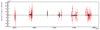 |
Fig. 5. Light curve of PKS 1510–089 obtained with MAGIC observations during the low state in daily (red thin lines) and yearly (black thick lines) binning. For clarity three nights with short exposure (resulting in flux estimation uncertainty > 15 × 10−12 cm−2 s−1) are omitted from the plot. |
4. Modeling
The multiwavelength SED constructed from the data selected according to the low flux above 1 GeV, taken between 2012 and 2017, is shown in Fig. 6. We model the broadband emission using an external Compton scenario (see, e.g., Sikora et al. 1994; Ghisellini et al. 2010) in which the gamma-ray emission is produced due to inverse Compton scattering of a radiation field external to the jet by electrons located in an emission region inside the jet. We use a particular scenario applied previously to model a high state and a flare from PKS 1510–089 (Aleksić et al. 2014; Ahnen et al. 2017a), with the external photon field being the accretion disk radiation reflected by the broad line region (BLR) and dust torus (DT).
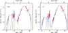 |
Fig. 6. Multiwavelength SED of PKS 1510–089 obtained from the data contemporaneous to MAGIC observations performed during Fermi-LAT low state (red points). The gray band shows the Swift-BAT 105-month average spectrum (Oh et al. 2018). Gray dot markers show the historical data from SSDC (www.asdc.asi.it). IR optical and UV data have been dereddened, MAGIC data have been corrected for the absorption by the EBL according to Domínguez et al. (2011) model. Observed MAGIC spectral points are shown in cyan. The green short-long-dashed curve shows the synchrotron component, and orange dot-dashed curve the EC component. The SSC component is shown as a cyan dotted line. The long dashed and short dashed black lines show the dust torus and accretion disk emission, respectively. The solid blue line shows the total emission (including absorption in EBL). Left panel: close model, right panel: far model (see the text). |
We apply the same BLR and DT parameters as in Ahnen et al. (2017a), namely a radius of RBLR = 2.6 × 1017 cm and RIR = 6.5 × 1018 cm, respectively. BLR and DT reflect the fBLR = 0.1 and fDT = 0.6 (the so-called covering factor) part of the accretion disk radiation, Ldisk = 6.7 × 1045 erg s−1. The DT temperature is set to 1000 K. The emission region is located at the distance r from the base of the jet and has a radius of R. As in the model employed in Ahnen et al. (2017a), jet plasma flows through the emission region. The lack of strong variability of the low-state emission and the fact that it reaches sub-TeV energies suggests that the emission region should be beyond the BLR. At such distances the cross section of the jet is large, making it difficult to explain any short-term variability, but the absorption on the BLR radiation is negligible. We consider two scenarios for the location of the emission region: the “close” scenario with r = 7 × 1017 cm and “far” scenario with r = 3 × 1018 cm. In both cases, the dominating radiation field comes from the DT. Such distances of the emission region have been applied for modeling of the 2015 flare (Ahnen et al. 2017a) and 2012 high state (Aleksić et al. 2014) respectively. The size of the emission region R = 2 × 1016 cm (for the close scenario) and R = 3 × 1017 cm (for the far scenario) is on the order of the cross section of the jet at the distance r. Although it is not a dominant emission component, the model also calculates the synchrotron self-Compton emission of the source.
The model parameters for both scenarios are summarized and compared with earlier modeling in Table 1. However, the sets of parameters are not unique solutions for describing the low-state SED, as a certain degree of parameter degeneracy occurs in these kinds of models (see, e.g., synchrotron self-Compton (SSC) model parameters degeneracy discussed in Ahnen et al. 2017b).
Input model parameters for the EC models of PKS 1510–089 emission for the low state in close and far scenarios.
The data are compared with the model in Fig. 6. Both scenarios can reproduce relatively well the IC peak. The gamma-ray data of MAGIC and Fermi-LAT are explained as the high-energy part of the EC component, with the exception of the two highest energy Fermi-LAT points that are > 1 GeV and hence are probably underestimated by the data selection procedure (see Sect. 2.1). Swift-XRT and historical Swift-BAT data follow the rising part of the EC component (with a small contribution of the SSC process in the soft X-ray range for the close scenario). The UV data form a bump that can be explained by the direct accretion disk radiation included in the model. In the IR range, the model curve underestimates the data points, especially in the case of the far model. Among the quiescent data selected, the IR data show the highest variability. The higher IR variability might come from a separate region, not associated with the GeV gamma-ray emission region.
In such a case, the IR emission associated with the low gamma-ray state would likely be at the level closer to the low edge of the observed spread in IR fluxes (reflected in the quoted uncertainty bar in Fig. 6).
The far model can reasonably reproduce the radio observations, while the close model underestimates the data due to strong synchrotron self-absorption effects given by the compactness of the emission region. This is not surprising since the radio core observed at 15 GHz is estimated to be located 17.7 pc from the base of the jet (Pushkarev et al. 2012). Using the typical scaling of the core distance being inversely proportional to the frequency, we obtain that for the highest radio point at 229 GHz its corresponding radio core should be located at ∼1 pc. Therefore, most of the radio emission should be produced at or beyond the region considered in the far scenario. However, the magnetic field considered in the far scenario, B = 0.05 G, is an order of magnitude smaller than the magnetic field estimated from the radio observations at r = 1 pc of 0.73 G (Pushkarev et al. 2012). Larger values would result in a much smaller Compton dominance than observed in the broadband SED.
It is curious that an optical/GeV high state, a days-long flare, and the low state can all be roughly described (except of the IR data) in the framework of the same external Compton scenario without a major change of the model parameters. This suggests a common origin of the gamma-ray emission of PKS 1510–089 in different activity states, with the observed differences caused by changes in the content of the plasma flowing through the emission region11. We note, however, that the model used here is rather simple. It is natural to assume that the low-state, broadband emission is an integral part of the emission in a range of distances from the base, with the varying conditions (such as B field) along the jet, rather than originating in a single homogenous region (see, e.g., Potter & Cotter 2013).
5. Limits on the absorption of sub-TeV photons in BLR
If the emission region is located inside or close to the BLR, the gamma-ray spectrum should carry an imprint of the absorption feature on the BLR photons (Donea & Protheroe 2003). The presence or lack of such an absorption can therefore be used to constrain the location of the emission region. We use the emission-model-independent approach of Cerruti et al. (2017) to put such constraints on the location of the low-state emission region of PKS 1510–089. We first make a power-law fit to the Fermi-LAT spectrum of PKS 1510–089 in the energy range of 0.1–1 GeV, which is unbiased by the data selection. Next, we extrapolate the fit to the energy range observed by the MAGIC telescopes and apply an absorption of a factor of exp(−τ), where τ is the so-called optical depth (see Fig. 7).
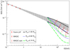 |
Fig. 7. Gamma-ray spectrum of PKS 1510–089 during low state measured by Fermi-LAT (squares) and MAGIC (filled circles). The 68% confidence band of the extrapolation of the Fermi-LAT spectrum to sub-TeV energies is shown as a gray shaded region. The extrapolation in the MAGIC energy range assuming absorption in BLR following Böttcher & Els (2016) for the emission region located at the distance of 1, 0.82, and 0.74 of the outer radius of the broad line region is shown with black solid, blue dotted, and green dashed lines, respectively. Empty circles show the effect of the systematic uncertainties on the MAGIC spectrum. |
We compare these extrapolations with the reconstructed MAGIC spectrum taking into account the statistical uncertainties as well as the systematic uncertainty both in the energy scale and in the flux normalization. The systematic uncertainties of Fermi-LAT are negligible in those calculations. Due to source intrinsic effects (e.g., intrinsic break or cutoff in the accelerated electron spectrum, the Klein–Nishina effect) the sub-TeV spectrum might be below the GeV extrapolation. Thus, no lower limit on the absorption can be derived in a model-independent way. However, it is natural to assume that there is no upturning in the photon spectrum; therefore, we can place an upper limit on the maximum absorption in the BLR. To estimate such a limit we perform a toy Monte Carlo study in which we vary 10 000 times the extrapolated Fermi-LAT flux and the measured MAGIC flux (corrected for the EBL absorption) according to their uncertainties. Next, at each investigated energy we calculate a histogram of τ(E)=ln(Fext(E)/Fobs(E)), where Fext(E) and Fobs(E) are the randomized extrapolated and randomized measured flux respectively. The limit on τ is obtained as a 95% quantile of such a distribution. We include the systematic uncertainties of MAGIC by shifting its energy scale and normalization according to their systematic limits (see empty circles in Fig. 7) and taking the least constraining one. We obtain that τ(110 GeV) < 1.4, τ(180 GeV) < 1.7, τ(290 GeV) < 2.3.
Applying a model of absorption by the BLR those limits on the optical depth can be converted to lower limits on the location of the emission region, r. We test the above procedure using two BLR models for PKS 1510–089. First, we use the optical depth calculations of Böttcher & Els (2016) assuming that 10% of the accretion disk radiation is reprocessed in the BLR. We note that Böttcher & Els (2016) assume that a homogeneous BLR in PKS 1510–089 spans between 6.9 × 1017 cm and 8.4 × 1017 cm, and reflects 10% of the disk luminosity LD = 1046 erg s−1. We obtain that the above limits result in r > 6.3 × 1017 cm (i.e., above 0.74 of the outer radius of the BLR). As an additional check we calculate the optical depths using a code adapted from Sitarek & Bednarek (2008) with the line intensities and BLR geometry of Liu & Bai (2006). We use the same radius and luminosity of the BLR as in Sect. 4. We apply however the same ratio of the outer to inner radius of BLR as in Böttcher & Els (2016), resulting in the BLR spanning from 2.34 × 1017 cm to 2.86 × 1017 cm. For such a BLR model, the limits on the optical depth obtained above force us to place the emission region farther than 3.2 × 1017 cm (i.e., beyond 1.1 of the outer radius of the BLR.
It should be noted that the method has a number of simplifications and underlying assumptions. The emission region is assumed to be relatively small compared to its distance from the black hole. This is not necessarily true, in particular for the low state emission that can be generated in a more extended region (the broad band emission modeling presented in the previous section further supports such a hypothesis). Second, if the gamma-ray emission is not produced by a single process, the spectrum can have a complicated shape (including convex). We note that for another FSRQ, B0218+357, the gamma-ray emission was explained as combination of SSC and EC process (Ahnen et al. 2016). Third, the optical depth is dependent on the assumed geometry of the BLR. For example, the size of the BLR derived in Böttcher & Els (2016) is a factor of ∼3 larger than that in Ghisellini & Tavecchio (2009). In addition, the difference between the spherical and disk-like geometry can easily change the optical depths by a factor of a few (Abolmasov & Poutanen 2017). Finally, the radial stratification of the BLR and the total fraction of the light reflected in the BLR introduce further uncertainties.
6. Conclusions
We performed the analysis of MAGIC data searching for a possible low state of VHE gamma-ray emission from PKS 1510–089. Selecting the data taken during periods when the Fermi-LAT flux above 1 GeV was below 3 × 10⁻⁸ cm−2 s−1 we collected 75 hr of MAGIC data on 76 individual nights, resulting in a significant detection of the low state of VHE gamma-ray emission. The measured flux is ∼0.6 of the flux of the source measured during high optical and GeV state (Aleksić et al. 2014) at the beginning of 2012 and ∼0.75 of the lowest previously known flux from this source (average over all the H.E.S.S. observations; Zacharias et al. 2017a). Nevertheless, the spectral shape is consistent with the previous measurements, despite a factor of 80 difference to the flux during the strongest flare observed so far from this source. This makes PKS 1510–089 the first FSRQ to be detected in a persistent low state with no hints of yearly variations in the observed flux. Future observations with the Cherenkov Telescope Array should be able to probe whether the low-state flux is also stable on shorter timescales (Acharya et al. 2013, 2017).
Previous VHE gamma-ray observations of FSRQs in flaring states suggested that the emission region during such states should be located beyond the BLR and that the emission is mostly compatible with an EC scenario. The low-state broadband emission of PKS 1510–089 from IR to VHE gamma-rays can be explained in the framework of an EC scenario, similarly to the previous VHE gamma-ray detections of the source. The presence of the sub-TeV gamma-ray emission also suggests that the emission region is located beyond the BLR where the dominating seed radiation field for the EC process is the dust torus. Comparison of the extrapolated Fermi-LAT spectrum and the MAGIC measured spectrum using two distinct BLR models allows us to put a limit on the location of the emission region beyond the 0.74 of the outer radius of BLR. The emission scenario placing the dissipation region beyond the BLR is in line with the recent studies of Costamante et al. (2018) showing that most of the Fermi-LAT detected blazars (including PKS 1510–089 ) have GeV emission consistent with lack of BLR absorption.
A fast flare observed in 2016 from PKS 1510–089 (Zacharias et al. 2017b) might nevertheless have a different origin.
Acknowledgments
We would like to thank the Instituto de Astrofísica de Canarias for the excellent working conditions at the Observatorio del Roque de los Muchachos in La Palma. The financial support of the German BMBF and MPG, the Italian INFN and INAF, the Swiss National Fund SNF, the ERDF under the Spanish MINECO (FPA2015-69818-P, FPA2012-36668, FPA2015-68378-P, FPA2015-69210-C6-2-R, FPA2015-69210-C6-4-R, FPA2015-69210-C6-6-R, AYA2015-71042-P, AYA2016-76012-C3-1-P, ESP2015-71662-C2-2-P, CSD2009-00064), and the Japanese JSPS and MEXT is gratefully acknowledged. This work was also supported by the Spanish Centro de Excelencia “Severo Ochoa” SEV-2012-0234 and SEV-2015-0548, and Unidad de Excelencia “María de Maeztu” MDM-2014-0369, by the Croatian Science Foundation (HrZZ) Project IP-2016-06-9782 and the University of Rijeka Project 13.12.1.3.02, by the DFG Collaborative Research Centers SFB823/C4 and SFB876/C3, the Polish National Research Centre grant UMO-2016/22/M/ST9/00382, and by the Brazilian MCTIC, CNPq and FAPERJ. The Fermi-LAT Collaboration acknowledges generous ongoing support from a number of agencies and institutes that have supported both the development and the operation of the LAT as well as scientific data analysis. These include the National Aeronautics and Space Administration and the Department of Energy in the United States; the Commissariat à l’Energie Atomique and the Centre National de la Recherche Scientifique/Institut National de Physique Nucléaire et de Physique des Particules in France; the Agenzia Spaziale Italiana and the Istituto Nazionale di Fisica Nucleare in Italy; the Ministry of Education, Culture, Sports, Science and Technology (MEXT), High Energy Accelerator Research Organization (KEK), and Japan Aerospace Exploration Agency (JAXA) in Japan; and the K. A. Wallenberg Foundation, the Swedish Research Council, and the Swedish National Space Board in Sweden. Additional support for science analysis during the operations phase is gratefully acknowledged from the Istituto Nazionale di Astrofisica in Italy and the Centre National d’Études Spatiales in France. This work was performed in part under DOE Contract DE-AC02-76SF00515. This paper has made use of up-to-date SMARTS optical/near-infrared light curves that are available at www.astro.yale.edu/smarts/glast/home.php. IA acknowledges support from a Ramón y Cajal grant of the Ministerio de Economía, Industria, y Competitividad (MINECO) of Spain. Acquisition and reduction of the POLAMI and MAPCAT data was supported in part by MINECO through grants AYA2010-14844, AYA2013-40825-P, and AYA2016-80889-P, and by the Regional Government of Andalucía through grant P09-FQM-4784. The POLAMI observations were carried out at the IRAM 30m Telescope. IRAM is supported by INSU/CNRS (France), MPG (Germany), and IGN (Spain). The MAPCAT observations were carried out at the German-Spanish Calar Alto Observatory, which is jointly operated by the Max-Plank-Institut für Astronomie and the Instituto de Astrofísica de Andalucía-CSIC. This research has made use of data from the OVRO 40m monitoring program (Richards et al. 2011), which is supported in part by NASA grants NNX08AW31G, NNX11A043G, and NNX14AQ89G and NSF grants AST-0808050 and AST-1109911. This publication makes use of data obtained at the Metsähovi Radio Observatory, operated by Aalto University, Finland. The authors would like to thank a number of people who provided comments to the manuscript: R. Angioni, N. MacDonald, M. Giroletti, R. Caputo, D. Thompson, and the anonymous reviewer. We would also like to thank M. Böttcher for providing us with the numerical values of the optical depths calculated in Böttcher & Els (2016).
References
- Abdo, A. A., Ackermann, M., Agudo, I., et al. 2010, ApJ, 721, 1425 [NASA ADS] [CrossRef] [Google Scholar]
- Abolmasov, P., & Poutanen, J. 2017, MNRAS, 464, 152 [NASA ADS] [CrossRef] [Google Scholar]
- Acero, F., Ackermann, M., Ajello, M., et al. 2015, ApJS, 218, 23 [Google Scholar]
- Acero, F., Ackermann, M., Ajello, M., et al. 2016, ApJS, 223, 26 [NASA ADS] [CrossRef] [EDP Sciences] [Google Scholar]
- Acharya, B. S., Actis, M., Aghajani, T., et al. 2013, Astropart. Phys., 43, 3 [Google Scholar]
- Acharya, B. S., Agudo, I., Al Samarai, I., et al. 2017, ArXiv e-prints [arXiv:1709.07997]. [Google Scholar]
- Agudo, I., Thum, C., Wiesemeyer, H., & Krichbaum, T. P. 2010, ApJS, 189, 1 [NASA ADS] [CrossRef] [Google Scholar]
- Agudo, I., Molina, S. N., Gómez, J. L., et al. 2012, Int. J. Mod. Phys. Conf. Ser., 8, 299 [CrossRef] [Google Scholar]
- Agudo, I., Thum, C., Gómez, J. L., & Wiesemeyer, H. 2014, A&A, 566, A59 [NASA ADS] [CrossRef] [EDP Sciences] [Google Scholar]
- Agudo, I., Thum, C., Molina, S. N., et al. 2018a, MNRAS, 474, 1427 [NASA ADS] [CrossRef] [Google Scholar]
- Agudo, I., Thum, C., Ramakrishnan, V., et al. 2018b, MNRAS, 473, 1850 [NASA ADS] [CrossRef] [Google Scholar]
- Ahnen, M. L., Ansoldi, S., Antonelli, L. A., et al. 2016, A&A, 595, A98 [NASA ADS] [CrossRef] [EDP Sciences] [Google Scholar]
- Ahnen, M. L., Ansoldi, S., Antonelli, L. A., et al. 2017a, A&A, 603, A29 [NASA ADS] [CrossRef] [EDP Sciences] [Google Scholar]
- Ahnen, M. L., Ansoldi, S., Antonelli, L. A., et al. 2017b, A&A, 603, A31 [NASA ADS] [CrossRef] [EDP Sciences] [Google Scholar]
- Aleksić, J., Ansoldi, S., Antonelli, L. A., et al. 2014, A&A, 569, A46 [NASA ADS] [CrossRef] [EDP Sciences] [Google Scholar]
- Aleksić, J., Ansoldi, S., Antonelli, L. A., et al. 2016a, Astropart. Phys., 72, 61 [NASA ADS] [CrossRef] [Google Scholar]
- Aleksić, J., Ansoldi, S., Antonelli, L. A., et al. 2016b, Astropart. Phys., 72, 76 [NASA ADS] [CrossRef] [Google Scholar]
- Atwood, W. B., Abdo, A. A., Ackermann, M., et al. 2009, ApJ, 697, 1071 [NASA ADS] [CrossRef] [Google Scholar]
- Baars, J. W. M., Genzel, R., Pauliny-Toth, I. I. K., & Witzel, A. 1977, A&A, 61, 99 [NASA ADS] [Google Scholar]
- Bonning, E., Urry, C. M., Bailyn, C., et al. 2012, ApJ, 756, 13 [NASA ADS] [CrossRef] [Google Scholar]
- Böttcher, M., & Els, P. 2016, ApJ, 821, 102 [NASA ADS] [CrossRef] [Google Scholar]
- Brown, A. M. 2013, MNRAS, 431, 824 [Google Scholar]
- Burrows, D. N., Hill, J. E., Nousek, J. A., et al. 2004, Proc. SPIE, 5165, 201 [NASA ADS] [CrossRef] [Google Scholar]
- Cerruti, M., Lenain, J. P., Prokoph, H., & H.E.S.S. Collaboration 2017, Int. Cosmic Ray Conf., 35, 627 [Google Scholar]
- Costamante, L., Cutini, S., Tosti, G., Antolini, E., & Tramacere, A. 2018, MNRAS, 477, 4749 [NASA ADS] [CrossRef] [Google Scholar]
- Covino, S., Stefanon, M., Sciuto, G., et al. 2004, Proc. SPIE, 5492, 1613 [NASA ADS] [CrossRef] [Google Scholar]
- Domínguez, A., Primack, J. R., Rosario, D. J., et al. 2011, MNRAS, 410, 2556 [NASA ADS] [CrossRef] [Google Scholar]
- Donea, A.-C., & Protheroe, R. J. 2003, Astropart. Phys., 18, 377 [Google Scholar]
- Evans, P. A., Beardmore, A. P., Page, K. L., et al. 2009, MNRAS, 397, 1177 [NASA ADS] [CrossRef] [Google Scholar]
- Fallah Ramazani, V., Lindfors, E., & Nilsson, K. 2017, A&A, 608, A68 [NASA ADS] [CrossRef] [EDP Sciences] [Google Scholar]
- Ghisellini, G., & Tavecchio, F. 2009, MNRAS, 397, 985 [NASA ADS] [CrossRef] [Google Scholar]
- Ghisellini, G., Tavecchio, F., Foschini, L., et al. 2010, MNRAS, 402, 497 [NASA ADS] [CrossRef] [Google Scholar]
- H.E.S.S. Collaboration (Abramowski, A., et al.) 2013, A&A, 554, A107 [NASA ADS] [CrossRef] [EDP Sciences] [Google Scholar]
- Jorstad, S. G., Marscher, A. P., Larionov, V. M., et al. 2010, ApJ, 715, 362 [NASA ADS] [CrossRef] [Google Scholar]
- Kalberla, P. M. W., Burton, W. B., Hartmann, D., et al. 2005, A&A, 440, 775 [NASA ADS] [CrossRef] [EDP Sciences] [Google Scholar]
- Liller, M. H., & Liller, W. 1975, ApJ, 199, L133 [NASA ADS] [CrossRef] [Google Scholar]
- Liu, H. T., & Bai, J. M. 2006, ApJ, 653, 1089 [NASA ADS] [CrossRef] [Google Scholar]
- Marscher, A. P., Jorstad, S. G., Larionov, V. M., et al. 2010, ApJ, 710, L126 [NASA ADS] [CrossRef] [Google Scholar]
- Mattox, J. R., Bertsch, D. L., Chiang, J., et al. 1996, ApJ, 461, 396 [NASA ADS] [CrossRef] [Google Scholar]
- Mead, A. R. G., Ballard, K. R., Brand, P. W. J. L., et al. 1990, A&AS, 83, 183 [Google Scholar]
- Oh, K., Koss, M., Markwardt, C. B., et al. 2018, ApJS, 235, 4 [NASA ADS] [CrossRef] [Google Scholar]
- Poole, T. S., Breeveld, A. A., Page, M. J., et al. 2008, MNRAS, 383, 627 [NASA ADS] [CrossRef] [Google Scholar]
- Potter, W. J., & Cotter, G. 2013, MNRAS, 429, 1189 [NASA ADS] [CrossRef] [Google Scholar]
- Prince, R., Majumdar, P., & Gupta, N. 2017, ApJ, 844, 62 [NASA ADS] [CrossRef] [Google Scholar]
- Pushkarev, A. B., Hovatta, T., Kovalev, Y. Y., et al. 2012, A&A, 545, A113 [NASA ADS] [CrossRef] [EDP Sciences] [Google Scholar]
- Raiteri, C. M., Villata, M., Bruschini, L., et al. 2010, A&A, 524, A43 [NASA ADS] [CrossRef] [EDP Sciences] [Google Scholar]
- Ramakrishnan, V., Hovatta, T., Tornikoski, M., et al. 2016, MNRAS, 456, 171 [NASA ADS] [CrossRef] [Google Scholar]
- Readhead, A. C. S., Lawrence, C. R., Myers, S. T., et al. 1989, ApJ, 346, 566 [NASA ADS] [CrossRef] [Google Scholar]
- Richards, J. L., Max-Moerbeck, W., Pavlidou, V., et al. 2011, ApJS, 194, 29 [NASA ADS] [CrossRef] [Google Scholar]
- Saito, S., Stawarz, Ł., Tanaka, Y. T., et al. 2013, ApJ, 766, L11 [NASA ADS] [CrossRef] [Google Scholar]
- Schlafly, E. F., & Finkbeiner, D. P. 2011, ApJ, 737, 103S [NASA ADS] [CrossRef] [Google Scholar]
- Sikora, M., Begelman, M. C., & Rees, M. J. 1994, ApJ, 421, 153 [NASA ADS] [CrossRef] [Google Scholar]
- Sitarek, J., & Bednarek, W. 2008, MNRAS, 391, 624 [NASA ADS] [CrossRef] [Google Scholar]
- Tanner, A. M., Bechtold, J., Walker, C. E., Black, J. H., & Cutri, R. M. 1996, AJ, 112, 62 [NASA ADS] [CrossRef] [Google Scholar]
- Teraësranta, H., Tornikoski, M., Mujunen, A., et al. 1998, A&AS, 132, 305 [NASA ADS] [CrossRef] [EDP Sciences] [Google Scholar]
- Thum, C., Wiesemeyer, H., Paubert, G., Navarro, S., & Morris, D. 2008, PASP, 120, 777 [NASA ADS] [CrossRef] [Google Scholar]
- Thum, C., Agudo, I., Molina, S. N., et al. 2018, MNRAS, 473, 2506 [NASA ADS] [CrossRef] [Google Scholar]
- Villata, M., Raiteri, C. M., Ghisellini, G., et al. 1997, A&AS, 121, 119 [NASA ADS] [CrossRef] [EDP Sciences] [Google Scholar]
- Zacharias, M., Böttcher, M., Chakraborty, N., et al. 2017a, AIP Conf. Proc., 1792, 050023 [CrossRef] [Google Scholar]
- Zacharias, M., Sitarek, J., Dominis Prester, D., et al. 2017b, Int. Cosmic Ray Conf., 35, 655 [NASA ADS] [CrossRef] [Google Scholar]
- Zanin, R., Carmona, E., Sitarek, J., et al. 2013, Proc. 33rd ICRC, Rio de Janeiro, Brazil, 773, [Google Scholar]
- Zerbi, R. M., Chincarini, G., Ghisellini, G., et al. 2001, Astron. Nachr., 322, 275 [NASA ADS] [CrossRef] [Google Scholar]
Appendix A: Data selection tests
As discussed in Sect. 2.1, the energy threshold of 1 GeV used for the selection was motivated by its proximity to the VHE energy range. However, the daily estimation of the flux above 1 GeV has a large uncertainty that can in principle affect the data selection. To test this effect we applied instead a cut to select nights with flux above 100 MeV measured by Fermi-LAT to be below 10−6 cm−2 s−1. This cut results in the same number of the MAGIC observations nights (76) selected for the low-state analysis. The number of individual nights that would change the classification to the low state or to the high state with such a cut is 9 (corresponding to 12% of the low-state sample) each. We tested the validity of the low-state data selection procedure used here by applying a cut at the flux above 100 MeV instead of 1 GeV. We therefore conclude that the value of the Fermi-LAT analysis threshold does not have a large impact on the selection of nights used for this analysis. We tested the effect of leaving the spectral index free in the light curve analysis, and found that this does not strongly affect the fraction of the data which is classified as low GeV state, following the definition described above. Fixing the spectral index to the average value of 2.36 (see the 3FGL catalog, Acero et al. 2015) would change the number of nights assigned to the low state and high state by ≲1% each.
All Tables
Input model parameters for the EC models of PKS 1510–089 emission for the low state in close and far scenarios.
All Figures
|
Fig. 1. Multiwavelength light curve of PKS 1510–089 between 2012 and 2017. From top to bottom panels: Fermi-LAT flux above 1 GeV; Swift-XRT flux 2–10 keV; U band flux from UVOT; KVA, SMARTS and MAPCAT optical flux in R-band; IR flux from REM and SMARTS in J band; radio 229 GHz flux measured by POLAMI; radio 37 GHz flux measured by Metsähovi; 15 GHz flux measured by OVRO. The red points show the observations within 12 h (or 3 days for the radio measurements) when MAGIC data have been taken during the time that Fermi-LAT flux is above 3 × 10⁻⁸ cm−2 s−1, while the blue points are observations in time bins with Fermi-LAT flux below this flux value (i.e., the low-state sample). IR, optical and UV data have been dereddened using Schlafly & Finkbeiner (2011). |
| In the text | |
|
Fig. 2. Distribution of flux above 1 GeV measured with Fermi-LAT in 30-day (thick line) or 1-day (thin line) bins. The vertical dashed line shows the value of the cut separating the low state. |
| In the text | |
|
Fig. 3. Distribution of θ 2, the squared angular distance between the reconstructed arrival direction of individual events and the nominal source position (points) or background estimation region (gray filled area) for MAGIC observations of PKS 1510–089. The dashed line shows the value of the θ 2 up to which the significance of the detection (see the inset text) is calculated. |
| In the text | |
|
Fig. 4. Spectral energy distribution (SED) of PKS 1510–089 during the low state (red filled points and shaded magenta region) compared to historical measurements (open symbols): high state in March 2009 (gray stars, H.E.S.S. Collaboration 2013), high state in February–March 2012 (black diamonds, Aleksić et al. 2014), flare in May 2015 (blue crosses, Ahnen et al. 2017a), and flare in May 2016 (magenta squares, Zacharias et al. 2017b). The spectra are not deabsorbed from the EBL extinction. |
| In the text | |
|
Fig. 5. Light curve of PKS 1510–089 obtained with MAGIC observations during the low state in daily (red thin lines) and yearly (black thick lines) binning. For clarity three nights with short exposure (resulting in flux estimation uncertainty > 15 × 10−12 cm−2 s−1) are omitted from the plot. |
| In the text | |
|
Fig. 6. Multiwavelength SED of PKS 1510–089 obtained from the data contemporaneous to MAGIC observations performed during Fermi-LAT low state (red points). The gray band shows the Swift-BAT 105-month average spectrum (Oh et al. 2018). Gray dot markers show the historical data from SSDC (www.asdc.asi.it). IR optical and UV data have been dereddened, MAGIC data have been corrected for the absorption by the EBL according to Domínguez et al. (2011) model. Observed MAGIC spectral points are shown in cyan. The green short-long-dashed curve shows the synchrotron component, and orange dot-dashed curve the EC component. The SSC component is shown as a cyan dotted line. The long dashed and short dashed black lines show the dust torus and accretion disk emission, respectively. The solid blue line shows the total emission (including absorption in EBL). Left panel: close model, right panel: far model (see the text). |
| In the text | |
|
Fig. 7. Gamma-ray spectrum of PKS 1510–089 during low state measured by Fermi-LAT (squares) and MAGIC (filled circles). The 68% confidence band of the extrapolation of the Fermi-LAT spectrum to sub-TeV energies is shown as a gray shaded region. The extrapolation in the MAGIC energy range assuming absorption in BLR following Böttcher & Els (2016) for the emission region located at the distance of 1, 0.82, and 0.74 of the outer radius of the broad line region is shown with black solid, blue dotted, and green dashed lines, respectively. Empty circles show the effect of the systematic uncertainties on the MAGIC spectrum. |
| In the text | |
Current usage metrics show cumulative count of Article Views (full-text article views including HTML views, PDF and ePub downloads, according to the available data) and Abstracts Views on Vision4Press platform.
Data correspond to usage on the plateform after 2015. The current usage metrics is available 48-96 hours after online publication and is updated daily on week days.
Initial download of the metrics may take a while.