| Issue |
A&A
Volume 619, November 2018
|
|
|---|---|---|
| Article Number | A44 | |
| Number of page(s) | 17 | |
| Section | Astrophysical processes | |
| DOI | https://doi.org/10.1051/0004-6361/201833024 | |
| Published online | 01 November 2018 | |
Subcritical transition to turbulence in accretion disc boundary layer
Sternberg Astronomical Institute, Moscow M.V. Lomonosov State University, Universitetskij pr., 13, Moscow, 119234 Russia
e-mail: This email address is being protected from spambots. You need JavaScript enabled to view it.
Received:
14
March
2018
Accepted:
1
August
2018
Abstract
Context. Enhanced angular momentum transfer through the boundary layer near the surface of weakly magnetised accreting star is required in order to explain the observed accretion timescales in low-mass X-ray binaries, cataclysmic variables, or young stars with massive protoplanetary discs. The accretion disc boundary layer is locally represented by incompressible homogeneous and boundless flow of the cyclonic type, which is linearly stable. Its non-linear instability at the shear rates of the order of the rotational frequency remains an issue.
Aims. We put forward a conjecture that hydrodynamical subcritical turbulence in such a flow is sustained by the non-linear feedback from essentially three-dimensional vortices, which are generated by quasi-two-dimensional trailing shearing spirals grown to high amplitude via the swing amplification. We refer to those three-dimensional vortices as cross-rolls, since they are aligned in the shearwise direction in contrast to streamwise rolls generated by the anti-lift-up mechanism in rotating shear flow on the Rayleigh line.
Methods. Transient growth of cross-rolls is studied analytically and further confronted with direct numerical simulations (DNS) of the dynamics of non-linear perturbations in the shearing box approximation.
Results. A substantial decrease of transition Reynolds number RT is revealed as one changes a cubic box to a tall box. DNS performed in a tall box show that RT as a function of shear rate accords with the line of constant maximum transient growth of cross-rolls. The transition in the tall box has been observed until the shear rate is three times higher than the rotational frequency, when RT ∼ 50 000.
Conclusions. Assuming that the cross-rolls are also responsible for turbulence in the Keplerian flow, we estimate R T ≲ 108 in this case. Our results imply that non-linear stability of Keplerian flow should be verified by extending turbulent solutions found in the cyclonic regime across the solid-body line rather than entering a quasi-Keplerian regime from the side of the Rayleigh line. The most favourable shear rate to test the existence of turbulence in the quasi-Keplerian regime may be sub-Keplerian and equal approximately to 1/2.
Key words: hydrodynamics / accretion, accretion disks / instabilities / turbulence / protoplanetary disks
© ESO 2018
1. Introduction
Rotating boundary layers are believed to exist in the vicinity of weakly magnetised stars accumulating the material from an accretion disc. A slowly spinning star surface causes transformation of the rotational energy of the disc into thermal energy inside the boundary layer. Thus, the boundary layer is expected to have a brightness comparable to that of the accretion disc and be the main source of radiation in a relatively higher frequency band than the disc itself. The structure of the boundary layer and the adjacent disc inner part must be determined together (see Bisnovatyi-Kogan 1994). A number of boundary layer models have been developed for various classes of objects. Usually they employ slim disc equations (Abramowicz et al. 1988) in order to match consistently the disc inner part to the boundary layer. Among them the accreting pre-main sequence stars were studied by Popham et al. (1993), whereas the accreting white dwarfs and neutron stars were studied by Narayan & Popham (1993) and Popham & Sunyaev (2001). In the latter case, the formation of a spreading layer is also possible in systems with high enough accretion rate, as was suggested by Inogamov & Sunyaev (1999).
Just as for the formation of an accretion disc, the cornerstone of boundary layer formation is the origin of effective shear viscosity providing enhanced angular momentum and mass transfer onto the star surface. Conventionally, it is parametrised by α, which is the kinematic viscosity coefficient scaled by the speed of sound and pressure radial scaleheight (see Shakura & Sunyaev 1988). This variant of viscosity prescription is similar to what is done in the disc models, where α is scaled by the disc thickness (see Shakura & Sunyaev 1973). However, the physical process veiled by an effective viscosity as well as magnitude of α remains a matter of debate, probably, to a greater extent, in the case of boundary layer rather than in the case of accretion disc. Turbulence is known to be a natural solution to this issue, but its simple (supercritical) variant is discarded by the centrifugal stability of the rotating shear flows, which represent both accretion discs and boundary layers. A “magic wand” working in hot magnetised discs, where angular velocity Ω decreases with distance to the rotation axis r, is a magnetorotational instability. However, it does not work if dΩ2/dr > 0, which is the case for the boundary layers. Such flows are locally linearly stable even in the presence of the magnetic field. In this context, an alternative mechanism of angular momentum transfer has been proposed by Belyaev et al. (2013) and more recently by Philippov et al. (2016). It was shown that global sonic instability of the flow associated with the presence of the star surface excites global non-axisymmetric acoustic modes, which are responsible for effective viscosity even in the absence of turbulence.
At the same time, the possibility that astrophysical boundary layers acquire the effective viscosity through the turbulence is not ruled out, since flows with shear rates including that of the order of |Ω| may be locally non-linearly unstable. Along with the hydrodynamical, non-linear stability of homogeneous Keplerian shear flow, which locally represents the accretion and protoplanetary discs, this is one of the major unresolved problems in astrophysical fluid dynamics. Below we consider both problems jointly. In order to be non-linearly unstable, such flows first require a candidate for transiently growing perturbations, which could be amplified by background shear by orders of magnitude for the Reynolds number R typical in astrophysical situations; second, in phase of high amplitude, those perturbations have to give a positive non-linear feedback to the basin of small perturbations subject to transient growth. Two of these conditions together introduce what is usually called a bypass scenario for transition to turbulence.
The bypass scenario is best developed in application to plane shear flows and, in particular, to the Couette flow (see Hamilton et al. (1995) and Waleffe (1997), who proposed a non-linear mechanism sustaining the turbulence). This mechanism is called the self-sustaining process (SSP) and is sketched, for example in Fig. 1 by Waleffe (1997). The transient growth of initially small streamwise rolls produces high amplitude streamwise streaks, the process usually called lift-up effect after the work by Ellingsen & Palm (1975). As streamwise streaks modify the background velocity yielding an inflexion point in a spanwise direction, the flow becomes linearly unstable with respect to non-axisymmetric modes, which in turn regenerate streamwise rolls via non-linear interactions with each other.
However, the situation becomes less clear in centrifugally stable rotating shear flows. Let us define rotation number, which characterises a dynamical contribution of rotation to shear, RΩ = −2/q, where q = −(r/Ω)dΩ/dr is the local dimensionless shear rate. Steady, non-linear self-sustaining solutions obtained in the non-rotating case, for which RΩ = 0, can be non-linearly continued into both the centrifugally unstable regime, −1 < RΩ < 0 (q > 2), and the cyclonic regime with high shear rate, RΩ ≪ 1 (−q ≫ 1) (see Rincon et al. 2007). Nevertheless, this operation cannot be extended either until the centrifugally stable anti-cyclonic (or quasi-Keplerian) regime with RΩ ≤ −1 (0 < q < 2), or far into the cyclonic regime with RΩ ≲ 1 (q ≲ −1). Presumably, this takes place because the lift-up mechanism ceases to work in both cases. On the other hand, direct numerical simulations (DNS) allow us to obtain turbulent solutions until, at least, RΩ ≈ 0.3 (see Lesur & Longaretti 2005; LL05 hereafter). It is interesting to note that such a value of rotation number is far beyond the interval of small positive RΩ corresponding to a substantial transient growth of streamwise rolls (see Sect. 5.1.1 of this paper). Another notable fact is that the quasi-Keplerian regime demonstrates a strong asymmetry in comparison with the cyclonic regime. Namely, DNS show dramatic stabilisation of the quasi-Keplerian shear, as one goes away from the Rayleigh line, RΩ = −1, to smaller rotation numbers (cf. Figs. 4 and 7 of LL05; see also the earlier DNS of the quasi-Keplerian regime made by Hawley et al. 1999). We have already noted that when RΩ = −1 exactly, the lift-up mechanism does not work, however, there is an inverse process of small streamwise streaks growing into high amplitude streamwise rolls, which is called the anti-lift-up effect (see Sect. 2.3 in Rincon et al. 2008 for more detail). The regime RΩ = −1 is neutrally stable with respect to local modal perturbations, that is, the growth of streaks can be regarded as epicyclic oscillations with an infinite period. Because finite amplitude streamwise rolls of the anti-lift-up are quite different from finite amplitude streamwise streaks of the lift-up, Rincon et al. (2007) put forward several arguments that the turbulent solution should be represented by a bypass scenario other than SSP. In any case, since a bypass transition in the regime RΩ = −1 should involve the anti-lift-up mechanism, it looks natural that LL05 observed a sharp increase of the transition Reynolds number RT as one goes to RΩ < −1, in contrast to the situation with the cyclonic regime. Indeed, the streak’s growth is strongly suppressed at RΩ < −1, as it turns into epicyclic oscillations with nearly rotational frequency (see also Sect. 5.1.2 of this paper). LL05 observed a decay of initial turbulence in the ranges −∞ < RΩ < −1.03 and 0.3 < RΩ < ∞ for R ≲ 105 within a local model of the shearing box with shearing boundary conditions. A bypass scenario proposed in this work naturally resolves the issues mentioned above.
There are a number of studies that examine properties of centrifugally stable flows either experimentally or employing DNS in the framework of the Taylor-Couette problem (the flow between the coaxial corotating cylinders, see Sect. 6 of the review by Grossmann et al. 2016). Among the recent ones are Burin & Czarnocki (2012), who observed the turbulisation of the cyclonic flow at RT ∼ 105 in the case of RΩ ≈ 0.8, and Ostilla-Mónico et al. (2016), who considered the non-stationary dynamics in the same regime numerically excluding the influence of axial boundaries, which is unavoidable in the laboratory setup. At the same time, the quasi-Keplerian regime was investigated in the experiment by Schartman et al. (2012) subsequently continued by Edlund & Ji (2014), and numerically by Ostilla-Mónico et al. (2014) subsequently continued by Shi et al. (2017). All those studies demonstrated an outstanding stability of quasi-Keplerian flow with respect to finite amplitude perturbations from R ∼ 105 up to higher than R ∼ 106. Yet, this result should be accepted with a caution, because the presence of walls may prevent the onset of self-sustaining solutions inherent to the anti-cyclonic subcritical regime as was argued by Rincon et al. (2007). Additionally, let us emphasise that most of attempts to detect turbulence have been made at super-Keplerian shear rates, 3/2 < q < 2. For example, Edlund & Ji (2014) and Shi et al. (2017) used q = 1.8 and q = 5/3, respectively1. Indeed, there is a tendency to consider the shear rates starting from q = 2, which stems from the established opinion that the closer quasi-Keplerian shear is to the Rayleigh line, RΩ = −1 (q = 2), and the farther it is from the solid-body line, RΩ → −∞ (q = 0), the less stable it becomes. However, an accompanying purpose of this work is to show that the most appropriate shear rate to test the transition to turbulence in the quasi-Keplerian regime may be found in the vicinity of q = 1/2 (see Sect. 7).
Two decades ago it was established that shear flow turbulence is a result of the subtle interplay between non-normal linear dynamics of perturbations and their non-linear interaction (see for example the review by Grossmann 2000). Although the subcritical transition is in essence a loss of non-linear stability, the phase of linear, non-modal transient growth is of much importance in the general design of shear flow turbulence. Among others, this was elucidated by Henningson (1996). It was argued that (i) transient growth as linear process is the only source of energy for subcritical turbulence, (ii) transient growth must be large, that is the linear growth factor must be much greater than unity, for the transition to occur: for particular examples, the plane Couette and Poiseille flows may become turbulent at the Reynolds numbers as low as, respectively, RT ≃ 350 and 1000, when according to Butler & Farrell (1992) and Reddy & Henningson (1993) the maximum growth factor of streamwise rolls is, respectively, ≃150 and 200. Also, a number of low-dimensional models of plane shear flow employing various representations of the non-linear dynamics demonstrated qualitatively similar behaviour during the transition: substantial non-modal growth followed by the “bootstrapping” effect (Trefethen et al. 1993; see Baggett & Trefethen 1997). These authors explained threshold exponents for transition to turbulence in each case using simple arguments based on the secondary linear instability of the transient perturbation attained the high amplitude. Thus, it was shown that transient dynamics can always be distinguished in the whole loop of the sustenance of turbulence (see caption for Fig. 3 by Baggett & Trefethen 1997)).
The reasoning just mentioned makes the transient growth a pivotal process responsible for the generation of the specific high-amplitude inputs for the sequential non-linear feedback. Such high-amplitude inputs are the streamwise streaks in the case of plane shear flows, but what are they in the case of centrifugally stable homogeneous and boundless rotating shear flow? To answer this question in this paper, we (i) consider three-dimensional (3D) perturbations, which are able to exhibit large transient growth, (ii) perform a critical test, which indicates that high-amplitude perturbations generated during this transient growth have to do with the sustenance of turbulence. Issues (i) and (ii) are tackled solving, respectively, the linear problem (1)–(4) and the more general non-linear problem (53)–(55).
It is known that shear flow allows for the existence of the so-called Kelvin modes, or alternatively, shearing vortices exhibiting the transient growth via the swing amplification2 (see Chagelishvili et al. 2003). The shearing vortices are spanwise-invariant, nearly streamwise perturbations contracted by a background motion. In rotating flow, they take the form of spirals, whereas the instant of swing corresponds to the transformation of the leading spirals into trailing spirals or vice versa (see e.g. Razdoburdin & Zhuravlev 2015). Conservation of a spanwise vorticity perturbation is the physical reason for the growth of their velocity and pressure perturbations. The swing amplification is a two-dimensional (2D) process, which takes place independently of whether the shear is plane or rotating: the Coriolis force does not affect the growth of shearing vortices in contrast to previously discussed rolls and streaks. However, shearing vortices grow considerably weaker rather than rolls and streaks, since they are much more suppressed by viscosity. The swing amplification gives the kinetic energy growth by a factor ∝ R2/3, rather than ∝ R2 as in the case of lift- and anti-lift-up. Mukhopadhyay et al. (2006) estimated that R ∼ 106 is required to obtain the growth factor of shearing spirals comparable to the growth factor of rolls necessary to activate the SSP in the plane Couette flow. Remarkably, this claim is valid for both the plane and the rotating (no matter which cyclonicity) flows and does not change with the shear rate, since it can be shown that the maximum growth factor of shearing vortices Gmax ≈ R2/3exp ( − 2/3) provided that the time is measured in the inversed shear rate rather than in the inversed rotational frequency (cf. Eq. (83) by Afshordi et al. (2005) and Eq. (9) by Mukhopadhyay et al. 2005). Thus, the role of shearing vortices is negligible either at the Rayleigh line, or in absence of rotation, but as soon as RΩ is either sufficiently smaller than −1, or sufficiently larger than 0, the growth of streaks and rolls vanishes and the shearing vortices become the kind of perturbations exhibiting the largest transient growth in the flow. This picture was confirmed for a variety of models by Ioannou & Kakouris (2001), Mukhopadhyay et al. (2005), Yecko (2004), and more recently by Maretzke et al. (2014), Zhuravlev & Razdoburdin (2014), and Razdoburdin & Zhuravlev (2017) who carried out studies of the transient dynamics of linear perturbations in the quasi-Keplerian regime using rigorous optimisation methods, which allow us to obtain the optimal perturbations exhibiting the largest possible transient growth.
For very high Reynolds numbers typical in astrophysical boundary layers and the adjacent accretion discs, the growth of shearing spirals becomes quite significant. However, its role in the transition to turbulence remains unclear. On the one hand, it seems plausible that the shearing spirals are involved in 2D models of subcritical turbulence in shear flows simulated by Umurhan & Regev (2004), Johnson & Gammie (2005), and Horton et al. (2010). Furthermore, Lithwick (2007) suggested a 2D variant of positive non-linear feedback sustaining the growth of shearing spirals. He showed that the coupling between shearing spirals at the instant of swing and small-amplitude axisymmetric vortices generates a new shearing spiral capable of transient growth. On the other hand, Lithwick (2009) revealed that the streamwise scale of a shearing spiral must exceed the disc scale height to make this process work in the 3D model, otherwise the shearing spiral is destroyed by resonant interaction with a 3D axisymmetric vortex (see also the simulations by Shen et al. 2006). Consequently, it seems reasonable that shearing spirals are only relevant to 2D turbulence, which may occur at scales above the accretion disc scale height: moreover, Razdoburdin & Zhuravlev (2017) have recently confirmed that shearing spirals keep the ability for significant transient growth even when their streamwise scale is comparable to the disc global radial scale. Also, the lack of the positive 3D feedback from shearing spirals at phase of swing is indirectly confirmed by the DNS of LL05, which show that RT substantially depends on the shear rate for RΩ ≲ 1 in the cyclonic case. In turn, this means that Gmax strongly varies along the curve of RT(q). Hence, positive non-linear feedback would come into play at a different amplitude of working perturbation  for different shear rates, which would require further clarification3. Additionally, Maretzke et al. (2014) revealed a small difference between the optimal perturbations in cyclonic and quasi-Keplerian regimes of the flow between the cylinders: in the cyclonic regime, the optimals are not shearing spirals but their slightly modified counterparts with a weak spanwise dependence. Coincidently or not, the non-linear instability of the cyclonic flow between cylinders is already observed, rather than that of the quasi-Keplerian flow. To summarise, we suppose that the shearing spirals considered as spanwise invariant perturbations seem unlikely to be an ingredient of the non-linear feedback in the bypass scenario of subcritical transition to 3D turbulence on scales small compared to the disc scale height.
In this work we consider analytically the linear local dynamics of quasi-2D shearing spirals in the rotating, homogeneous, boundless, and centrifugally stable shear flow. By a quasi-2D shearing spiral, we mean a spatial Fourier harmonics (SFH) of small perturbation, which initially has a zero spanwise velocity perturbation, but a small non-zero spanwise wavenumber. Such perturbations are not optimal, meaning they do not attain the largest possible growth factor measured at the instant of swing. Instead, during the swing amplification they generate essentially 3D vortices of a new type, which we refer to as cross-rolls, since those are aligned in the shearwise direction in contrast to ordinary streamwise rolls generated via the anti-lift-up mechanism on the Rayleigh line (see Fig. 9). We show that while the “planar” eddies constructed of shearwise and streamwise velocity perturbations decay as the shearing spiral is wound back by a background flow, the cross-rolls conserve their amplitude and fade due to viscous dissipation only. The growth factor of cross-rolls with respect to the growth factor of the shearing spiral at the instant of swing is less than unity and decreases when the shear rate alters from q = −∞ up to q = 2. Thus, the cross-rolls amplitude is larger in the cyclonic regime, but smaller in the quasi-Keplerian regime. Also, it vanishes both at the solid-body line and at the Rayleigh line. We note that the growth factor of cross-rolls can be arbitrarily high provided that the initial quasi-2D shearing spiral is sufficiently tightly wound. We suggest that the non-linear instability and corresponding self-sustained turbulent solutions in the regime sufficiently far from both the centrifugally unstable interval and the non-rotating case are provided by the positive non-linear feedback associated with either a secondary linear instability of the flow containing the finite amplitude cross-rolls, or the interaction of cross-rolls with each other. Either of these two processes may generate new small quasi-2D shearing spirals capable of substantial swing amplification. Evidence for that comes from our simulations of subcritical transition to turbulence in the cyclonic regime. It turns out that in the shearing box model with periodic boundary conditions the transition is facilitated in the box stretched along the rotation axis, which indicates that perturbations with small but non-zero spanwise wavenumber are involved in that process. Indeed, the numerical domain of finite size does not affect the 2D shearing spirals while it works as an ideal high-pass filter for harmonics with non-zero spanwise wavenumbers: it completely cuts off wavelengths larger than spanwise size of the numerical domain, whereas the first wavelength smaller than this size and satisfying the periodic boundary conditions is the best resolved by the numerical scheme. The inherent “flaw” of shearing box simulations becomes the useful tool in our case: the cross-rolls with streamwise size comparable to the box streamwise size, so the least susceptible to viscous damping, are forbidden in a cubic box but allowed in a tall box. This way, in the tall box we manage to find the transition up to q = −3 (RΩ ≈ 0.67). Furthermore, we find that RT obtained in the tall box simulations corresponds approximately to the constant maximum growth factor of cross-rolls in the range q ∼ −35 ÷ −3. Supposing that the transition to self-sustained turbulence in the quasi-Keplerian regime corresponds to the same threshold growth factor of cross-rolls, we predict the transition Reynolds number for 0 < q < 2 (see Fig. 8), which is RT ≲ 108 for the Keplerian shear rate. This is consistent with the results of LL05 concerning the asymmetry of RT(q) in the vicinity of RΩ = 0 and RΩ = −1. Besides, it seems unrealistic to obtain the transition in the quasi-Keplerian regime considering the super-Keplerian shear rates. If our suggestion is true, the strategy of searching for hydrodynamical turbulence in the Keplerian flow should be changed: one should extend the turbulent solution from the cyclonic regime with high negative shear rate to the quasi-Keplerian regime across the solid-body line, RΩ = +∞ →RΩ = −∞, rather than start from a turbulent solution obtained on the Rayleigh line, which has a different origin and properties. We predict that the most favourable value of the shear rate to test the existence of hydrodynamical turbulence in the quasi-Keplerian regime is q = 1/2.
In the case of plane shear flow, RΩ = 0, SFH with arbitrary non-zero spanwise wavenumber is described by an exact analytical solution obtained by Chagelishvili et al. (2016). At the limit of zero spanwise wavenumber, quasi-2D shearing spirals turn into SFH, which are usually called shearing spirals. From now on, we omit prefix the “quasi-2D”, so that by shearing spirals we mean all SFH with initially planar velocity perturbation, which may have a small non-zero spanwise wavenumber.
2. Linear perturbations in rotating shear flow
Local vortical 3D perturbations in viscous homogeneous rotating shear flow obey the following equations:
 (1)
(1)
 (2)
(2)
 (3)
(3)
 (4)
(4)
where ux, uy, and uz are the Eulerian perturbations of velocity components, ρ0 is a constant background density, and p is the Eulerian perturbation of pressure. By definition,
and kinematic viscosity ν is assumed to be a constant. Variables x, y, and z are Cartesian coordinates, which locally correspond to radial, azimuthal, and axial directions in boundary layer (or disc), respectively, whereas Ω0 is angular velocity of fluid rotation at x = 0 corresponding to some radial distance r0 ≫ x. Also, q is a constant shear rate that defines the background azimuthal velocity as vy = −qΩ0x. Equations (1)–(4) are vertically unstratified linearised versions of small shearing box equations (see A.3 Umurhan & Regev 2004). Throughout the text, the variables x, y, z are alternatively referred to as, respectively, shearwise, streamwise, and spanwise coordinates (or directions). The shear rate is positive (negative) in the case of anti-cyclonic (cyclonic) flow. The anti-cyclonic case is usually divided into Rayleigh-stable regime 0 < q ≤ 2, also referred to as the quasi-Keplerian regime with particular q = 3/2 corresponding to the Keplerian flow, and Rayleigh-unstable regime q > 2 subject to centrifugal linear instability. The solid-body line and the Rayleigh line are represented, respectively, by q = 0 and q = 2, whereas q → ±∞ are the limits corresponding to plane shear flow. In what follows, we are interested in the whole range −∞ < q < 2.
2.1. Dimensionless equations for shearing harmonics
We consider a boundless shear, which allows us to look for the partial solutions of Eqs. (1)–(4) in the form of SFH,
 (5)
(5)
where f is any of perturbation quantities and f̂ is its Fourier amplitude specified by the dimensionless wavenumbers (kx, ky, kz). By Eq. (5) it is implied that the problem is considered with respect to the dimensionless comoving Cartesian coordinates
 (6)
(6)
where L is an auxiliary distance. Correspondingly, kx, ky, and kz are expressed in units of L−1. Let us assume from now on that ky > 0 and L is chosen in such a way that ky = 1. We omit the primes everywhere below and note that with respect to the original coordinates SFH acquires a varying radial wavenumber k̃x ≡ kx + qt. We arrive at the following dimensionless equations for SFH:
 (7)
(7)
 (8)
(8)
 (9)
(9)
 (10)
(10)
where velocities are expressed in units of Ω0L and pressure normalised by a constant background density, W ≡ p/ρ0, is expressed in units of L2Ω02. The non-zero kinematic viscosity yields a finite value of the Reynolds number
 (11)
(11)
and 
The normalisation used above is somewhat different from the accepted one (see e.g. LL05 and Mukhopadhyay et al. 2005). Specifically, the time is measured in units of Ω0−1 rather than in units of (qΩ0)−1. We choose the former variant, since it allows us to cross continuously the solid-body line.
Next, as soon as we are dealing with vortical dynamics, it is convenient to operate with equations for ûx and a shearwise component of vorticity SFH defined as ω̂ ≡ k × û:
 (12)
(12)
 (13)
(13)
 (14)
(14)
3. Production of 3D vortices by shearing spirals: inviscid dynamics
We assume throughout this section that R → ∞.
3.1. Swing amplification
Here we revisit the well-known mechanism of swing amplification of vortices, which takes place in the xy-plane. Namely, in the case ûz = 0, kz = 0, the problem (13)–(14) becomes one-dimensional and the evolution of the corresponding 2D SFH is described by a single equation
 (15)
(15)
provided that the velocity is divergence-free,
 (16)
(16)
The solution of Eq. (15) is
 (17)
(17)
where the normalisation k0 ≡ k(t = 0) is obtained from the condition of doubled kinetic energy density of 2D SFH equals to unity:
Accordingly, we have
 (18)
(18)
The perturbation of pressure behaves in the following way:
 (19)
(19)
The solution (17)–(18) conserves the spanwise component of the vorticity (see Chagelishvili et al. 2003):
 (20)
(20)
which results in the transient growth of 2D SFH in the case of leading spirals, kx < 0, for the quasi-Keplerian regime, q > 0, and in the case of trailing spirals, kx > 0, for the cyclonic regime, q < 0. Indeed, at the instant of swing, ts ≡ −kx/q, the shearwise wavenumber vanishes, k̃x = 0, and their growth factor defined as the ratio of current energy density of 2D SFH to its initial energy density reads
 (21)
(21)
For |kx|≫1 gs ≈ kx2, attaining an arbitrary high value for sufficiently wound spirals. The maximum possible gs is limited by damping due to the microscopic viscosity of the fluid and will be evaluated in Sect. 4.
3.2. Dynamics of SFH with non-zero spanwise wavenumber
Let us consider SFH with small but non-zero |kz|≪14. Without loss of generality, we assume that kz > 0 from now on. We also assume that initially SFH has a planar velocity field, that is, ûz(t = 0) = 0. Combining (10) and (12) we formulate the initial condition in the form
 (22)
(22)
It can be seen that Eq. (14) together with the initial condition Eq. (22) implies that ω̂x ~ kz, which makes the first term in the right-hand side (RHS) of Eq. (13) as small as ∼O(kz2) comparing to the second term therein. Consequently, in order to obtain the solution for 3D SFH in the leading order in kz ≪ 1, we drop the first term in the RHS of Eq. (13) going back to the 2D solution for ûx given by Eq. (15). Thus, for SFH weakly depending on the spanwise direction, ûx(t) is approximately given by Eq. (17).
Next, combining (10) and (12) we get an exact expression for ûz in terms of ûx and ω̂xand :
 (23)
(23)
Thereby, the term kzûz in the continuity Eq. (10) must be as small as ∼O(kz2) in comparison with the other two terms there. Thus, we assume that relation (16) holds for 3D SFH and ûy is approximately given by its 2D expression, (18). Of course, this implies that pressure also approximately obeys the 2D solution (19).
As we see, spanwise dynamics of 3D SFH is separated from the swing amplification dynamics described in Sect. 3.1 and ω̂x is obtained from Eq. (14) by integrating the expression (17) over the time,
![Mathematical equation: $$ \begin{aligned} \hat{\omega }_x=k_z k_0 \left[\frac{2-q}{q}\left(\arctan \tilde{k}_x-\arctan k_x\right)+\frac{k_x}{k_0^2}\right]\cdot \end{aligned} $$](/articles/aa/full_html/2018/11/aa33024-18/aa33024-18-eq28.gif) (24)
(24)
As t → ∞ and, respectively, |k̃x| → ∞, the shearwise component of the vorticity perturbation tends to a constant non-zero value. We refer to this asymptote of SFH as a “plateau” of SFH. We conclude that along with the existing “planar” eddies, a set of other vortices associated with this non-zero limit of ωx is generated as a “byproduct” of swing amplification. The latter will be referred to as “cross-rolls” in this work. The cross-rolls are directed across the stream in contrast to the streamwise rolls produced by the anti-lift-up mechanism in the flow on the Rayleigh line (see Fig. 9 and the details in Appendix A below). An important feature of the cross-rolls is that the spanwise velocity perturbation gains a non-zero value at t → ∞, whereas the velocity perturbation components associated with the planar eddies vanish like ûx ∼ O(t−2) and ûy ∼ O(t−1). Equations (17) and (24) together with the relation (23) taken in the leading order in kz ≪ 1 yield5
![Mathematical equation: $$ \begin{aligned} \hat{u}_z= k_z k_0 \left[ \frac{2-q}{q}\left(\arctan \tilde{k}_x-\arctan k_x\right) + \frac{k_x}{k_0^2}-\frac{\tilde{k}_x}{k^2}\right]\cdot \end{aligned} $$](/articles/aa/full_html/2018/11/aa33024-18/aa33024-18-eq29.gif) (25)
(25)
Thus, Eq. (25) leads to the following asymptote of ûz at t → ∞,
 (26)
(26)
As soon as the shearing spiral is wound up by the shear after the instant of swing, the ratio |ûz/ûy| increases, which implies that the cross-section of cross-rolls becomes elongated in a spanwise direction. At the same time, cross-rolls shrink along their axes, as far as the shearwise wavenumber increases. This, in turn, makes a streamwise component of the vorticity perturbation, ωy, grow linearly with time. Since
 (27)
(27)
 (28)
(28)
Equation (26) demonstrates the basic features of cross-rolls production. Clearly, their amplitude is proportional to pressure perturbation spanwise gradient at the instant of swing, which is ∝ kz|kx| (cf. Eq. (19)) at k̃x = 0. Also, it decreases as the shear rate goes from q = −∞ to q = 2 and vanishes exactly at q = 2. Those features will be illustrated below in Fig. 1, where the growth factors of shearing spirals with non-zero spanwise number will be plotted for different shear rates.
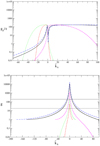 |
Fig. 1. Short-dashed, dotted, long-dashed, solid, and dot-dashed curves: gz(k̃x) (top panel) and g(k̃x) (bottom panel) for transient growth of the particular SFH at q = −5, −1.5, 0.5, 1.5, and 1.6, respectively. In each case, kx and kz are chosen in such a way that SFH attains the constant value gz(k̃x max) = gz max ≈ 180ϵ (see Sect. 3.3 for definition of ϵ). This value of gz max/ϵ is obtained employing the procedure (ii) (see this section) in order to fit the transitional dependence RT(q) found in the tall box simulations of turbulence in the cyclonic regime (see Sect. 6) for details and the dashed curve on the top panel in Figs. 6 and 8. Solid and dashed horizontal lines on the bottom panel mark the value of corresponding gz max for ϵ = 1 and ϵ = 0.1, respectively. |
3.3. Restriction on value of spanwise wavenumber
Now we are a step away from estimating the maximum value of kz = kz max, which restricts the validity of the solution for 3D SFH obtained above in the leading order in kz ≪ 1. At sufficiently large kz, the swing amplification can no longer be separated from the spanwise dynamics, which starts to destruct the shearing spiral in the xy-plane. Moreover, comparing the first term in the RHS of Eq. (13) to the second term therein, we find that these terms always become of the same order at a sufficiently large time for any small value of kz provided that the first term contains ω̂x given by Eq. (24), while the second term contains ûx given by Eq. (17). This takes place since ûx decreases as O(t−2) long after the instant of swing. We must consequently provide a restriction on kz estimating a higher order correction to the solution given in Sects. 3.1 and 3.2 at the selected period of time.
For that, let us assume that with the account of the first term in the RHS of Eq. (13), the 2D solution (17) acquires a small correction  . Substituting
into Eq. (13), we derive the following equation for û′x
![Mathematical equation: $$ \begin{aligned} \frac{\mathrm{d}}{\mathrm{d}\tilde{k}_x} ( k^2 \hat{u}_x^\prime ) = - 2k_0 \left[ \frac{2-q}{q^2} (\arctan \tilde{k}_x - \arctan k_x) + \frac{k_x}{q k_0^2} - \frac{\tilde{k}_x}{k^4} \right]\cdot \end{aligned} $$](/articles/aa/full_html/2018/11/aa33024-18/aa33024-18-eq35.gif) (29)
(29)
Given the zero initial condition û′x(t = 0) = 0, we find that
![Mathematical equation: $$ \begin{aligned} k^2 \hat{u}_x^\prime = - \frac{2k_x}{q k_0} \left( \tilde{k}_x - k_x \right) + \frac{2k_0(2-q)}{q^2} \left[\tilde{k}_x\left( \arctan k_x - \right. \right. \nonumber \\ \left. \left. \arctan \tilde{k}_x \right) + \ln \left(\frac{k}{|k_0|} \right) \right] + \frac{1}{|k_0|} - \frac{|k_0|}{k^2}\cdot \end{aligned} $$](/articles/aa/full_html/2018/11/aa33024-18/aa33024-18-eq36.gif) (30)
(30)
We estimate kz max from the assumption that it corresponds to a constant ratio of the amplitude of  and the amplitude of leading order ûx given by Eq. (17)
 (31)
(31)
where k̃x max is taken at some time after the instant of swing and corresponds to a certain location of SFH on its plateau. We note that the higher |k̃x max| is, the smaller is kz max and the longer is the duration of our analytical approximation. Most naturally, k̃x max can be evaluated at the latest extremum of ûz(t), which emerges as one incorporates viscous damping into the problem.
4. Taking viscous damping into account
Primarily, viscous force confines the swing amplification of SFH as the initial winding of the spiral and so the duration of 2D transient growth become limited by viscous dissipation. Thus, the largest value of gs corresponds to some kx = kx max. Additionally, viscous force causes damping of vertical motions and the asymptote (26) is replaced by extremum of ûz at some time after the instant of swing. Below we identify this time with k̃x = k̃x max used in Eq. (31) (see Sect. 5).
To determine both kx, max and k̃x max rigorously, let us suppose that ûx, ω̂x is the solution of Eqs. (13)–(14) obtained in the inviscid limit R → ∞. Then, the solution of the same equations taken with the account of non-zero viscosity R < ∞ is represented by
where
![Mathematical equation: $$ \begin{aligned} \gamma = \frac{1}{qR} [ (1+k_z^2) (\tilde{k}_x - k_x) + \frac{1}{3} (\tilde{k}_x^3 - k_x^3) ]. \end{aligned} $$](/articles/aa/full_html/2018/11/aa33024-18/aa33024-18-eq40.gif) (32)
(32)
For simplicity below we neglect by  in comparison with unity in (32) since kz ≲ 1 as far as q ϵ ≲ 1, which is assessed from the condition (31).
The spanwise velocity perturbation is modified in the same way:
 (33)
(33)
where ûz is given by Eq. (25). This allows one to obtain kx, max and k̃x max jointly as the roots of the set of equations
 (34)
(34)
 (35)
(35)
provided that the initial SFH is assumed to be the leading spiral (kx max < 0 and k̃x max > 0) in the quasi-Keplerian flow (q > 0) and, vice versa, the trailing spiral (kx max > 0 and k̃x max < 0) in cyclonic flow (q < 0).
4.1. The case of tightly wound SFH
In the limit of |kx max|≫1 and |k̃x max| ≫ 1, which is valid for sufficiently high R, the approximate relations

can be substituted into Eq. (25). Then, Eq. (34) simply recovers an approximate value of kx max, which follows from the estimation of Razdoburdin & Zhuravlev (2017) of maximum duration of the swing amplification tmax (see their Eq. (B2)):
 (36)
(36)
Thus, a very high transient growth of 2D SFH ∝ R2/3, and so the amplitude of the cross-rolls, can be reached taking into account that the Reynolds number may be as huge as 1010 in astrophysical boundary layers and discs.
Furthermore, Eq. (35) yields the estimation for k̃x max,
 (37)
(37)
provided that R1/2 ≫ 1.
5. Maximum growth factor of cross-rolls
The growth of the cross-rolls can be measured by energy density stored in vertical motion. In this case, since the initial condition (22) sets SFH with the unit energy and the planar velocity field, the growth factor of the cross-rolls is defined as
 (38)
(38)
Then, the quantity
 (39)
(39)
can be considered as an estimate of the largest possible amplification of cross-rolls generated by shearing spirals. We note that gz max/ϵ is the function of R and q. One may assume that violation of our analytical approximation discussed in Sect. 3.3 corresponds to the breakdown of swing amplification being a unique mechanism generating the cross-rolls. Of course, an exact kz max corresponding to the cross-rolls of the largest amplitude can be obtained solving the full set of Eqs. (13)–(14) without an expansion over kz. Nevertheless, it is known that kz max should be at least kz max ≲ |q/(2 − q)|6, as the parameter β ≳ 1 introduced by Balbus & Hawley (2006) in their Eq. (39) substantially weakens the swing amplification and, consequently, the cross-rolls amplitude. In this study, we intend to draw main conclusions assuming that Eq. (39) gives a reasonable estimate of the largest cross-rolls generated by shearing spirals, whereas their exact identification from a strict solution of (13)–(14), as well as determination of the corresponding kz max, is a subject for future studies with the use of an optimisation technique.
Below we determine the largest growth factor of cross-rolls using accurate and approximate procedures.
-
i)
An accurate determination of gz max(q, R) is done by solving Eqs. (34)–(35) numerically, which subsequently provides us with kz max from the condition (31). Then, gz max is obtained from Eq. (33) with kx = kx max, k̃x = k̃x max, and kz = kz max.
-
ii)
In the case of sufficiently high Rgz max can be estimated analytically. Indeed, as the conditions kx max ≫ 1 and k̃x max ≫ 1 are fulfilled, Eq. (30) simplifies to
and yields the following estimation for kz max
 (40)
(40)Finally, in order to estimate the largest growth factor of cross-rolls in this case, one must substitute Eqs. (36), (37), and (40) into
 (41)
(41)
Now, setting gz max/ϵ obtained according to the procedure (i) or (ii) to a constant value, we find R(q) as a root of Eq. (39). This also implies that kx max(q), k̃x max(q), and  have been determined, so that we are ready to plot the growth factors of the particular SFH corresponding to constant gz max/ϵ for several values of q (see Fig. 1). These growth factors have to be regarded as functions of time or, equivalently, k̃x: so g(k̃x) is defined by Eq. (21) and gz(k̃x) is defined by Eq. (38). As one can see on the top panel in Fig. 1, all curves of gz(k̃x) attain the same maximum value gz max/ϵ, which occurs after the instant of swing at negative and positive k̃x = k̃x max for cyclonic and quasi-Keplerian regimes, respectively. If it were not for viscous damping, gz would tend to the plateau, which has been found previously for the inviscid solution (see Eq. (26)). While comparing two panels in Fig. 1, we see that the ratio (gs/gz max)ϵ, where gs is a factor of 2D swing amplification of SFH, dramatically (and monotonically) increases as one goes from large cyclonic shear rates across the solid-body line up to the marginal case of the Rayleigh line q = 2. For example, at the Keplerian shear rate this ratio attains almost 102. Thus, the cross-rolls of the same intensity are generated by SFH with much larger |kx| as one approaches the Rayleigh line. The larger is |kx|, the tighter the winding of the initial shearing spiral is, the more it is susceptible to viscous dissipation at a typical time ∝ |kx|−2. Consequently, the closer one approaches the Rayleigh line, as starting from q = −∞, the higher the Reynolds number required in order to generate cross-rolls of the same intensity. This is reflected in the fit of our simulations of the subcritical transition to turbulence in the cyclonic regime (see Sect. 6 and solid curve on the top panel in Fig. 6) as well as in our prediction of the subcritical transition to turbulence in the quasi-Keplerian regime (see Sect. 7 and curve in Fig. 8).
Next, Fig. 2 illustrates the immediate cause of the suppression of the cross-rolls generated in the low-shear (|q|∼1) cyclonic regime and even more in the quasi-Keplerian regime in comparison with the high-shear (|q|≫1) cyclonic regime. There are the profiles of pressure perturbation amplitude as a function of k̃x plotted for shearing spirals shown in Fig. 1. For SFH these profiles also represent the behaviour of spanwise acceleration of fluid elements in the perturbed flow. At first, as the shear rate goes from −∞ up to 1/2, the net acceleration impulse in the spanwise direction decreases just because |Ŵ| in the vicinity of the instant of swing attains a smaller value. Next, at q = 1/2 the point |Ŵ|(k̃x = 0) transforms from maximum to minimum and, further, for q > 1, |Ŵ| changes sign in the vicinity of the instant of swing. Eventually, as q → 2, the net acceleration of fluid elements in positive and negative spanwise directions balance each other, so that one is left with planar velocity perturbation as the shearing spiral is wound up by the shear after the instant of swing. Certainly, an additional dip in growth of the cross-rolls, which must occur in the vicinity of the solid-body line q = 0, is imposed on the described picture. Therefore, there must exist a local maximum of growth of the cross-rolls generated by the initial SFH with constant kx and kz in the quasi-Keplerian regime. In Sect. 7 we show that this local maximum comes out through the local minimum of the transition Reynolds number occurring near the q = 1/2.
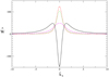 |
Fig. 2. Short-dashed, dotted, long-dashed, and solid curves: ℑ[Ŵ](k̃x) according to Eq. (19) for q = −5, −1.5, 0.5, and 1.5, respectively. The growth factors of the corresponding SFHs are shown in Fig. 1. There is no curve for q = 1.6 since it virtually coincides with the curve for q = 1.5. |
5.1. Cross-rolls in comparison with rolls and streaks
Let us estimate the growth factor of rolls generated by the anti-lift-up effect and streaks generated by the lift-up effect in centrifugally stable rotating flow. This is to be done in order to evaluate the role of those known mechanisms relative to the generation of cross-rolls discussed above.
Both lift-up and anti-lift-up mechanisms describe the transient growth of axisymmetric perturbations. Consequently, we set ky = 0 in Eqs. (7)–(10) and obtain the set of equations for ûx and ω̂x
 (42)
(42)
 (43)
(43)
in the inviscid limit R → ∞, which yields the equation for ûx
 (44)
(44)
where
with α ≡ kx/kz.
The solution of Eq. (44) reads
 (45)
(45)
where amplitude A and phase φ are to be determined from initial conditions.
Further, ω̂x is obtained with the help of Eq. (43)
 (46)
(46)
whereas
 (47)
(47)
since ω̂x = kzûy for axisymmetric perturbations. Finally,
 (48)
(48)
5.1.1. Growth of rolls
The lift-up mechanism provides the transient growth of streamwise rolls, that is, initial vortices with ûy = 0. This implies that  and
and  for perturbations with initial
  . Thus,
  and φ = π/2.
Consequently, the growth factor of rolls defined as ḡ ≡ g + gz reads
 (49)
(49)
The corresponding maximum growth factor reads
 (50)
(50)
and becomes unlimited as q → −∞, that is, in the non-rotating shear flow.
5.1.2. Growth of streaks
The anti-lift-up mechanism provides the transient growth of streamwise streaks, that is, initial vortices with ûx = 0, ûy = 1, ûz = 0. Thus, in this case ![Mathematical equation: $ A=\sqrt{2/\left[(2-q)(\alpha^2+1)\right]} $](/articles/aa/full_html/2018/11/aa33024-18/aa33024-18-eq68.gif) , φ = 0.
, φ = 0.
The growth factor of streamwise streaks is
 (51)
(51)
The corresponding maximum growth factor reads
 (52)
(52)
and becomes unlimited as q → 2, on the Rayleigh line.
Hence, the maximum transient growth factor attained through either the lift-up or anti-lift-up mechanism is independent of SFH wavenumbers. Since there is no low limit on their absolute values in the boundless shear, either the rolls or the streaks can be amplified up to ḡmax given, respectively, by Eqs. (50) and (52) at any R. At the same time, the cross-rolls cannot be amplified stronger than the value estimated by definition (39) with ûz, v substituted from Eq. (33). One can see that additionally to a constraint coming from the damping of the swing amplification, which is  , the growth of the cross-rolls is reduced by a factor of
  comparing to ḡmax. We conclude that strictly in the absence of rotation or, alternatively, on the Rayleigh line, cross-rolls are generally weaker than streaks or, respectively, rolls. However, when −∞ < q < 2, the transient growth of both rolls and streaks is highly suppressed. For example, the growth of rolls and streaks drops below ḡmax ∼ 20, which is equal to gz max represented in Fig. 1 at ϵ = 0.1, for q ≳ −40 and q ≲ 1.9, respectively. That is why in both the cyclonic and the quasi-Keplerian regime of homogeneous boundless shear flow, cross-rolls are the only high amplitude 3D perturbations that can be generated via the transient growth mechanisms.
6. Transition to turbulence: Cyclonic regime
In this section we consider 3D non-linear dynamics of perturbations in the cyclonic regime of uniform and boundless rotating shear flow. Our goal is to recognize the subcritical transition to turbulence towards smaller |q| compared to the previous studies and to obtain the transition Reynolds number, RT. This is done by performing hydrodynamical numerical simulations of the evolution of initial finite amplitude perturbations in the shearing box approximation. Importantly, we finally check how the cross-rolls maximum growth factor estimated above behaves along the dependence RT(q).
6.1. Model for non-linear dynamics of perturbations and numerical details
Numerical simulations were carried out using the open-source code ATHENA for solving continuity and Euler equations (see Stone et al. (2008) and Stone & Gardiner (2010)),
 (53)
(53)
 (54)
(54)
supplemented by
 (55)
(55)
where x, y, z, and t are the Cartesian coordinates and time used in Eqs. (1)–(4); v, P, and ρ are, respectively, velocity, pressure, and density of the perturbed flow. In Eqs. (53)–(55) kinematic viscosity ν and isothermal speed of sound cs are constants and the full non-linear dynamics of perturbations is considered in a box of size Lx, Ly, and Lz along x, y, and z directions, respectively. The usual periodic and shearing-periodic boundary conditions are imposed, respectively, along y, z, and x directions at each side of the box (see e.g. Hawley et al. 1995). We note that everywhere below Lx = Ly = 1 but Lz ≥ Lx, Ly.
In all our simulations
 (56)
(56)
where H ≡ cs/Ω0. According to hydrodynamical equilibrium in accretion disc boundary layer, H is a typical scaleheight of the flow. The condition (56) ensures that we work with vortical dynamics of perturbations as long as vortical initial perturbations are imposed.
It is suitable to parametrize the problem by two dimensionless numbers: Mach number
 (57)
(57)
and Reynolds number
 (58)
(58)
We note that Rnl is different from R used above to describe the dynamics of the cross-rolls in the boundless flow. The relation between both Reynolds numbers can be derived along the following line. Suppose that there is SFH with dimensional shearwise wavenumber Ky. In the box it takes values
 (59)
(59)
where n is a natural number. On the other hand,

as far as in the analytical linear model of transient growth ky = 1. Using the definitions (11) and (58), we find
 (60)
(60)
for SFH with shearwise wavelength n times shorter than the shearwise box size.
In all simulations, the density of the unperturbed flow is set to ρ0 = 1 and the box rotation frequency Ω0 = 0.001. Setting q, M, and Rnl allows us to specify an unperturbed value of cs and value of ν, as well as pressure in the unperturbed flow, P0, through the equation of state (55). Numerical resolution is chosen to keep a cubic form of a grid-cell, that is, the number of nodes in the x and y directions is equal to each other, Nx = Ny ≡ N, and the number of nodes in spanwise direction is Nz = lzN, where the box ratio lz ≡ Lz/Ly. We used N = 64 once in order to compare our results with those of LL05 for the case of q = −10. In all other simulations, N = 128.
6.2. Indication of transition to turbulence
In order to recognize turbulence, we employ a dimensionless angular momentum flux
 (61)
(61)
arising due to velocity perturbation to the unperturbed value vy = −qΩ0x. In Eq. (61) vx and vy′ we introduce perturbations of shearwise and streamwise velocity components, respectively, and the brackets denote spatial averaging.
Angular momentum flux arising due to microscopic viscosity in unperturbed flow is
 (62)
(62)
We compare α(t) with αν in the course of the non-linear evolution of perturbations and interpret the instant enhanced transport of angular momentum α(t)> αν as the existence of turbulence at time t.
Further, in order to check the transition to turbulence in the flow for given Rnl, the time-averaged variant of angular momentum flux is also used:
 (63)
(63)
where |q|t1 = 500 Ω0−1 and |q|t2 = 1000 Ω0−1. The transition to turbulence is defined by the condition
 (64)
(64)
which implies that a self-sustained turbulent state exists for a sufficiently long time.
It was found that the evolution of initial perturbations crucially depends on Rnl. If Rnl exceeds some threshold value, which we refer to as transition Reynolds number, RT, initial perturbations give rise to a self-sustained non-stationary solution. In the opposite case, Rnl < RT, initial perturbations fade out (see Fig. 3). In order to determine RT, we perform a set of simulations on a uniform grid of Reynolds number values. The transition Reynolds number is defined as RT = (Rturb + Rdamp)/2, where Rturb equals the lowest Rnl at which the flow demonstrates the transition to turbulence and Rdamp equals to the highest Rnl at which we do not observe a long-lasting turbulent state of the flow and, consequently, the condition (64) is not satisfied. As we see in Fig. 4, the pass through RT is associated with a significant jump of α̃.
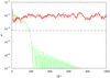 |
Fig. 3. Behaviour of a dimensionless angular momentum flux for initial vortex of perturbations defined by Eqs. (65)–(67) shown for q = −10 and M = 1. Solid and dashed lines correspond to Rnl = 1400 and Rnl = 1200, respectively. It was checked that turbulence for Rnl = 1400 does not decay at least during the three thousands shear times |q|t. The horizontal dot-dashed line corresponds to the value of αν in this case. |
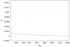 |
Fig. 4. Time-averaged angular momentum flux as function of Reynolds number for q = −10 and M = 1. Dot-dashed line corresponds to value of αν in this case. The initial vortex of perturbations is determined by Eqs. (65)–(67). |
6.3. Initial conditions
At first, we check whether the subcritical transition to turbulence we observe in our numerical experiment is in accordance with the results of LL05. Performing simulations in a cubic box, they found RT = 1200 at q = −10 for our definition of Rnl (LL05 measure time in units of the inversed shear rate, which makes their Reynolds number Rnl multiplied by q).
Generally, this is a feature of the subcritical turbulisation that RT depends on the shape and amplitude of the initial perturbations. For example, this was shown experimentally by Darbyshire & Mullin (1995) and later numerically by Faisst & Eckhardt (2004) for pipe flow. One may assume that for any particular values of q and M there are optimal initial perturbations, which provide the lowest possible value of RT. These optimals can be found by a variational approach to the non-linear Cauchy problem (see Cherubini et al. 2010 and Pringle & Kerswell 2010 for such an example). Unfortunately, this method is not easy to implement and it is time consuming. In this work we restrict a comparison with LL05 to a single variant of initial perturbations. Also, we specify the same resolution as LL05, Nx = Ny = Nz = N ≡ 64 using the cubic box.
We choose an initial condition in the form of the vortex
 (65)
(65)
 (66)
(66)
 (67)
(67)
where Ky and Kz are shearwise and spanwise dimensional wavenumbers of vortex, and the dimensionless constant A specifies the initial specific kinetic energy of perturbations, which equals A2/2.
It was revealed that for lz = 1, A = 1, and Ky = Kz = 2π the initial vortex (65)–(67) leads to self-sustained turbulence at Rturb = 1400 and damps at Rdamp = 1200 (see Figs. 3 and 4. Thus, RT = 1300, which is close to the value obtained by LL05. We additionally checked that both the decrease and the increase of the amplitude of initial vortex, respectively, up to A = 0.5 and A = 2 lead to the increase of the transition Reynolds number, respectively, up to RT = 2600 and to RT = 1500. Until the end of this section, we use the initial perturbations in the form (65)–(67) with A = 1, Ky = 2π, and Kz = 2π/lz.
6.4. Results
The picture of the subcritical transition to turbulence we extract from our simulations is presented in Table 1. For the first time (with regards to the model of unbounded uniform hydrodynamical flow considered here), we use not only the cubic box, but also a tall box with the box ratio lz > 1. The box acts as a filter with respect to perturbations of different wavelengths. It prevents the existence of both small-scale perturbations with a characteristic scale comparable and less than the size of a numerical grid-cell, and large-scale perturbations with a characteristic scale larger than the size of the box in any direction. The tall box allows perturbation harmonics with Kz/Ky = lz−1 < 1 to take part in the non-linear evolution of the perturbed flow and, probably, in the subcritical transition to turbulence. In particular, this applies to shearing spirals that effectively generate the cross-rolls. Indeed, employing Eq. (40) one estimates Kz/Ky < kz max/ϵ1/2 ≈ 0.8 for q = −10 and RT = 1300. This ratio becomes smaller as one shifts to a smaller shear rate and higher Reynolds number. For example, at q = −6.67 and RT = 104, which is the smallest shear rate examined by LL05 for the subcritical transition, its value is less than approximately 0.5. At the same time, the small size of the grid-cell is always required in order for the tightly wound spirals exhibiting large transient growth and generating high-amplitude cross-rolls to be involved into simulations.
Summary of the numerical simulations for M = 1, N = 128.
The subcritical transition in the cubic box has been observed up to q = −4 (see Table 1 and Fig. 6). This is a higher value compared to q = −6.67 reached by LL05, which is due to a higher numerical resolution used in our simulations. Indeed, assuming that turbulisation, at least indirectly, is provided by the transient growth of shearing spirals and that the smallest shearwise scalelength of perturbations resolved in the numerical scheme comprises four grid-cells, one can estimate the largest achievable Rnl provided that the shearing spirals subject to the largest swing amplification are resolved by the numerical scheme. The latter is done by Eq. (36),
 (68)
(68)
For N = 128 and q = −4 Eq. (68) yields Rnl ≈ 330 000. This is close to the RT obtained for q = −4 (see Table 1), which naturally explains why we did not see the subcritical transition at smaller |q|.
However, once we fix q = −4 and perform a set of simulations in the tall box, we find that RT falls by a factor of ∼20 as lz increases from 1.0 up to 1.5 ÷ 2 (see Fig. 5). We check that for lz > 2.0, RT tends to horizontal asymptote. Further, we managed to find the subcritical transition at even higher q = −3 in the box with the same resolution N = 128 but with the box ratio lz = 2. We regard this result as evidence for the crucial role of harmonics of perturbations with certain 0 < (Kz/Ky)T < 17. It is plausible that RT(lz) acquires an asymptotic value as soon as lz−1 ≤ (Kz/Ky)T. Such a harmonics already exists in the cubic box, however, it corresponds to n > 1 (see Eq. (59)), and, consequently, to the effective R smaller by a factor of n2 (see Eq. (60). Harmonics of a columnar shape corresponding to the highest effective R (i.e. to the largest shearwise wavelength equal to Ly), which implies the highest transient growth, emerges in the tall box only.
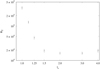 |
Fig. 5. Transition Reynolds number RT versus the box ratio lz plotted for M = 1 and q = −4. |
The question arises, what can additionally testify in favour of cross-rolls as moderators of subcritical transition? Trying to address this issue, we obtain RT in the tall box with lz = 2.0 for various q (see Table 1 and Fig. 6). It was additionally checked that the box ratio lz sufficient for RT(lz) to approach the horizontal asymptote becomes smaller as one goes to higher |q|. This guarantees that subcritical transition observed in the tall box with lz = 2.0 occurred in the presence of harmonics with (Kz/Ky)T in the range of the shear rate from q = −15 up to q = −3 covered by simulations. It was revealed that the difference between RT obtained in cubic and tall boxes increases as |q| becomes smaller. The tall box result RT = 16 250 at q = −4 allows us to evaluate the maximum growth factor of cross-rolls according to the procedure (i) formulated in Sect. 5,
 (69)
(69)
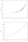 |
Fig. 6. Transition Reynolds number RT versus shear rate q in the cyclonic regime. Top panel: (1) squares represent DNS by LL05, see their Fig. 4; (2) triangles represent DNS performed in this work employing a cubic box; (3) circles represent DNS performed in this work employing a tall box with box ratio lz = 2; (4) the solid curve shows Rnl(q) corresponding to constant maximum growth factor of the cross-rolls given by equation (69) and obtained using the procedure (i) introduced in Sect. 5; (5) the dashed curve shows the same as described in (4), but with gz max/ϵ obtained using the procedure (ii) introduced in Sect. 5; bottom panel: error bars for tall box DNS represented by circles on top panel are plotted in the range q = −10 ÷ −3 according to the values of Rdamp and Rturb given in Table 1. The corresponding solid and dashed lines represent the same as on top panel but for gz max/ϵ evaluated for RT(q = −4)=15 000 (lower lines) and for RT(q = −4)=17 500 (upper lines). |
Previous inspection of the maximum optimal growth factor, Gmax, corresponding to transition to turbulence at RΩ = 0 and RΩ = −1 in the framework of the shearing sheet model (see e.g. Mukhopadhyay et al. 2005) has shown that Gmax ∼ 150 in those cases, which coincides with Eq. (69) up to the smallness factor. Using procedure (i) further in order to look for the root of Eq. (39), we obtain the curve of constant (69) on the plane (RT, q) (see the solid line in Fig. 6). Additionally, the dashed line in Fig. 6 represents the corresponding approximate Rnl(q) obtained according to procedure (ii) formulated in Sect. 5. A notable accordance is found between the growth of cross-rolls and the subcritical transition: namely, the largest growth factor of cross-rolls, as estimated in the main order in small kz, remains almost constant along the transitional path, RT(q), deduced from our non-linear stability analysis. Below we will refer to Eq. (69) as the threshold value of gz max/ϵ. If there is a common non-linear mechanism sustaining the subcritical turbulence in the uniform unbounded rotating shear flow of the cyclonic type, then it is natural to assume that it is triggered at the threshold value of the transient growth factor of relevant perturbations, at most weakly changing with the shear rate. Here we find such evidence in favour of the cross-rolls and their maximum growth factor, gz max, derived in the limit of small kz. It can be suggested that the subcritical transition, which occurs at asymptotic value of RT(lz) in the tall box simulations, takes place due to a positive non-linear feedback from the harmonics of cross-rolls with kz ≃ (Kz/Ky)T. However, the ability of cross-rolls with gz ≳ gz max to generate secondary shearing spirals subject to swing amplification sufficient to sustain turbulence remains to be shown.
We note that as q ≲ −5, the approximate analytical curve in Fig. 6 is no longer in accordance with the curve obtained accurately. The reason for that is shown in Fig. 7, where kx max, k̃x max, and  along the corresponding curves of Rnl(q) are plotted. Clearly, the limit of tightly wound spiral, |kx max|, |k̃x max| ≫ 1, is valid as far as |q|∼1 and breaks when q ≲ −5. For |q|≫1 Rnl(q) corresponding to constant (69) becomes so small that spirals are no longer tightly wound (see Eqs. (36) and (37)). At the same time, we find that the first point of the subcritical transition obtained by LL05 in the presence of rotation, RΩ > 0, which corresponds to q ≈ −33, is also in reasonable accordance with the threshold value (69). Along with the comparison of rolls and cross-rolls growth factors with each other at |q|≫1 (see the end of Sect. 5.1), this argues in favour of the assumption that, at least, when q ≳ −35, SSP is already replaced by a different self-sustaining solution incorporating the growth of cross-rolls.
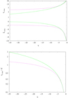 |
Fig. 7. Top panel, solid lines: roots of the set of Eqs. (34)–(35) along Rnl(q) plotted on the top panel in Fig. 6 by the solid line; dashed lines: Eqs. (36) and (37) along Rnl(q) plotted on the top panel in Fig. 6 by the dashed line. Bottom panel, solid line: |

The dependence kz max(q) obtained along the cross-rolls threshold growth factor (69) (see Fig. 7) confirms that the latter is exhibited by shearing spirals with large spanwise length scale. As long as |q| becomes smaller, the destructive role of the Coriolis force in the evolution of SFH with non-zero kz increases as compared to the pressure gradients enabling their swing amplification. That is why kz max decreases as one approaches the line of rigid rotation, which is seen in Fig. 7 (see also Eq. (40)). In turn, this naturally explains why the difference between RT obtained in cubic and tall boxes increases for smaller |q|: SFH with n = 1 (see Eq. (59)), corresponding to the growth factor (69) is progressively suppressed by periodic boundary conditions imposed in the cubic box in the spanwise direction. We note that SFH that generate the cross-rolls of the largest amplitude will be highly columnar at |q| ≈1, as far as  is estimated to become less than 0.1. If subcritical turbulence in the cyclonic regime is sustained by the non-linear feedback from the cross-rolls, it is worth checking its existence at |q|∼1 via the DNS in a very tall box.
7. Transition to turbulence: Towards the Keplerian shear across the solid-body line
Let us suppose that cross-rolls are responsible for the subcritical transition in the whole range of centrifugally stable rotating shear flows. If so, one can assume that the corresponding threshold value of the cross-rolls largest growth factor, gz max, found in the cyclonic regime (see the previous section) remains independent of the shear rate further in the quasi-Keplerian regime. Thus, we suppose that equality (69) holds for Rnl = RT across the solid body line q = 0 up to the Rayleigh line q = 2. Since the shearing spirals, which produce the threshold growth factor, become increasingly wound up as one goes from q = −∞ to q = 2 (see the bottom panel in Fig. 1 and the top panel in Fig. 7), it is sufficient to use an approximate evaluation of gz max provided by the procedure (ii) described in Sect. 5. So Rnl(q) corresponding to a constant threshold growth factor (69) extends to the quasi-Keplerian regime as shown by the curve in Fig. 8. This curve may be considered as the prediction of the subcritical transition to turbulence in homogeneous boundless quasi-Keplerian flow. Generally, the turbulence provided by the non-linear feedback from the cross-rolls is expected to occur at much higher Reynolds number ∼107 ÷ 109 in the quasi-Keplerian regime when compared to the cyclonic regime. On the one hand, this is consistent with negative results from all existing studies of the non-linear instability of the quasi-Keplerian regime, whereas on the other, even such a huge Reynolds number is feasible in astrophysical discs (see e.g. Balbus 2003). Equations (40) and (26) show that such an asymmetry of growth of the cross-rolls in the cyclonic and quasi-Keplerian regimes is controlled by the factor
which stems from the suppression of fluid vertical motion in the course of the swing amplification of SFH (see comments to Fig. 2). Consequently, we predict an asymmetry of RT(q) with respect to the line of rigid rotation: for the same absolute value of the shear rate, |q|, the subcritical transition in the quasi-Keplerian regime should occur at the substantially higher RT rather than in the cyclonic regime.
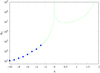 |
Fig. 8. Rnl(q) along the constant maximum growth factor of the cross-rolls given by Eq. (69), where gz max/ϵ is obtained approximately using procedure (ii) introduced in Sect. 5. The circles represent DNS performed in this work using a tall box with box ratio lz = 2 (see Sect. 6 for details). The curve is matched to the circle at q = −4, which corresponds to RT = 16 250 (see Table 1). |
Let us note that the enhanced non-linear stability of quasi-Keplerian flow follows from our DNS in the cyclonic regime together with the results of LL05 and Rincon et al. (2007) discussed in Introduction. Indeed, the curves on top panel in Fig. 6 indicate that RT ≈ 3 × 10⁵ at q = −1.5. At the same time, from extrapolation of DNS by LL05 carried out at RΩ < −1, see expressions in their Fig. 7, it is expected that RT ≳ 109 at q = 1.5. This independently shows an asymmetry of RT(q) with respect to change of sign of q. However, the swing amplification itself produces maximum growth factor  , which would yield a symmetric RT ∝ |q|−1 with respect to change from cyclonic to quasi-Keplerian shear rate.
It is noteworthy that prediction of RT in Fig. 8 combined with extrapolations of DNS suggested by LL05 for quasi-Keplerian regime gives the most stable rotating flow located at super-Keplerian shear rate q ∼ 1.7 ÷ 1.8.
Further, since in the vicinity of the solid-body line RT naturally tends to infinity (cf. Eqs. (41) and (36), (40) at |q|→0), a minimal RT is predicted for the quasi-Keplerian regime. The corresponding most “favourable” value of q can be immediately estimated in the limit of tightly wound SFH. Using Eq. (41) in combination with Eqs. (36) and (40) and the condition R ≫ 1, we find that constant gz max corresponds to

which yields minimal RT at q = 1/2. So, RT(q = 1/2) exceeds 107, while the transition at the Keplerian shear, q = 3/2, may occur at R approaching ∼108. Hence, the super-Keplerian flow 3/2 < q < 2 is predicted to be the most non-linearly stable throughout the whole range of centrifugally stable rotating shear flows. Notably, most of the efforts to detect turbulence in the quasi-Keplerian regime in laboratory experiments and DNS have been made at super-Keplerian shear rates. In contrast, our results suggest that one should extend the turbulent solutions obtained so far in the cyclonic regime to smaller |q| and then across the solid-body line, finally focusing the efforts on sub-Keplerian rotation. The effective numerical viscosity existing in DNS is approximately proportional to the distance between the nodes of the numerical grid. If so, the maximum Reynolds number accessible in DNS is ∝ N2. Then, assuming that RT ≈ 40 000 at q = −3, see Table 1, is the maximum accessible Rnl for N = 128 in tall box, we suppose that in order to be able to check hypothetical transition to hydrodynamic turbulence in quasi-Keplerian flow, at least for “favourable” q = 1/2, N ≳ 2000 is required. This is quite a high DNS resolution, however, it is not unreachable for the most powerful modern supercomputers.
8. Summary
Angular momentum transport in boundary layers around the accreting weakly magnetised stars may be produced by turbulent fluctuations. Here we suggest that subcritical turbulence in boundless and homogeneous rotating shear flow of the cyclonic type, which is a local representative of the boundary layer, is supplied with energy by nearly optimal shearing spirals that generate essentially 3D vortices of high amplitude as a “byproduct” of swing amplification. We call those 3D vortices “cross-rolls” in order to distinguish them from the known streamwise rolls generated via the anti-lift-up mechanism in a flow on the Rayleigh line. Such turbulence must be sustained by a novel type of positive non-linear feedback from the cross-rolls, which would recover the basin of growing shearing spirals. Furthermore, we suppose that this scenario also works in the quasi-Keplerian regime. These suggestions are supported by the following evidence.
-
i)
As well as known spanwise invariant (columnar) shearing spirals, shearing spirals with small but non-zero spanwise wavenumber are subject to swing amplification, which causes their transient growth almost up to the highest possible values corresponding to a growth factor much greater that unity. Thus, these vortices satisfy a necessary condition for the subcritical transition in both the cyclonic and quasi-Keplerian regimes. At the same time, it is known that all shearing harmonics with kz ≳ 1 do not exhibit considerable transient growth since they drastically degenerate into epicyclic oscillations.
-
ii)
The substantial decrease of RT and the existence of an asymptotic value of RT(lz) for large lz found in the tall box simulations (see Fig. 5) indicates that these perturbations are crucial for the transition and sustenance of subcritical turbulence, at least in the cyclonic regime. This is the most striking evidence that the cross-rolls could be ingredients of positive non-linear feedback completing the bypass scenario in centrifugally stable rotating shear flows.
-
iii)
It is revealed that the maximum growth factor of cross-rolls decreases as the shear rate alters from q = −∞ through the solid-body line q = 0 up to q = 2 (see Fig. 1). Moreover, its constant value accords with the curve of RT(q < 0) obtained in tall box simulations (see Fig. 6). We regard this value as the threshold growth factor, which triggers the non-linear sustenance of subcritical turbulence in the cyclonic regime. On the contrary, the spanwise invariant shearing spirals with kz = 0 do not produce any 3D vortices and acquire a growth factor symmetric with respect to change between the cyclonic and quasi-Keplerian regimes at the same |q|. However, DNS of turbulence in the cyclonic regime performed by LL05 and in this work far beyond the zone of the lift-up effect show a strong variation of the 2D growth factor along the obtained RT(q < 0).
-
iv)
The disappearance of the cross-rolls in the vicinity of q = 2 naturally explains the asymmetry of the transition to turbulence revealed in DNS close to RΩ = −1 versus RΩ = 0: the bypass scenario based on the transient growth of shearing spirals with small but non-zero kz for q < 0 replaces SSP, retaining the non-linear instability of the cyclonic flow immediately after the lift-up ceases to operate, whereas a similar situation with the anti-lift-up mechanism is not realised in the case of quasi-Keplerian rotation.
-
v)
The cross-rolls are the only high-amplitude essentially 3D vortices that can be generated via the transient growth mechanism in the whole range of centrifugally stable shear rates, provided that the Reynolds number is sufficiently high. They create the vorticity (namely, its shearwise and streamwise components), which must be of crucial importance for 3D turbulence.
-
vi)
The transition to turbulence in the tall box is observed until smaller |q| than that in the cubic box at the same numerical resolution is obtained (see. Fig. 6). Generally, a sensitivity of the transition to the shape of a box indicates the anisotropic nature of subcritical turbulence. In future work, the properties of subcritical turbulence including details of the non-linear sustaining process, as well as the precise role of the cross-rolls in it, should be studied employing, in particular, 3D Fourier analysis in k-space (see Mamatsashvili et al. (2016) and Gogichaishvili et al. (2017) for an examples of such studies in application to non-rotating shear flow and Keplerian flow with an azimuthal magnetic field).
-
i)
The dynamics of perturbations in the plane orthogonal to the spanwise direction remain approximately the same as for spanwise invariant (columnar) shearing spirals, which is the 2D swing amplification process.
-
ii)
Spanwise acceleration of fluid elements is determined by the swing amplification.
-
iii)
Spanwise velocity perturbation increases while the shearing spiral swings from trailing to leading in the cyclonic flow and vice versa in the quasi-Keplerian flow. After that, the spiral is wound by the shear, which causes the decay of streamwise and shearwise velocity perturbations, whereas the spanwise velocity perturbation tends to an asymptotic inviscid non-zero value proportional to the net impulse given to fluid elements in spanwise direction. The latter depends on the shear rate and vanishes as q → 2. Viscous damping results in a maximum value of the initial winding of shearing spiral and additionally in the maximum of spanwise velocity, which appears after the instant of swing (see Eqs. (36) and (37) giving the locations of those extrema in the limit of tightly wound spirals).
-
iv)
Assuming that the cross-rolls of the largest amplitude sustain turbulence throughout the range of centrifugally stable rotating shear flows and the threshold value of their growth factor found in the cyclonic regime (see Eq. (69)) remains the same, we obtain a tentative prediction of RT(q) for the quasi-Keplerian regime, where hydrodynamical turbulence is not yet discovered. In particular, we find that the lowest RT ∼ 107 in the quasi-Keplerian regime must be attained at a sub-Keplerian shear rate q ≈ 1/2.
-
v)
The threshold value of the cross-rolls growth factor (69) exceeds the maximum growth factors of streaks and rolls generated via lift-up and anti-lift-up up to the shear rates, very close, respectively, to non-rotating flow and to flow on the Rayleigh line (see Sect. 5.1).
The cross-rolls’ appearance is shown in the top panels in Fig. 9 (see also Appendix A for the explanation of this representation). The growth factor of the corresponding shearing spiral is plotted by a solid curve in Fig. 1. For comparison, the rolls generated from axisymmetric streaks via anti-lift-up with the same kx and kz but in the flow close to the Rayleigh line are shown on the bottom panels in Fig. 9. The former and the latter ones are aligned in the shearwise and the streamwise directions, respectively. Furthermore, in contrast to rolls, the cross-rolls are essentially 3D vortices, since they are of a finite length along their axes of rotation, being contracted by the background shear ∝ |k̃x|−1. In combination with the opposite rotation of the adjacent cross-rolls, this causes monotonic growth of ωy ∝ |k̃x| in areas between the adjacent cross-rolls, in the vicinity of for example point (x = λx/4, y = 0, z = λz/4). As one can see, the cross-rolls coexist with “planar” eddies fading after the instant of swing. Such a complicated structure of the perturbation velocity field requires a new concept of non-linear feedback, which may be completely different from both SSP and a scheme associated with streamwise rolls in the flow on the Rayleigh line. The latter itself remains unknown.
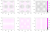 |
Fig. 9. Left, middle, and right panels: cross-sections of shearing spiral velocity pattern, respectively, in (y, z)-, (x, z)-, and (x, y)-planes, which contain the point x = y = z = 0. The colour represents the velocity absolute value normalised by its maximum value separately for the top and bottom panels. Top panels: kx = −141, kz = 0.1, k̃x = 43, and q = 1.5. The wavelengths are λx = 2π/k̃x, λy = 2π, λz = 2π/kz. Bottom panels: kx = −141, kz = 0.1, and t = π/(2σ), where σ is defined in Sect. 5.1; the shear rate is q = 1.99. The wavelengths are λx = 2π/kx, λy = ∞, λz = 2π/kz. The extraction of the shearing spiral velocity pattern is described in detail in Appendix A. |
The prediction of RT(q) obtained in this work (see Fig. 8) makes it clear that, at least for boundless homogeneous flows, the issue of the transition to turbulence in the Keplerian regime should be attacked from the side of the cyclonic regime. This implies the crossing of the solid-body line, RΩ = +∞ →RΩ = −∞, which is not evident while looking at the axis of RΩ. However, we suppose that RT ∼ 107 at the most “favourable” sub-Keplerian shear rate q ∼ 1/2, which presumably requires a resolution of N ≳ 2000 for the spectral Fourier code to be able to test the non-linear instability of the quasi-Keplerian regime. Still, such an extraordinary non-linear stability of Keplerian flow may be defeated by the huge spatial scales of real astrophysical discs, leading to R = 1010 ÷ 1013.
Actually, these are the radially averaged shear rates.
In hydrodynamical literature it is also called the Orr mechanism.
Especially, bearing in mind a result of Meseguer (2002) who revealed that subcritical transition observed in counter-rotating flow between the cylinders occurs along the line of constant Gmax on the plane of the Reynolds numbers corresponding to inner and outer cylinders (see Fig. 2 therein).
A rigorous restriction on the value of kz including the possible smallness of q will be made after we have the corresponding modified solution at hand (see Sect. 3.3).
Cf. Eq. (40) below.
Acknowledgments
We kindly thank Professor K. Postnov and Professor P. Ivanov for genuine interest in the subject of this study and for a number of discussions during the preparation of the manuscript. The research is carried out using the equipment of the shared research facilities of HPC computing resources at Lomonosov Moscow State University (see paper Sadovnichy et al. 2013 for its detailed description). Equipment for the reported study was granted in part by the M. V. Lomonosov Moscow State University Programme of Development. DNR was supported by grant RSF 14-12-00146 when writing Sect. 6 of this paper. VVZ was supported in part by RFBR grant 15-02-08476 and by programme 7 of the Presidium of Russian Academy of Sciences.
References
- Abramowicz, M. A., Czerny, B., Lasota, J. P., & Szuszkiewicz, E. 1988, ApJ, 332, 646 [NASA ADS] [CrossRef] [Google Scholar]
- Afshordi, N., Mukhopadhyay, B., & Narayan, R. 2005, ApJ, 629, 373 [NASA ADS] [CrossRef] [Google Scholar]
- Baggett, J. S., & Trefethen, L. N. 1997, Phys. Fluids, 9, 1043 [NASA ADS] [CrossRef] [MathSciNet] [Google Scholar]
- Balbus, S. A. 2003, ARA&A, 41, 555 [NASA ADS] [CrossRef] [Google Scholar]
- Balbus, S. A., & Hawley, J. F. 2006, ApJ, 652, 1020 [NASA ADS] [CrossRef] [Google Scholar]
- Belyaev, M. A., Rafikov, R. R., & Stone, J. M. 2013, ApJ, 770, 67 [NASA ADS] [CrossRef] [Google Scholar]
- Bisnovatyi-Kogan, G. S. 1994, MNRAS, 269, 557 [NASA ADS] [CrossRef] [Google Scholar]
- Burin, M. J., & Czarnocki, C. J. 2012, J. Fluid Mech., 709, 106 [NASA ADS] [CrossRef] [Google Scholar]
- Butler, K. M., & Farrell, B. F. 1992, Phys. Fluids A, 4, 1637 [NASA ADS] [CrossRef] [Google Scholar]
- Chagelishvili, G. D., Zahn, J.-P., Tevzadze, A. G., & Lominadze, J. G. 2003, A&A, 402, 401 [NASA ADS] [CrossRef] [EDP Sciences] [Google Scholar]
- Chagelishvili, G., Hau, J.-N., Khujadze, G., & Oberlack, M. 2016, Phys. Rev. Fluids, 1, 043603 [NASA ADS] [CrossRef] [Google Scholar]
- Cherubini, S., de Palma, P., Robinet, J.-C., & Bottaro, A. 2010, Phys. Rev. E, 82, 066302 [NASA ADS] [CrossRef] [Google Scholar]
- Darbyshire, A. G., & Mullin, T. 1995, J. Fluid Mech., 289, 83 [NASA ADS] [CrossRef] [Google Scholar]
- Edlund, E. M., & Ji, H. 2014, Phys. Rev. Lett., 89, 021004 [NASA ADS] [Google Scholar]
- Ellingsen, T., & Palm, E. 1975, Phys. Fluids, 18, 487 [NASA ADS] [CrossRef] [Google Scholar]
- Faisst, H., & Eckhardt, B. 2004, J. Fluid Mech., 504, 343 [NASA ADS] [CrossRef] [Google Scholar]
- Gogichaishvili, D., Mamatsashvili, G., Horton, W., Chagelishvili, G., & Bodo, G. 2017, ApJ, 845, 70 [NASA ADS] [CrossRef] [Google Scholar]
- Grossmann, S. 2000, Rev. Mod. Phys., 72, 603 [NASA ADS] [CrossRef] [Google Scholar]
- Grossmann, S., Lohse, D., & Sun, C. 2016, Ann. Rev. Fluid Mech., 48, 150724171740009 [Google Scholar]
- Hamilton, J. M., Kim, J., & Waleffe, F. 1995, J. Fluid Mech., 287, 317 [NASA ADS] [CrossRef] [Google Scholar]
- Hawley, J. F., Gammie, C. F., & Balbus, S. A. 1995, ApJ, 440, 742 [NASA ADS] [CrossRef] [Google Scholar]
- Hawley, J. F., Balbus, S. A., & Winters, W. F. 1999, ApJ, 518, 394 [NASA ADS] [CrossRef] [Google Scholar]
- Henningson, D. 1996, Phys. Fluids, 8, 2257 [NASA ADS] [CrossRef] [Google Scholar]
- Horton, W., Kim, J.-H., Chagelishvili, G. D., Bowman, J. C., & Lominadze, J. G. 2010, Phys. Rev. E, 81, 066304 [NASA ADS] [CrossRef] [Google Scholar]
- Inogamov, N. A., & Sunyaev, R. A. 1999, Astron. Lett., 25, 269 [NASA ADS] [Google Scholar]
- Ioannou, P. J., & Kakouris, A. 2001, ApJ, 550, 931 [NASA ADS] [CrossRef] [Google Scholar]
- Johnson, B. M., & Gammie, C. F. 2005, ApJ, 635, 149 [NASA ADS] [CrossRef] [Google Scholar]
- Lesur, G., & Longaretti, P.-Y. 2005, A&A, 444, 25 [NASA ADS] [CrossRef] [EDP Sciences] [Google Scholar]
- Lithwick, Y. 2007, ApJ, 670, 789 [NASA ADS] [CrossRef] [Google Scholar]
- Lithwick, Y. 2009, ApJ, 693, 85 [NASA ADS] [CrossRef] [Google Scholar]
- Mamatsashvili, G., Khujadze, G., Chagelishvili, G., et al. 2016, Phys. Rev. E, 94, 023111 [Google Scholar]
- Maretzke, S., Hof, B., & Avila, M. 2014, J. Fluid Mech., 742, 254 [NASA ADS] [CrossRef] [Google Scholar]
- Meseguer, Á. 2002, Phys. Fluids, 14, 1655 [NASA ADS] [CrossRef] [Google Scholar]
- Mukhopadhyay, B., Afshordi, N., & Narayan, R. 2005, ApJ, 629, 383 [NASA ADS] [CrossRef] [Google Scholar]
- Mukhopadhyay, B., Afshordi, N., & Narayan, R. 2006, Adv. Space Res., 38, 2877 [NASA ADS] [CrossRef] [Google Scholar]
- Narayan, R., & Popham, R. 1993, Nature, 362, 820 [NASA ADS] [CrossRef] [Google Scholar]
- Ostilla-Mónico, R., Verzicco, R., Grossmann, S., & Lohse, D. 2014, J. Fluid Mech., 748, R3 [CrossRef] [Google Scholar]
- Ostilla-Mónico, R., Verzicco, R., & Lohse, D. 2016, J. Fluid Mech., 799, R1 [CrossRef] [Google Scholar]
- Philippov, A. A., Rafikov, R. R., & Stone, J. M. 2016, ApJ, 817, 62 [NASA ADS] [CrossRef] [Google Scholar]
- Popham, R., & Sunyaev, R. 2001, ApJ, 547, 355 [NASA ADS] [CrossRef] [Google Scholar]
- Popham, R., Narayan, R., Hartmann, L., & Kenyon, S. 1993, ApJ, 415, L127 [NASA ADS] [CrossRef] [Google Scholar]
- Pringle, C. C. T., & Kerswell, R. R. 2010, Phys. Rev. Lett., 105, 154502 [NASA ADS] [CrossRef] [Google Scholar]
- Razdoburdin, D. N., & Zhuravlev, V. V. 2015, Phys. Usp., 58, 1031 [NASA ADS] [CrossRef] [Google Scholar]
- Razdoburdin, D. N., & Zhuravlev, V. V. 2017, MNRAS, 467, 849 [NASA ADS] [CrossRef] [Google Scholar]
- Reddy, S. C., & Henningson, D. S. 1993, J. Fluid Mech., 252, 209 [NASA ADS] [CrossRef] [Google Scholar]
- Rincon, F., Ogilvie, G. I., & Cossu, C. 2007, A&A, 463, 817 [NASA ADS] [CrossRef] [EDP Sciences] [Google Scholar]
- Rincon, F., Ogilvie, G. I., Proctor, M. R. E., & Cossu, C. 2008, Astron. Nachr., 329, 750 [NASA ADS] [CrossRef] [Google Scholar]
- Sadovnichy, V., Tikhonravov, A., Voevodin, V., & Opanasenko, V. 2013, Contemporary High Performance Computing: From Petascale toward Exascale , (Boca Raton, USA: Chapman & Hall/CRC Computational Science), 283 [Google Scholar]
- Schartman, E., Ji, H., Burin, M. J., & Goodman, J. 2012, A&A, 543, A13 [NASA ADS] [CrossRef] [EDP Sciences] [Google Scholar]
- Shakura, N. I., & Sunyaev, R. A. 1973, A&A, 24, 337 [NASA ADS] [Google Scholar]
- Shakura, N. I., & Sunyaev, R. A. 1988, Adv. Space Res., 8, 135 [NASA ADS] [CrossRef] [Google Scholar]
- Shen, Y., Stone, J. M., & Gardiner, T. A. 2006, ApJ, 653, 513 [NASA ADS] [CrossRef] [Google Scholar]
- Shi, L., Hof, B., Rampp, M., & Avila, M. 2017, Phys. Fluids, 29, 044107 [NASA ADS] [CrossRef] [Google Scholar]
- Stone, J. M., & Gardiner, T. A. 2010, ApJS, 189, 142 [NASA ADS] [CrossRef] [Google Scholar]
- Stone, J. M., Gardiner, T. A., Teuben, P., Hawley, J. F., & Simon, J. B. 2008, ApJS, 178, 137 [NASA ADS] [CrossRef] [Google Scholar]
- Trefethen, L. N., Trefethen, A. E., Reddy, S. C., & Driscoll, T. A. 1993, Science, 261, 578 [NASA ADS] [CrossRef] [MathSciNet] [PubMed] [Google Scholar]
- Umurhan, O. M., & Regev, O. 2004, ApJ, 427, 855 [NASA ADS] [Google Scholar]
- Waleffe, F. 1997, Phys. Fluids, 9, 883 [NASA ADS] [CrossRef] [Google Scholar]
- Yecko, P. A. 2004, A&A, 425, 385 [NASA ADS] [CrossRef] [EDP Sciences] [Google Scholar]
- Zhuravlev, V. V., & Razdoburdin, D. N. 2014, MNRAS, 442, 870 [NASA ADS] [CrossRef] [Google Scholar]
Appendix A: Representation of cross-rolls
In order to plot the velocity perturbation in Fig. 9, we take the imaginary part of SFH given by Eq. (5), where the Fourier amplitudes of the velocity perturbations, ûx,y,z, are given by the analytic solution (17,18, 25). Explicitly, we have
![Mathematical equation: $$ \begin{aligned} \mathfrak{I} \left[ \begin{array}{c} u_x\\ u_y\\ u_z \end{array} \right]= \left( \begin{array}{c} \hat{u}_x\\ \hat{u}_y\\ \hat{u}_z \end{array} \right) \sin (\tilde{k}_x x+y+k_z z)= \mathbf{C}_1 + \mathbf{C}_2 + \mathbf{C}_3 + \mathbf{C}_4, \end{aligned} $$](/articles/aa/full_html/2018/11/aa33024-18/aa33024-18-eq97.gif) (A.1.)
(A.1.)
where
Therefore, SFH is nothing but a combination of the single velocity pattern, C1, with its duplicates translated along the coordinate axes on one-fourth of the corresponding wavelength. This velocity pattern has the form
 (A.2.)
and is represented in Fig. 9 by the three mutually perpendicular cross-sections having the common point {x = 0, y = 0, z = 0}.
Appendix B: Effect of finite numerical resolution
In order to reveal the influence of the numerical viscosity on the transition to turbulence at terminally high Rnl, we fix q = −4 and perform a set of additional simulations with exactly the same setup as described in Sect. 6. The results are shown in table B.1.
Summary of additional numerical simulations for M = 1 and q = −4.
The value of RT obtained in cubic box substantially drops as we increase resolution up to N = 192. This is to be expected, since at N = 128 RT is close to the restriction (68). However, an even higher resolution, N = 256, does not lead to further decrease of RT: we conclude that convergence is achieved in this case. At the same time, RT in tall box is only weakly affected by the increase of resolution. Thus, there is a difference between the transition Reynolds numbers in cubic and tall boxes, which cannot be attributed to effect of finite resolution.
All Tables
All Figures
|
Fig. 1. Short-dashed, dotted, long-dashed, solid, and dot-dashed curves: gz(k̃x) (top panel) and g(k̃x) (bottom panel) for transient growth of the particular SFH at q = −5, −1.5, 0.5, 1.5, and 1.6, respectively. In each case, kx and kz are chosen in such a way that SFH attains the constant value gz(k̃x max) = gz max ≈ 180ϵ (see Sect. 3.3 for definition of ϵ). This value of gz max/ϵ is obtained employing the procedure (ii) (see this section) in order to fit the transitional dependence RT(q) found in the tall box simulations of turbulence in the cyclonic regime (see Sect. 6) for details and the dashed curve on the top panel in Figs. 6 and 8. Solid and dashed horizontal lines on the bottom panel mark the value of corresponding gz max for ϵ = 1 and ϵ = 0.1, respectively. |
| In the text | |
|
Fig. 2. Short-dashed, dotted, long-dashed, and solid curves: ℑ[Ŵ](k̃x) according to Eq. (19) for q = −5, −1.5, 0.5, and 1.5, respectively. The growth factors of the corresponding SFHs are shown in Fig. 1. There is no curve for q = 1.6 since it virtually coincides with the curve for q = 1.5. |
| In the text | |
|
Fig. 3. Behaviour of a dimensionless angular momentum flux for initial vortex of perturbations defined by Eqs. (65)–(67) shown for q = −10 and M = 1. Solid and dashed lines correspond to Rnl = 1400 and Rnl = 1200, respectively. It was checked that turbulence for Rnl = 1400 does not decay at least during the three thousands shear times |q|t. The horizontal dot-dashed line corresponds to the value of αν in this case. |
| In the text | |
|
Fig. 4. Time-averaged angular momentum flux as function of Reynolds number for q = −10 and M = 1. Dot-dashed line corresponds to value of αν in this case. The initial vortex of perturbations is determined by Eqs. (65)–(67). |
| In the text | |
|
Fig. 5. Transition Reynolds number RT versus the box ratio lz plotted for M = 1 and q = −4. |
| In the text | |
|
Fig. 6. Transition Reynolds number RT versus shear rate q in the cyclonic regime. Top panel: (1) squares represent DNS by LL05, see their Fig. 4; (2) triangles represent DNS performed in this work employing a cubic box; (3) circles represent DNS performed in this work employing a tall box with box ratio lz = 2; (4) the solid curve shows Rnl(q) corresponding to constant maximum growth factor of the cross-rolls given by equation (69) and obtained using the procedure (i) introduced in Sect. 5; (5) the dashed curve shows the same as described in (4), but with gz max/ϵ obtained using the procedure (ii) introduced in Sect. 5; bottom panel: error bars for tall box DNS represented by circles on top panel are plotted in the range q = −10 ÷ −3 according to the values of Rdamp and Rturb given in Table 1. The corresponding solid and dashed lines represent the same as on top panel but for gz max/ϵ evaluated for RT(q = −4)=15 000 (lower lines) and for RT(q = −4)=17 500 (upper lines). |
| In the text | |
|
Fig. 7. Top panel, solid lines: roots of the set of Eqs. (34)–(35) along Rnl(q) plotted on the top panel in Fig. 6 by the solid line; dashed lines: Eqs. (36) and (37) along Rnl(q) plotted on the top panel in Fig. 6 by the dashed line. Bottom panel, solid line: |
| In the text | |
|
Fig. 8. Rnl(q) along the constant maximum growth factor of the cross-rolls given by Eq. (69), where gz max/ϵ is obtained approximately using procedure (ii) introduced in Sect. 5. The circles represent DNS performed in this work using a tall box with box ratio lz = 2 (see Sect. 6 for details). The curve is matched to the circle at q = −4, which corresponds to RT = 16 250 (see Table 1). |
| In the text | |
|
Fig. 9. Left, middle, and right panels: cross-sections of shearing spiral velocity pattern, respectively, in (y, z)-, (x, z)-, and (x, y)-planes, which contain the point x = y = z = 0. The colour represents the velocity absolute value normalised by its maximum value separately for the top and bottom panels. Top panels: kx = −141, kz = 0.1, k̃x = 43, and q = 1.5. The wavelengths are λx = 2π/k̃x, λy = 2π, λz = 2π/kz. Bottom panels: kx = −141, kz = 0.1, and t = π/(2σ), where σ is defined in Sect. 5.1; the shear rate is q = 1.99. The wavelengths are λx = 2π/kx, λy = ∞, λz = 2π/kz. The extraction of the shearing spiral velocity pattern is described in detail in Appendix A. |
| In the text | |
Current usage metrics show cumulative count of Article Views (full-text article views including HTML views, PDF and ePub downloads, according to the available data) and Abstracts Views on Vision4Press platform.
Data correspond to usage on the plateform after 2015. The current usage metrics is available 48-96 hours after online publication and is updated daily on week days.
Initial download of the metrics may take a while.