| Issue |
A&A
Volume 619, November 2018
|
|
|---|---|---|
| Article Number | A22 | |
| Number of page(s) | 13 | |
| Section | Stellar atmospheres | |
| DOI | https://doi.org/10.1051/0004-6361/201833016 | |
| Published online | 01 November 2018 | |
Using machine learning algorithms to measure stellar magnetic fields⋆
1
Instituto de Astronomía – Universidad Nacional Autónoma de México, Apdo. Postal 877, 22860 Ensenada, BC, Mexico
e-mail: jramirez@astro.unam.mx
2
Laboratorio de Cómputo Inteligente – Instituto Politécnico Nacional, Av. Juan de Dios Bátiz s/n, 07738 CDMX, Mexico
3
CUCEA, Universidad de Guadalajara, Periférico Norte 799, Los Belenes, 45100 Zapopan Jalisco, Mexico
Received:
13
March
2018
Accepted:
26
July
2018
Context. Regression methods based on machine learning algorithms (MLA) have become an important tool for data analysis in many different disciplines.
Aims. In this work, we use MLA in an astrophysical context; our goal is to measure the mean longitudinal magnetic field in stars (Heff) from polarized spectra of high resolution, through the inversion of the so-called multi-line profiles.
Methods. Using synthetic data, we tested the performance of our technique considering different noise levels: In an ideal scenario of noise-free multi-line profiles, the inversion results are excellent; however, the accuracy of the inversions diminish considerably when noise is taken into account. We therefore propose a data pre-process in order to reduce the noise impact, which consists of a denoising profile process combined with an iterative inversion methodology.
Results. Applying this data pre-process, we find a considerable improvement of the inversions results, allowing to estimate the errors associated to the measurements of stellar magnetic fields at different noise levels.
Conclusions. We have successfully applied our data analysis technique to two different stars, attaining for the first time the measurement of Heff from multi-line profiles beyond the condition of line autosimilarity assumed by other techniques.
Key words: magnetic fields / line: profiles / polarization / radiative transfer / methods: data analysis
The training data sets used here are available at www.astrosen.unam.mx/~julio/ML_mzs and at the CDS via anonymous ftp to cdsarc.u-strasbg.fr (130.79.128.5) or via http://cdsarc.u-strasbg.fr/viz-bin/qcat?J/A+A/619/A22
© ESO 2018
1. Introduction
Magnetic fields are a key ingredient in the study of the stellar evolution and yet many of their aspects are still unkown, due to the difficulty of detecting, measuring, and mapping (whenever this is possible) surface magnetic fields in stars other than the Sun, among other issues.
Nonetheless, a lot of progress has been made in recent years in the study and observation of stellar magnetic fields, and some facts are now well established. For example, non-chemically peculiar massive stars can host stable strong dipolar configurations and the mean longitudinal magnetic fields (Heff) for these stars vary from tens to thousands of Gauss (e.g. Donati & Landstreet 2009; Wade et al. 2016; Grunhut et al. 2017) and the solar type stars during the main sequence phase harbour more complex magnetic geometries and exhibit much weaker effective fields (Heff), by at least one order of magnitude, namely, in the order of tens of Gauss or less (e.g. Petit et al. 2008; Marsden et al. 2014). These two examples are of interest for this work from a data analysis point of view, because their results were obtained using the so-called multi-lines approach. This means that to retrieve a signal in the circular polarised Stokes parameter (V), in order to detect and to subsequently measure the magnetic field, it is necessary to co-add as many individual spectral lines as possible. The line addition permits to boost the signal-to-noise ratio (S/N) value in the resulting “mean” circular profile. Otherwise, the individual V profiles are in general systematically below the noise level.
The underlying idea of grouping many lines together into a single one is that the noise addition is incoherent while the addition of the V profiles is coherent (Semel & Li 1996), that is, the higher the number of individual profiles co-added, the better the S/N that is retrieved in the mean profile. Typically, an ad-hoc selection of unblended lines is performed establishing a linear relation between the mean circular profile and the mean longitudinal magnetic field. The number of lines to combine depends on the spectral type of the star and on the instrumental resolution. In the case of modern high-resolution spectropolarimeters such as HARPS, ESPaDOnS or NARVAL, the total number can reach up to ten thousand lines or more for late-type stars.
Different techniques have been proposed to perform the line addition, and they can be roughly divided into two groups: 1) those where line addition is based on the assumption that all the lines are autosimilars (e.g. Donati et al. 1997; Wade et al. 2000; Kochukhov et al. 2010) or applying a deblending process to extend the range of applicability of the technique (Sennhauser et al. 2009; Sennhauser & Berdyugina 2010) and 2) those where the line autosimilarity assumption is not necessary (e.g. Semel et al. 2006, 2009; Ramírez Vélez et al. 2010). The mean profiles obtained using approaches of the former group are called leastsquare- deconvolved (LSD) profiles after the work of Donati et al. (1997), and they require the use of unblended lines, while the mean profiles issued from the latter group are called multi-Zeeman-signatures (MZS) after the work of Semel et al. (2009), and in this case the mean profiles are established including blended and unblended lines.
For the LSD profiles, the measurement of the strength of the mean longitudinal magnetic fields can be done through the weak field approximation (WFA, see e.g. Jefferies et al. 1989), or alternatively, with the centre-of-gravity method (COG, see e.g. Rees & Semel 1979) through the first-order moment of the mean circular profile (Mathys 1989). The employment of the WFA and of the COG methods are of great utility because they allow to measure the effective magnetic field without recourse to radiative transfer calculations. Nowadays, the COG method is the first-choice technique used to determine Heff from the LSD profiles. Nevertheless, both approaches have limitations due to assumption of self-similarity of the lines, having to fulfil both conditions simultaneously: the use of unblended lines and the measurement of weak magnetic fields. The range of application in the data analysis is therefore difficult to determine precisely. For example, concerning the second condition related to the strength of the magnetic fields, Kochukhov et al. (2010) stated a maximum of 2 kG as limit for the analysis of circular polarised LSD profiles; however, as noticed by Carroll & Strassmeier (2014) the limit of the WFA of local profiles, that is, to reach the Zeeman saturation regime in individual lines, is around 1 kG for lines in the optical wavelength range. In any case, to bypass the inherent limitations associated to the use of the LSD profiles and to dispose of a more general approach, in this work we continue the development of a method based on the analysis of the MZS profiles.
In a previous work, (Ramírez Vélez et al. 2016; hereafter Paper I), we presented a new inversion code for the measurement of stellar magnetic fields using a complete radiative transfer approach. We used a solar-type star (Teff = 5500 K) as case of study to show that the MZSs can be used to correctly retrieve the stellar longitudinal magnetic field in cool stars. The proposed methodology illustrates that it is feasible to infer Heff, in the context of the multi-lines approach, beyond the assumption autosimilarity of lines, that is, beyond the employment of the COG method (or the WFA).
The inversion code used in Paper I was based on a look-up table, that is, the higher the number of stellar MZSs contained in the table, the better the results obtained. This fact makes our technique a very CPU-time consuming method. In this work, we incorporate the use of machine learning algorithms to remarkably decrease the number of synthetic stellar spectra required to properly determine Heff.
In Sect. 2, we show the performance of different machine learning algorithms for the inversion of ideal noiseless MZSs, to subsequently show that the effectivity of the regression algorithms is strongly affected when noise is included, even for very small noise levels. In Sect. 3 we incorporate pre-process data analysis to reduce the noise effect when inferring Heff. In Sect. 4 we apply our method to two real cases and compare our results to previous ones published in others studies, before finally drawing some general conclusions in Sect. 5.
2. The machine learning strategy
In the stellar physics domain, the number of published studies using analysis methods based on machine learning algorithms has been growing, especially in recent years, either for classification of stars (e.g. Richards et al. 2011; Armstrong et al. 2016), in the search of exoplanets (e.g. Davies et al. 2016), or in the determination of stellar fundamental parameters (e.g. Bellinger et al. 2016; Verma et al. 2016; Angelou et al. 2017), among many others. In this work we use the machine learning approach in the context of the study of stellar magnetic fields.
As previously mentioned, in Paper I we performed inversions of MZSs using a code based on a look-up table strategy, meaning that given a number of MZSs to invert we find, as a solution, the closest-norm MZSs in the table. The MZSs were constructed adopting the eccentric tilted dipole model (Stift 1975). In this model, we considered as free: 1) all the parameters that describe the magnetic geometry of the dipolar configuration (the three Eulerian angles α, β, γ, and the inclination angle (i) of the stellar rotation axis with respect to the line of sight), 2) the position of the magnetic dipole inside of the star given by two coordinates (X2, X3), and 3) the strength of the dipolar moment (m), leading to a total of seven free parameters. It turned out that in order to obtain good enough inversion results, we were required to calculate 7500 stellar spectra models. For each synthetic spectrum, we randomly varied the seven free parameters, covering a spectral range from 350 to 1000 nm, giving a total close to 350 000 wavelength points per spectra. This huge number of thousands of stellar spectra, required to shape the table, demands a lot of computer calculation time which damps the employment of our technique for the analysis of large databases, such as Polarbase1 (Petit et al. 2014), where hundreds of observed spectra of cool stars can be found.
To reduce the required number of stellar spectra to invert the MZSs, in this work we implemented three different regression methods based on machine learning algorithms. All three of these regression models belong to the supervised paradigm and are included in the Scikit-learn software package (Pedregosa et al. 2011) of the Python language. The employed regressions are: 1) the Bayesian Ridge Linear Regression (BR), 2) the Support Vector Machine (SVM), and 3) the Multi Layer Perceptron Artificial Neuronal Network (ANN).
Regression analysis is a valuable mechanism to model and analyse data, constituting a form of predictive modelling technique used to explore the relationship between two (or more) variables: an independent one, the input (also known as feature or predictor), and a dependent one, the target. Its goal is to fit a curve to the data points in such a form that the sum of differences between the data points and the curve is minimal (e.g. Tan et al. 2005). Below, we briefly describe each of the regressor models employed in this work.
2.1. Bayesian ridge
Linear regression is one of the most frequently used modelling techniques; it establishes a linear relationship between the dependent variable (y) and one or more independent variables (x):

where the coefficients wi are known as the parameters of the regression model. The first coefficient w0 is the so-called interceptor or “bias” of the model. In our case, the input variable is the MZSs and the target can be any parameter of either the stellar atmospheric model or the magnetic model (as e.g. Teff or Heff).
The linear model that best fits the data is commonly calculated using the least square method and when this is the case, the performance of the calculated model is measured by the R-square metric (Glantz et al. 2016). It is important to notice that this kind of regression requires that a linear relationship between both independent and dependent variables exists. Also noteworthy is the fact that outliers terribly affect the regression line and, therefore, the estimated values.
If the power of the predictor on the estimated regression equation is greater than one, then the regression is known as polynomial. In that case, the regression line is not a straight line but a curve that fits to the points. A higher power on the independent variable allows a better fit for more complex datasets.
However, when the data experiences multicollinearity, meaning that it has multiple, highly correlated predictors, then the Ridge Regression technique is used. When multicollinearity occurs, the least-squares estimates are unbiased but the variances are large, which in turn results in a higher error on the predicted values. To correct this error, Ridge Regression adds a bias to the regression estimates and it solves the multicollinearity problem through a shrinkage parameter λ:
The shinkage parameter, λ ≥ 0, penalizes the size of the coefficients on the original equation and it is the direct regulator of the amount of shrinkage, a process also known as regularization (e.g. Yang & Zou 2015).
The regularization of the parameters can be done using the Bayesian Regression techinque: it introduce diffuse priors, also known as non-informative priors, which are probability distributions expressing general information. Using the Bayesian approach, the regularization of the Ridge Regression model is equivalent to finding a maximum solution for a Gaussian prior (the previously mentioned diffuse prior) with precision λ−1. However, instead of setting lambda manually, it is possible to consider it as a random variable to be estimated from the data if the predicted output y is assumed to follow a Gaussian distribution around xw:

where α is a random variable and needs to be estimated from the dataset. A particular case of Bayesian Regression is the Bayessian Ridge Regression, where the prior for the parameter ω is given by a spherical Gaussian distribution, as in:
where I is the identity matrix. It is during the fit of the model that the set of parameters ω, λ, α are estimated jointly (Carlin & Louis 2008; Pedregosa et al. 2011).
2.2. Support Vector Machines
Support Vector Machines (SVM) is a learning method used mostly to classify data and to detect outliers, but it can also be used for regression purposes. The SVM offers important characteristics in its performance, such as for example high effectiveness in high dimensional spaces, usefulness even when the number of samples is lower than the number of dimensions and the memory efficiency. In the SVM approach, data is plotted as points in an n-dimensional space and the outcome of the algorithm will be an optimal hyperplane that best categorises the data classes (for classification purposes) or best predicts the tendency of the data in order to predict future unknown data (regression model; e.g. Du & Swamy 2014; García-Floriano et al. 2018).
In the literature, two main modalities are reported to perform regression tasks through the use of the SVM model, which are: the ϵ-support vector regression (ϵ-SVR) and the v-support vector regression (ν-SVR), Vapnik (1999). In this work we have used the former approach ϵ-SVR: Let X = (x1, x2, . . ., xm) be a set of observations of the same independent variable, and let y = (y1, y2, . . ., ym) be the corresponding dependent variables; furthermore, let w be the weight vector, let b be a scalar, let Φ(x) be a non-linear function, let ξi be slack variables, and let C > 0 be their associated parameter. If ϵ > 0 is the associated parameter with the ϵ-insensitive loss function, the ϵ-SVR solves the following optimisation problem:
subject to
Similarly, the dual problem is defined according to αi:
subject to
where the eT is the identity vector and Qij = K(xi, xj) ≡ Φ(x)T Φ(x) is the kernel function, which can be linear, polynomial, sigmoid or a radial basis function, among other options. The dual problem is solved by the Lagrange multipliers, and the resulting function is (Chang & Lin 2011):
In our case, that is, data analysis of MZSs, after testing different kernel functions we found that it was with the linear function that we obtained the best prediction results.
2.3. Artificial neuronal networks
Artificial neural networks (ANNs) are inspired by physiological knowledge of the organisation of the brain. They are structured as a set of interconnected identical units known as artificial neurons, and the interconnections are used to send signals from one neuron to the others, in either an enhanced or inhibited way. This enhancement or inhibition is obtained by adjusting connection weights. In an ANN, a new observation causes an update of the network weights, which means that the network learns.
We let xi ∈ ℝn be the ith observation from a set of m of them (corresponding to the same independent variable), and let xij ∈ ℝn be the jth value of the ith observation. From these m values and a previously established threshold value θ, it is possible to model a simple perceptron, which is an artificial (and very effective) model of a physiological neuron (Rosenblatt 1958). It is considered that the jth value of the ith observation (corresponding to a dendrite of a physiological neuron) has an associated weightwij ∈ [0,1] when xij becomes the entrance to the central part of the neuron (which corresponds to the soma of the physiological counterpart). The weight with value 1 is associated with the threshold value θ.
The process that occurs in the soma of the artificial neuron is what gives the power to the machine learning algorithms based on ANNs. This process involves a sum of the products and a function of activation of the neuron. Each product is obtained by multiplying the value of the neuron xij with its associated weight wij while the activation function Θ is typically a sigmoid function or the tanh function. The result of this process, which is the output of the artificial neuron for the ith observation, is shown in the following expression:
![$$ \begin{equation} {\rm output}(i)= \Theta \Big[ \Big( \sum_{j=i}^n {\it w}_{ij} x_{ij} \Big) - \theta \Big]. \end{equation} $$](/articles/aa/full_html/2018/11/aa33016-18/aa33016-18-eq10.gif)
The simple perceptron is the fundamental building block of virtually all models of state-of-the-art ANNs (with some singular exceptions represented by unconventional models, such as morphological and Alpha-Beta models). The choice of the ways of interconnecting the simple perceptrons gives rise to different network topologies, among which stand out, undoubtedly, the models known as fully connected layered feedforward networks.
This type of model is organised in layers: an input layer, an output layer, and one or more hidden layers. One of its important features is no connection or feedback between neurons of the same layer, but the connections, as the name implies, are all feedforward; that is, a neuron located in a certain layer only connects with one or several neurons of the adjacent layer forward (e.g. Du & Swamy 2014).
The Multi Layer Perceptron (MLP) is a fully connected layered feedforward network that is trained with the method known as backpropagation, whose detailed description can be consulted in Rumelhart et al. (1985). The MLP can be used as a classifier or as a regressor, and in this article we use a regressor version of the MLP known as MLPRegressor, which is trained with backpropagation using the identity function as the activation function in the output layer, which corresponds to the output y of our application (Pedregosa et al. 2011).
2.4. Regression model parameters
In practice, the implementation of each regressor model is defined by a set of hyperparameters, as for example the activation function or the value of the penalisation coefficients. The choice of each hyperparameter for the three regressors used in this work are all included in Appendix A.
For the choice of the different hyperparameters in each regression model, we tested the inversion effectivity by varying the values of many hyperparameters; the final values that were selected (listed in Appendix A) were those that offered better inversion performance for each regressor.
Finally, for the cases of the SVM and the ANN regressors, the associated learning algorithms are sensitive to the data distribution. Both regressors assume that the data are centred around zero and are close to a standard normal distribution. For this reason, we are required to apply a standardization of the data before the training is performed. We have therefore applied a pre-process to the data prior to the training process through the StandardScaler utility included also in the Scikit-learn software package.
3. Inverting MZSs
In this section we employ the three different regression models mentioned above to estimate the Heff using a supervised training. The reason for using three different models is to determine to what extent the results depend on the choice of the model, and thus to choose the most adequate one.
3.1. Inverting noiseless MZSs
The MZSs that we employ in this section are those previously established in Paper I, where we considered the case of a cool star adopting from the Atlas9 grid (Castelli & Kurucz 2004) an atmospheric model with Teff = 5500K, logg = 4.0, solar metallicity, zero macro-turbulence (vturb = 0.0) and a micro-turbulent velocity of ξ = 2.0 km s−1. Besides, we considered a slow rotator case fixing v sin i = 10 km s−1. For the synthesis of the Stokes profiles we employed the code COSSAM (Stift 2000; Stift et al. 2012). All the atmospheric parameters were kept fixed, but we allowed the seven parameters that describe the configuration of the dipolar tilted eccentric model to randomly vary (see above). The inversions showed that none of the free parameters could be retrieved, and that it was only possible to infer Heff. The fact that none of the free parameters of the dipolar model could be retrieved is due to the existent degeneracy among different combinations of parameters that can produce the same observable: Heff (see Fig. 10 in Paper I). For this reason, the machine learning algorithms were then trained to predict only one target, the H eff. We point out that our goal is to measure the stellar longitudinal magnetic field from spectropolarimetric snapshot data type, and not to map the strength of the magnetic field over the surface.
As a first step, we must determine the smallest number of MZSs needed to train the regression models, keeping in mind that we are required to obtain satisfactory and acceptable predictions (inversion results).
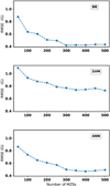 |
Fig. 1. Root mean square inversion errors (RMSE) in units of Gauss, as function of the number of MZSs included in the training; the inner legend in each panel indicates the employed regression model (see text for details). The inversion sample consist of 1500 MZSs. |
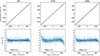 |
Fig. 2. Performance of the regression models when 300 MZSs were considered during the training process. The X axis for all panels corresponds to the original value of Heff for each of the 1500 MZSs. In the upper panels the Y axis represents the predicted values of the inversions, while in the lower panel it corresponds to the inversion errors in units of Gauss. The red line in the upper panels represents a one-to-one relation. |
For this purpose, we first used only 50 MZSs to train the algorithms and then we tested each regression model inverting a representative set of 1500 MZSs. We then repeated the exercise but increasing the number of MZSs used in the training process by steps of 50 until reaching a maximum of 500. The performance for all the regression models is shown in Fig. 1. The three models showed similar results, obtaining very accurate determinations of the Heff even when we considered a very small number of MZSs in the training process: using 100 MZSs, the obtained RMSE is inferior to 1 Gauss. The general tendency is that the errors decrease smoothly as we increase the number of MZSs employed in the training. Based on these results, we have decided that training the algorithms with 300 MZSs is sufficient for a proper determination of the stellar longitudinal magnetic field. Therefore, hereafter all the inversion tests are performed using 300 MZSs in the training process. In Fig. 2 we show the individual inversions of the 1500 MZSs for the three regression models.
The excellent results of Fig. 2 show the great utility of the employment of machine learning algorithms in the inference of Heff from the MZSs. As comparison, in Paper I we constructed 7500 spectra models and the RMSE of those inversions was 3.95 G, while with the best regression model (BR) we now obtain a RMSE of 0.41 G requiring only 300 spectra models. In other words, using this regression model the accuracy of inversions is increased by one order of magnitude, and at the same time the required time to synthesise the stellar spectra models (number of MZSs) is reduced by a factor of 25. It is important to note that the required time for the training of the algorithms is very fast: using a single processor, the cpu-time required was of 1, 5, and 120 s for the BR, SVM, and ANN regressors, respectively; moreover, in the case of BR and the ANN, the time can be reduced since the training process is parallelized.
Unfortunately, the effectivity of the regression models is considerably reduced when noise is taken into account. To illustrate this, we repeat the same exercise of Fig. 2 but this time including five different noise levels in the MZSs. The noise level (see Fig. 3) is quantified as the standard deviation of the noise divided by the standard deviation of the noise-free MZSs. In Fig. 4 we show the inversion results only for the BR model, which was the best regressor for the case of ideal MZSs without noise. (We note that our definition of the noise level is consistent with the work of Carroll & Strassmeier 2014, allowing us to make a proper comparison of the results below.)
From the results of Fig. 4, it is clear that for the inversion of noise-affected MZSs, the case corresponding to real data, the predictions are no longer good enough, even for the lowest noise level. For these tests, the training process was performed using noise-affected MZSs (with their respective noise levels), because in the alternative case – training with noiseless MZSs –, the errors were even slightly higher. Furthermore, it is also worth noticing that we have verified that the number of MZSs to be included in the training process does not depend on the noise levels, that is, to consider 300 MZSs in the training process is good enough for all noise levels.
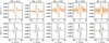 |
Fig. 3. In both upper and lower panels, the dashed line represents the original (noiseless) MZSs. The solid line in the upper panels corresponds to the noise-added MZSs; on top of each column are indicated the levels of noise. In the lower panels, the solid lines represent the cleaned MZSs. |
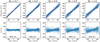 |
Fig. 4. Inversions of noise-added MZSs using the BR model. The different noise levels (NL) added to the MZSs are indicated at the top of the upper panels. The X and Y axes are the same as in Fig. 2 |
Based on the obtained results when noise is included, we propose a two-step process to improve the efficiency of the MZS inversions. These two steps consist in MZS noise cleaning and an iterative inversion methodology.
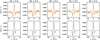 |
Fig. 5. Iterating the cleaning process considering one given MZSs and the same noise level. The solid and dashed lines have the same significance as in Fig. 3. As shown in the bottom panels, at each iteration, the cleaned profiles show small but different deviations from the original noiseless profile. |
3.2. Denoising profiles with principal components analysis
To facilitate the analysis of observed data, it is desirable to apply some noise treatment in order to give more credibility to the results. In the case of stellar spectropolarimetric data, the establishment of the multi-line (LSD or MZS) profiles is already a pre-processing step of the data analysis. However, the multi-line profiles are also affected by noise, which in turn degrades the accuracy of the inversions. Therefore, we subsequently use the term noise treatment to refer to any process applied to the multi-line profiles in order to deal with the noise problem.
Noise treatment, in this sense, can be implemented using for example either of the two following approaches. On the one hand, the Sparse Representation of data samples has recently begun to be implemented in the analysis of solar and stellar spectropolarimetric data with very good results (Asensio Ramos & de la Cruz Rodríguez 2015; Carroll & Strassmeier 2014). On the other hand, the principal components analysis (PCA), first introduced by Rees et al. (2000) for the study of solar magnetic fields, is a more commonly employed technique in the analysis of both, solar and stellar spectropolarimetric data. Both approaches implement a sort of space dimensionality reduction allowing to diminish the impact of the noise in the retrieval of the model parameters.
We employ PCA to perform “noise cleaning” of the MZSs: In the previous section we decided to use 300 MZSs for the training of the regression algorithms. By applying the Singular Value Decomposition to this same set of MZSs we obtain in turn 300 eigenvectors. It is well known that the eigenvectors are a mathematical base of the original set of MZSs, such that any MZSs can be obtained as a linear combination of those eigenvectors (e.g. Golub & van Loan 1996). Nevertheless, it is also possible to consider not the entire set of eigenvectors but only the first ones, because in fact the first eigenvectors are those that contain most of the useful information about the original MZSs (e.g. Paletou 2012). Accordingly, we considered only the first ten eigenvectors to perform noise cleaning:
where αi denote the scalar coefficients and evi the eigenvectors. The coefficients can be obtained through a dot product between each eigenvector and the MZS.
In Fig. 3, we illustrate the cleaning process of MZS profiles considering the same five levels of noise previously used (from 0.2 to 1.0 in steps of 0.2). The solid lines in the upper panels correspond to the noise-added profiles, while in the lower panels they represent the respective cleaned profiles. As comparison, the dashed lines in both upper and lower panels correspond to the original noise-free profiles. The noise-cleaning process can be seen to work well, even for the highest noise level. However, as expected, the higher the noise level, the greater the difference between the original and the cleaned MZSs.
We applied the described process to the full set of 1500 MZSs and repeated the same inversion test of Fig. 4, but this time implementing noise cleaning prior to the inversion of the profiles. Surprisingly, the results are not as good as expected, being only slightly better than for the case without the cleaning process, as shown in Table 1. For this reason, we propose a complementary step in the data analysis to improve the inversion efficiency.
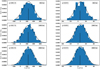 |
Fig. 6. Two examples of the iterative inversion process; the original values of Heff are 238.2G (left panels) and 5.2G (right panels). Each histogram shows the inversion distributions considering different numbers of iterations (indicated in the upper right corner). The upper left legend in each histogram indicates the centroid of the fitted normal Gaussian distribution, which would correspond to the inferred value of Heff in each case. |
Comparison of the RMSE for inversions performed when considering a noise-cleaning process of the profiles and when not.
3.3. Iterative inversion process
Let us consider only one given MZS from which we would like to infer Heff, and let us also consider a given fixed noise level, for example 0.4. In the previous section we showed how to perform noise cleaning of the profiles. We now consider a scenario in which we could repeat this process several times. For each iteration, the random noise will differently affect the MZS and subsequently the noise-cleaned profiles will all be slightly different. In Fig. 5 we illustrate how the cleaned profiles at each iteration differ from the original noise-free profile. For example, the maximum amplitude for the bottom-left cleaned profile is higher than the original one, contrary to the bottom-central cleaned profile where the maximum amplitude is inferior to the original one. These differences, although very small, are enough to produce a different result when inferring the longitudinal magnetic field. Nevertheless, we know that all the cleaned profiles have the same origin in the sense that all were established from the same noiseless data (dashed lines in Fig. 5). It is therefore expected that the inversions derived from these cleaned profiles will be close to the real value of Heff, and in fact they are, showing a distribution centred around the original value of Heff.
To illustrate our proposed methodology, in Fig. 6 we show two examples of iterative inversions. We have considered two MZSs, one with an Heff of 238.2G (left panels) and one with a much weaker magnetic longitudinal field of 5.2G (right panels). From top to bottom, the three panels show how the inversion distributions vary with the number of iterations: the larger the number of iterations performed, the more the histograms will approximate a normal Gaussian distribution (solid line in black). The centroid of the fitted Gaussian distribution, indicated with a vertical line, corresponds to the inferred value of Heff in each histogram.
In order to more carefully inspect the dependence of the results on the number of iterations, we tested the proposed inversion process using the full set of 1500 MZSs. Additionally, it is interesting to compare the performance of the three regression models introduced above. We recall that we are considering the same noise level of 0.4 for all the iterations and for all the MZSs. The RMSE of the inversions for the full set of profiles as a function of the number of iterations is shown in Fig. 7. All three regressor models show very similar behaviour, with a considerable improvement of the results especially for the first hundred iterations: When no iteration is applied, the RMSE are 24.6, 29.7 and 26.3 G for the BR, SVM, and ANN, respectively, and after 100 iterations the RMSE is reduced to 16 G for the three models, and at 1000 iterations the RMSE is of only 6 G. After around 1000 iterations, the improvement of the inversions becomes restrained. With the present results, we consider that applying 3000 iterations is good enough for the adopted inversion strategy.
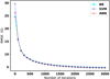 |
Fig. 7. Performance comparison of the three regression models as a function of the number of iterations when considering a noise level of 0.4. The performance of the three regressors is almost identical. |
Now, concerning the incertitude associated with our measurements of Heff, in principle, it is possible to obtain an error estimation based on the histograms of Fig. 6. Nevertheless, by doing this, we would be highly overestimating the errors: The standard deviation of the fitted Gaussian distribution for the bottom-left panel is 160 G, but in fact the error is much smaller, being of only 4.1 G. Similarly, an overestimation of the error is also obtained in another example from Fig. 6, in the bottom-right panel, where the standard deviation of the fitted distribution is 13.8G but the real error is only 1.2 G. Therefore, in order to obtain realistic estimations of the errors, we next proceed to inspect the inversions over the full sample of 1500 MZS.
3.4. Characterising the technique
We now show the performance of our proposed method considering different noise levels; we tested the inversions using the same set of 1500 MZSs as before, and in all cases we applied 3000 iterations. To quantify the accuracy in the results we have employed the mean absolute percentual error (MAPE), defined as:
Additionally, in order to underline the importance of including a noise treatment in the analysis of spectropolarimetric data, which in our case is done through the noise cleaning of the MZSs followed by the iterative inversion procedure, we also included the results from inversions performed when the profiles were inverted without any noise treatment, which we labelled as single inversions.
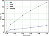 |
Fig. 8. Response of the MAPE of the inversions considering different noise levels. Each of the three regression models, as well as the case of single inversions, are indicated in the inner legends. |
In Fig. 8, we show the variation of MAPE as a function of the noise level. The three regressor models (BR, SVM, ANN) have the same performance as a function of the noise level: When no noise is included, the MAPE is extremely low (0.1%), but the inclusion of even a very small noise level of 0.1 leads to a (relatively) considerable increase of the MAPE (4%). However, the precision of the inversions for the models will then only decrease moderately to finish with a MAPE of 11% for the highest noise level of 1. Finally, the case of traditional inversions – noted simple by the line with square symbols –, is the most affected one, varying from 13% for the lowest noise level of 0.1 up to 47% for the highest noise level of 1.
One conclusion from this test is that with our proposed methodology – PCA noise cleaning combined with iterative inversions –, the three regression models are robust methods to determine Heff from MZSs that are affected by noise. Another important conclusion is that the single inversions are highly affected by noise, the respective errors being much higher than those obtained with any of the regression models. This is particularly evident for the case with the highest noise level (unity), where the MAPE of the single inversions can reach almost 50%, while for all three regressors, for this same noise level, the MAPE is close to 10%.
Similar results have previously been presented in Carroll & Strassmeier (2014). In this work the noise treatment is done adopting a sparsity representation of the data using an Ortogonal Match Pursuit (OMP) algorithm. In Fig. 10 of that article, the authors presented an analogous test to the one discussed here, comparing the inversions of noise affected profiles using the OMP approach with the ones obtained using the traditional centre-of-gravity (COG) method. The latter, is nowadays the method habitually employed when measuring Heff from real data and it is relevant in the sense that it does not consider any noise treatment. The authors have found that when considering a noise level of 1, and using the COG method, the MAPE is close to 50% (the same as in our single case), while using the OMP approach, the MAPE decreases to less than 20%. Both results, theirs and ours, highlight the importance of implementing a noise treatment in the inversion of polarised multi-line profiles.
The iterative process described in this section is a time-expensive step in our approach since it takes 3.75 h using eight processors in parallel. Nevertheless this relatively long time is required in order to achieve the precision errors shown in Fig. 8, and of course this time can be reduced if more processors are available.
4. Applying the method to real data
4.1. HD 190771
In this section we apply our method to real data. We have obtained from the public database PolarBase spectropolarimetric data of two cool solar-like stars, with very similar physical properties to the Sun. The first is HD 190771, whose atmospheric parameters are: Teff = 5834 ± 50 K, log g = 4.47 ± 0.03, M = 0.96 ± 0.13 M⊙, M/H = 0.14 and v sin i = 4.3 km s−1 (Valenti & Fischer 2005). For the synthesis of the stellar spectra, we took as starting point the closest model of the grid of Atlas9 atmospheric models (Teff = 5750 K, log g = 4.5 and M/H = 0.0), to then extrapolate to the exact values of Teff, log g and metallicity (see for example, Castelli 2005).
The synthesis of the spectra covered a wavelength range of 369–1010 nm in steps of 1 km s−1. As mentioned in Paper I, when constructing the MZSs our only criteria for the line selection is a minimum ratio of line depth to continuum, which for this work we have fixed > 0.1, resulting in a total number of individual lines of 23 172. The established MZS for the intensity, circular polarisation, and null profiles are shown Fig. 9.
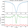 |
Fig. 9. From top to bottom: MZS profiles in intensity, circular polarisation, and null in the reference frame of the star. The central region, determined by the vertical lines, defines the rotational span velocities for this star in the Doppler space, from –16 to 16 km s−1 . |
 |
Fig. 10. Examples of MZS profiles obtained for the HD 190771 data (solid lines) and the respective noised-cleaned MZSs (dashed lines). The shape variations of the MZSs are similar to those in the synthetic case showed in the upper panel of Fig. 5. The dashed vertical lines determine the region employed in the inversion of the MZS profiles. |
The next step is to fit the observed broadening for the intensity Stokes profile. For this propose, we set as free parameters the projected rotational velocity of the star (v sin i) and the microturbulence velocity (ξ): We calculated a sample of 50 stellar spectra varying v sin i = [0.5,10] and ξ = [0,5] km s−1. We then trained an algorithm to simultaneously predict both parameters, obtaining as best fit values v sin i = 5.97 and ξ = 2.49 km s−1. In Fig. 11 we show the obtained fit of the synthetic profile to the observed one. In the adjustment of the intensity MZS profile, we are considering that all the other broadening processes, such as the magnetic, instrumental, or macroturbulent ones, can be well represented by the interplay between only these two free parameters. For this reason, the values of v sin i and ξ derived from this fitting are not real measurements of these two physical parameters.
In summary, we use an optimal atmospheric model (T eff = 5834 K, log g = 4.47, M/H = 0.14, v sin i = 5.97 km s−1 and ξ = 2.49 km s−1) to synthesise a set of 300 MZSs that we use to train the regression algorithms and to subsequently determine Heff for this star.
In order to follow a consistent MZS inversion procedure with our previous tests, we are required to determine the standard deviation of both the noise-free MZS (σMZS) and the noise (σnoi). The latter was determined using the edges of the circular MZS profile – indicated by the dashed vertical lines in Fig. 9 –, because in these regions there is only noise. For the former, we considered only the central region where the polarised signature is present. We then applied a noise-cleaning process to the polarised MZS as described in the previous section. Once we had obtained the cleaned MZS, we calculated the standard deviation from this noise-free profile. Finally, the noise level is determined as before, NL = σnoi/σMZS, obtaining a value of 0.15.
In order to apply the iterative inversions procedure, in each of the 39 echelle orders we added random white noise to the observed circular polarised spectra. The amplitude (Ai) of the added noise in each order is different, and is given by

where  is the standard deviation of the circular polarised spectra in the i-order, and α is a constant factor for all orders. It is through the value of α that the NL can be controlled in the MZS after the addition of random white noise. In Fig. 12 we show how the noise level of the MZSs varies as a function of the α value for this particular observation of HD 190771: For very low values of α – corresponding to high amplitudes in the added noise –, the NL is very high, but as α increases the NL decays very quickly, finally becoming stable at around NL ∼ 0.15, which corresponds to the noise level of the MZS when no noise was added. In this plateau phase of the NL, corresponding to α values from 0.3 to 2, we are interested in the minimum (α = 0.3), because the lower the value of α the higher the added noise, that is, the higher the variations in the iterative establishment of MZS profiles. In Fig. 10, we show some examples of the of MZS profiles for the HD 190771 data considerig α = 0.3.
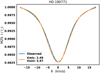 |
Fig. 11. MZSs in intensity for the data and the best fit model considering as free parameters v sin i and ξ (both in units of km s−1). |
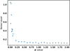 |
Fig. 12. Variation of the noise level of the MZSs as a function of the α value used in Eq. (13); see text for details. |
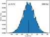 |
Fig. 13. Histogram of the inversion profiles for the star HD 190771, from which we determined a value of Heff = −6.3G. The regressor algorithm employed in the inversions is the BR. |
Finally, we considered 3000 iterations to produce the histogram of the inversion results. In Fig. 13 we show the distribution of the inversions, as well as the fit of the normal Gaussian distribution, from which we derived a value of Heff = −6.3 ± 0.3 G. Using the same dataset, Marsden et al. (2014) reported a value of Heff = −9.8 ± 0.3 G.
The value of the error in our measurement of Heff is based on the MAPE results of Fig. 8. Considering that in our inversions we employed the BR regressor and given that the noise level of the data is 0.15, this corresponds to a MAPE close to 5%, that is, an error of ±0.3 G. It is worth noticing that the same error is reported by Marsden et al. (2014) despite the fact that in the inversion of the LSD profile, the authors do not implement any noise treatment. As a reference, for the same NL of 0.15, the MAPE associated to the single case (inversions without noise treatment) is 15%, that is, the error should be around ±1.5 G. It therefore seems that the errors reported by classical techniques that do not consider noise treatment could be seriously underestimated.
If we now consider the estimation that we found of 1.5G for the error in the LSD measurement of Heff, then it turns out that the value of Heff reported by Marsden et al. (2014) and the one we found, would be in agreement at a difference of 2σ. On the contrary, if we consider the error of 0.3 G reported by the authors, then the difference could not be explained by the incertitudes associated with the measurements, and in this case the discrepancies in the results deserve a much deeper analysis, which is beyond the scope of the present study.
4.2. HD 9472
The second example is the star HD 9472, whose atmospheric parameters are Teff = 5867 ± 44 K, log g = 4.67 ± 0.02, M = 1.29 ± 0.19 M⊙, M/H = 0.0 and v sin i = 2.2 km s−1 (Valenti & Fischer 2005; Marsden et al. 2014).
We followed the same procedure as in the previous case, taking as point of departure the closest atmospheric model from the Atlas9 grid, namely, Teff = 5750 K, log g = 4.5, and M/H = 0.0, to then extrapolate to the exact values of T eff and log g. Adopting the same threshold of the line-depth to continuum as before (>0.1), the total number of individual lines is 23 895 for this star. We then established the MZSs, shown in Fig. 14.
The subsequent step was to reproduce the observed broadening in the intensity Stokes MZSs. We obtained as best fit values v sin i = 5.08 and ξ = 1.81 km s−1, which produced, as in the previous case, a very good fit between the synthetic and the observed profiles, as showed in Fig. 15.
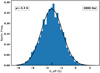 |
Fig. 17. Histogram of the inversion profiles for the star HD 9472, from which we determined a value of Heff = −3.3 G. The regressor algorithm employed in the inversions is the BR. |
The NL was then calculated for the circular MZS, obtaining a value of 0.19. We subsequently inspected the variation of the noise level as a function of the amplitude of the random noise added to the echelle orders, allowing to determine that setting α = 0.4 corresponds to MZSs with the same NL as the original data of 0.19; see Fig. 16. Finally, we iteratively established 3000 MZSs to consequently fit a Gaussian distribution to the histogram of the inversions, shown in Fig. 17. The centroid of the fitted distribution corresponds to a value of Heff = −3.3 ± 0.2 G, which in fact is almost the same as the one reported by Marsden et al. (2014) using the same data: Heff = −3.5 ± 0.4 G. Once more, it seems that the error reported by the authors is underestimated: based on Fig. 8, for this noise level the error should be around 17%, that is, 0.6 G.
5. Conclusions
We have presented a new study related to the measurement of stellar longitudinal magnetic fields, from high-resolution spectropolarimetric data, analysing multi-line profiles. Our main goal was to develop a general method which is neither constrained by the regime of validity of the weak field approximation nor by the line autosimilarity normally assumed in the classical methods employed nowadays in the measurement of Heff.
Our technique is therefore based on a theoretical radiative transfer approach where we produced a synthetic set of Stokes profiles, each one corresponding to a different configuration of the magnetic fields over the stellar surface. Considering the best possible scenario of noise-free spectra, we have shown that the use of MLA is a key step to reduce the number of synthetic profiles required for acceptable accuracy in the correct determination of Heff: With the use of MLA and considering only 50 stellar spectra, we obtained a better value of the RMSE for the inversion results than when we considered 7500 spectra and the inversion strategy was based on a look-up table, that is, no MLA was applied (Ramírez Vélez et al. 2016).
We also showed that the results are considerably degraded when noise is included; nevertheless this is not restricted to the MLA but applies to any method dealing with the inversion of noise-affected profiles or signals. We therefore proposed data noise pre-processing consisting of two steps: 1) Using PCA to perform noise-cleaning of the multi-line profiles and 2) an iterative inversion procedure. Applying this data analysis process, we achieved considerable improvement of the inversion accuracy, confirming that it is desirable to include a noise treatment in the analysis of multi-line profiles in order to get more confidence in the derived values of Heff. Very similar results in terms of the impact of noise in the inversion of multi-line profiles were independently found by Carroll & Strassmeier (2014).
We implemented our inversion technique to real observations of two stars. In order to similarly apply the MLAs to the observed data set (i.e. as closely as possible as in the case of synthetic spectra), we first needed to reproduce the observed broadening in the intensity profile. We allowed the variation of two physical parameters for this propose, namely v sin i and ξ, and we obtained very good fits, as shown in Figs. 11 and 15. Of course, the values of these two parameters lack any physical interpretation because we are assuming that all other broadening mechanisms (e.g. magnetic, instrumental or any other) can be well represented by considering only v sin i and ξ as adjustable parameters.
Therefore, the atmospheric model employed for the analysis of each star consisted in the exact values of Teff, log g, and metalicity – reported by other authors –, in addition to the values of v sin i and ξ. Once these five atmospheric parameters were defined, we synthesised a set of 300 polarised stellar spectra that in turn were used to train the MLA. One final step was to reproduce the iterative inversion methodology implemented in the synthetic tests. For this purpose, we added random white noise to each order of the echelle spectrum. The amplitude of the added noise in each order is different and is controlled by one free paramter, labelled α in Eq. (13). It is through the value of this parameter that it was possible to keep a constant noise level in the MZSs established for the iterative inversions. Finally, considering the same number of iterations in the case of real data as that used in the tests, we fitted a Gaussian normal function to the distribution of the inversion results. The centroid of the Gaussian distribution determines the value of Heff for each dataset (Figs. 13 and 17).
We used two stars as test cases to illustrate the direct application of the proposed methodology to real observations, and in this sense, it is beyond the scope of this work to compare the measured values of Heff with our technique with the ones obtained by other methods. We will proceed to the comparison of the values of Heff obtained with classical methods versus ours in a forthcoming article. However, what we can highlight here is the fact that the uncertainties reported in the measurement of H eff from the LSD profiles are most likely underestimated. Asensio Ramos & Petit (2015) recently presented a method to establish and analyse LSD profiles under a Bayesian framework. One of the advantages of this approach is that it can estimate the intervals of credibility at each velocity point of the LSD profiles. Unfortunately, although the authors applied their method to three different stars, they did not report the respective measurements of Heff, preventing the comparison of their estimation of errors with other techniques. As far as we know, no other work has addressed a detailed study on the expected uncertainties associated with the measurements of Heff from noise-affected LSD profiles.
The most relevant aspect of the work presented here is not that we have included estimations of the uncertainties in the measurements of Heff, but the fact that we have introduced a new methodology for the analysis of polarised multi-line profiles – including a radiative transfer theoretical framework in the synthesis of the Stokes profiles –, using a strategy based on machine learning algorithms. We expect to apply our data analysis method to stars other than solar-type in upcoming studies.
Acknowledgments
We are very grateful to the whole group of Laboratorio de Cómputo Inteligente del CIC-IPN2 for very constructive and illustrative discussions about machine learning methods. We would also like to express our acknowledgement to the anonymous referee for their comments, which helped to improve the clarity of this work. JRV acknowledges support grants from CONACYT 240441 and SUPERCOMPUTO – LANCAD-UNAM-DGTIC-326. Thanks go to AdaCore for providing the GNAT GPL Edition of its Ada compiler.
Appendix A: Hyperparameters for each regressor
For the definition of each of the hyperparameters listed below, we refer the reader to Scikit-learn user guide. For consistence, we labelled each parameter following the mentioned guide3
A.1. Bayessian Ridge
BayesianRidge(alpha_1=1e-06,alpha_2=1e-06, compute_score=False, copy_X=True, fit_intercept=True, lambda_1=1e-06, lambda_2=1e-06, n_iter=300, normalize=False, tol=0.001, verbose=False)
A.2. Artificial Neuronal Network
MLPRegressor(activation=“identity”, alpha=0.05, batch_size=“auto”, beta_1=0.9, beta_2=0.999, early_stopping=False, epsilon=1e-08, hidden_layer_sizes=(100,), learning_rate=“constant”, learning_rate_init=0.001, max_iter=10000, momentum=0.9, nesterovs_momentum=True, power_t=0.5, random_state=25, shuffle=True, solver=“lbfgs”, tol=1e-08, validation_fraction=0.1, verbose=False, warm_start=False)
A.3. Support Vector Machine
SVR(C=50.0, cache_size=200, coef0=0.0, degree=3, epsilon=0.1, gamma=“auto”, kernel=“linear”, max_iter=-1, shrinking=True, tol=0.001, verbose=False)
References
- Angelou, G. C., Bellinger, E. P., Hekker, S., & Basu, S. 2017, ApJ, 839, 116 [Google Scholar]
- Armstrong, D. J., Kirk, J., Lam, K. W. F., et al. 2016, MNRAS, 456, 2260 [NASA ADS] [CrossRef] [Google Scholar]
- Asensio Ramos, A., & de la Cruz Rodríguez, J. 2015, A&A, 577, A140 [NASA ADS] [CrossRef] [EDP Sciences] [Google Scholar]
- Asensio Ramos, A., & Petit, P. 2015, A&A, 583, A51 [NASA ADS] [CrossRef] [EDP Sciences] [Google Scholar]
- Bellinger, E. P., Angelou, G. C., Hekker, S., et al. 2016, ApJ, 830, 31 [NASA ADS] [CrossRef] [Google Scholar]
- Carlin, B. P., & Louis, T. A. 2008, Bayesian Methods for Data Analysis (CRC Press) [Google Scholar]
- Carroll, T. A., & Strassmeier, K. G. 2014, A&A, 563, A56 [NASA ADS] [CrossRef] [EDP Sciences] [Google Scholar]
- Castelli, F. 2005, Mem. Soc. Astron. It. Suppl., 8, 25 [Google Scholar]
- Castelli, F., & Kurucz, R. L. 2004, ArXiv e-prints [arXiv:astro-ph/0405087] [Google Scholar]
- Chang, C.-C., & Lin, C.-J. 2011, ACM Trans. Intell. Syst. Technol., 2, 27 [Google Scholar]
- Davies, G. R., Silva Aguirre, V., Bedding, T. R., et al. 2016, MNRAS, 456, 2183 [NASA ADS] [CrossRef] [Google Scholar]
- Donati, J.-F., & Landstreet, J. D. 2009, ARA&A, 47, 333 [NASA ADS] [CrossRef] [MathSciNet] [Google Scholar]
- Donati, J.-F., Semel, M., Carter, B. D., Rees, D. E., & Collier Cameron, A. 1997, MNRAS, 291, 658 [NASA ADS] [CrossRef] [MathSciNet] [Google Scholar]
- Du, K.-L., & Swamy, M. 2014, Neural Networks and Statistical Learning (Springer), 15 [CrossRef] [Google Scholar]
- García-Floriano, A., López-Martín, C., Yáñez-Márquez, C., & Abran, A. 2018, Inf. Softw. Technol. [Google Scholar]
- Glantz, S. A., Slinker, B. K., & Neilands, T. B. 2016, Primer of Applied Regression & Analysis of Variance (McGraw-Hill Medical Publishing Division) [Google Scholar]
- Golub, G. H., & van Loan, C. F. 1996, Matrix Computations (Baltimore: Johns Hopkins University Press) [Google Scholar]
- Grunhut, J. H., Wade, G. A., Neiner, C., et al. 2017, MNRAS, 465, 2432 [NASA ADS] [CrossRef] [Google Scholar]
- Jefferies, J., Lites, B. W., & Skumanich, A. 1989, ApJ, 343, 920 [NASA ADS] [CrossRef] [Google Scholar]
- Kochukhov, O., Makaganiuk, V., & Piskunov, N. 2010, A&A, 524, A5 [NASA ADS] [CrossRef] [EDP Sciences] [Google Scholar]
- Marsden, S. C., Petit, P., Jeffers, S. V., et al. 2014, MNRAS, 444, 3517 [NASA ADS] [CrossRef] [Google Scholar]
- Mathys, G. 1989, Fundam. Cosmic Phys., 13, 143 [Google Scholar]
- Paletou, F. 2012, A&A, 544, A4 [NASA ADS] [CrossRef] [EDP Sciences] [Google Scholar]
- Pedregosa, F., Varoquaux, G., Gramfort, A., et al. 2011, J. Mach. Learn. Res., 12, 2825 [Google Scholar]
- Petit, P., Dintrans, B., Solanki, S. K., et al. 2008, MNRAS, 388, 80 [NASA ADS] [CrossRef] [MathSciNet] [Google Scholar]
- Petit, P., Louge, T., Théado, S., et al. 2014, PASP, 126, 469 [NASA ADS] [CrossRef] [Google Scholar]
- Ramírez Vélez, J. C., Semel, M., Stift, M., et al. 2010, A&A, 512, A6 [NASA ADS] [CrossRef] [EDP Sciences] [Google Scholar]
- Ramírez Vélez, J. C., Stift, M. J., Navarro, S. G., et al. 2016, A&A, 596, A62 [NASA ADS] [CrossRef] [EDP Sciences] [Google Scholar]
- Rees, D. E., & Semel, M. D. 1979, A&A, 74, 1 [NASA ADS] [Google Scholar]
- Rees, D. E., López Ariste, A., Thatcher, J., & Semel, M. 2000, A&A, 355, 759 [NASA ADS] [Google Scholar]
- Richards, J. W., Starr, D. L., Butler, N. R., et al. 2011, ApJ, 733, 10 [NASA ADS] [CrossRef] [Google Scholar]
- Rosenblatt, F. 1958, Psychol. Rev., 65, 386 [Google Scholar]
- Rumelhart, D. E., Hinton, G. E., & Williams, R. J. 1985, Learning Internal Representations by Error Propagation, Tech. Rep., California Univ. San Diego La Jolla, Inst for Cognitive Science [Google Scholar]
- Semel, M., & Li, J. 1996, Sol. Phys., 164, 417 [NASA ADS] [CrossRef] [Google Scholar]
- Semel, M., Rees, D. E., Ramírez Vélez, J. C., Stift, M. J., & Leone, F. 2006, in Solar Polarization 4, eds. Casini, R., & Lites, B. W., ASP Conf. Ser., 358, 355 [NASA ADS] [Google Scholar]
- Semel, M., Ramírez Vélez, J. C., Martínez González, M. J., et al. 2009, A&A, 504, 1003 [NASA ADS] [CrossRef] [EDP Sciences] [Google Scholar]
- Sennhauser, C., & Berdyugina, S. V. 2010, A&A, 522, A57 [NASA ADS] [CrossRef] [EDP Sciences] [Google Scholar]
- Sennhauser, C., Berdyugina, S. V., & Fluri, D. M. 2009, A&A, 507, 1711 [NASA ADS] [CrossRef] [EDP Sciences] [Google Scholar]
- Stift, M. J. 1975, MNRAS, 172, 133 [NASA ADS] [CrossRef] [Google Scholar]
- Stift, M. J. 2000, Peculiar Newlett., 33, 27 [Google Scholar]
- Stift, M. J., Leone, F., & Cowley, C. R. 2012, MNRAS, 419, 2912 [NASA ADS] [CrossRef] [Google Scholar]
- Tan, P.-N., Steinbach, M., & Kumar, V. 2005, Introduction to Data Mining (Pearson Addison Wesley), 769 [Google Scholar]
- Valenti, J. A., & Fischer, D. A. 2005, ApJS, 159, 141 [NASA ADS] [CrossRef] [MathSciNet] [Google Scholar]
- Vapnik, V. N. 1999, IEEE Trans. Neural Networks, 10, 988 [CrossRef] [PubMed] [Google Scholar]
- Verma, K., Hanasoge, S., Bhattacharya, J., Antia, H. M., & Krishnamurthi, G. 2016, MNRAS, 461, 4206 [NASA ADS] [CrossRef] [Google Scholar]
- Wade, G. A., Donati, J.-F., Landstreet, J. D., & Shorlin, S. L. S. 2000, MNRAS, 313, 823 [NASA ADS] [CrossRef] [MathSciNet] [Google Scholar]
- Wade, G. A., Neiner, C., Alecian, E., et al. 2016, MNRAS, 456, 2 [NASA ADS] [CrossRef] [Google Scholar]
- Yang, Y., & Zou, H. 2015, Stat. Comput., 25, 1129 [CrossRef] [Google Scholar]
All Tables
Comparison of the RMSE for inversions performed when considering a noise-cleaning process of the profiles and when not.
All Figures
|
Fig. 1. Root mean square inversion errors (RMSE) in units of Gauss, as function of the number of MZSs included in the training; the inner legend in each panel indicates the employed regression model (see text for details). The inversion sample consist of 1500 MZSs. |
| In the text | |
|
Fig. 2. Performance of the regression models when 300 MZSs were considered during the training process. The X axis for all panels corresponds to the original value of Heff for each of the 1500 MZSs. In the upper panels the Y axis represents the predicted values of the inversions, while in the lower panel it corresponds to the inversion errors in units of Gauss. The red line in the upper panels represents a one-to-one relation. |
| In the text | |
|
Fig. 3. In both upper and lower panels, the dashed line represents the original (noiseless) MZSs. The solid line in the upper panels corresponds to the noise-added MZSs; on top of each column are indicated the levels of noise. In the lower panels, the solid lines represent the cleaned MZSs. |
| In the text | |
|
Fig. 4. Inversions of noise-added MZSs using the BR model. The different noise levels (NL) added to the MZSs are indicated at the top of the upper panels. The X and Y axes are the same as in Fig. 2 |
| In the text | |
|
Fig. 5. Iterating the cleaning process considering one given MZSs and the same noise level. The solid and dashed lines have the same significance as in Fig. 3. As shown in the bottom panels, at each iteration, the cleaned profiles show small but different deviations from the original noiseless profile. |
| In the text | |
|
Fig. 6. Two examples of the iterative inversion process; the original values of Heff are 238.2G (left panels) and 5.2G (right panels). Each histogram shows the inversion distributions considering different numbers of iterations (indicated in the upper right corner). The upper left legend in each histogram indicates the centroid of the fitted normal Gaussian distribution, which would correspond to the inferred value of Heff in each case. |
| In the text | |
|
Fig. 7. Performance comparison of the three regression models as a function of the number of iterations when considering a noise level of 0.4. The performance of the three regressors is almost identical. |
| In the text | |
|
Fig. 8. Response of the MAPE of the inversions considering different noise levels. Each of the three regression models, as well as the case of single inversions, are indicated in the inner legends. |
| In the text | |
|
Fig. 9. From top to bottom: MZS profiles in intensity, circular polarisation, and null in the reference frame of the star. The central region, determined by the vertical lines, defines the rotational span velocities for this star in the Doppler space, from –16 to 16 km s−1 . |
| In the text | |
|
Fig. 10. Examples of MZS profiles obtained for the HD 190771 data (solid lines) and the respective noised-cleaned MZSs (dashed lines). The shape variations of the MZSs are similar to those in the synthetic case showed in the upper panel of Fig. 5. The dashed vertical lines determine the region employed in the inversion of the MZS profiles. |
| In the text | |
|
Fig. 11. MZSs in intensity for the data and the best fit model considering as free parameters v sin i and ξ (both in units of km s−1). |
| In the text | |
|
Fig. 12. Variation of the noise level of the MZSs as a function of the α value used in Eq. (13); see text for details. |
| In the text | |
|
Fig. 13. Histogram of the inversion profiles for the star HD 190771, from which we determined a value of Heff = −6.3G. The regressor algorithm employed in the inversions is the BR. |
| In the text | |
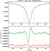 |
Fig. 14. As in Fig. 9, but for HD 9472. The star spans the Doppler space from –12 to 12 km s−1. |
| In the text | |
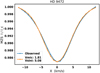 |
Fig. 15. As in Fig. 11, but for HD 9472. |
| In the text | |
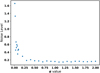 |
Fig. 16. As in Fig. 12, but for the data of HD 9472. |
| In the text | |
|
Fig. 17. Histogram of the inversion profiles for the star HD 9472, from which we determined a value of Heff = −3.3 G. The regressor algorithm employed in the inversions is the BR. |
| In the text | |
Current usage metrics show cumulative count of Article Views (full-text article views including HTML views, PDF and ePub downloads, according to the available data) and Abstracts Views on Vision4Press platform.
Data correspond to usage on the plateform after 2015. The current usage metrics is available 48-96 hours after online publication and is updated daily on week days.
Initial download of the metrics may take a while.