| Issue |
A&A
Volume 619, November 2018
|
|
|---|---|---|
| Article Number | A64 | |
| Number of page(s) | 12 | |
| Section | The Sun | |
| DOI | https://doi.org/10.1051/0004-6361/201732563 | |
| Published online | 08 November 2018 | |
Effects of resonant scattering of the Si IV doublet near 140 nm in a solar active region⋆
1
Research Center for Astronomy and Applied Mathematics, Academy of Athens, 4 Soranou Efessiou Str., Athens 11527, Greece
e-mail: cgontik@academyofathens.gr
2
Université Paris Sud, Institut d’Astrophysique Spatiale, UMR8617, 91405 Orsay, France
3
CNRS, Institut d’Astrophysique Spatiale, UMR8617, 91405 Orsay, France
Received:
29
December
2017
Accepted:
20
August
2018
Aims. In a previous study we analysed the C IV 1548.189 Å and 1550.775 Å lines observed with the Solar Ultraviolet Measurements of Emitted Radiation (SUMER), showing cases where the 1548.189 Å spectral profile was noticeably different from the 1550.775 Å one, profiles that we dubbed differentially shaped profiles. We explained this differential behaviour by an important radiative contribution, affecting multiple plasma motions happening at the instrument sub-resolution scale. In the present study we examine more general cases where radiative effects may contribute to the emission from the transition region of an active region. Here we analyse the lines Si IV 1393.757 Å and 1402.772 Å observed with the Interface Region Imaging Spectrograph (IRIS).
Methods. We study active region NOAA 12529, observed with IRIS on 18 April 2016. Using sorting techniques we selected individual profiles for which the intensity line ratio 1393.757 Å/1402.772 Å is significantly higher or lower than 2 and we also tracked differentially shaped profiles. We analyse the physical conditions that create these profiles and in some cases we estimate electron densities.
Results. We found more than 4000 individual profiles with line ratios higher than 2, about 500 profiles for which the line ratio is in the range 1.3–1.6, and 15 differentially shaped profiles. Line ratios higher than 2, are found along loops, and mostly at the y = 250 to 300″ part of the plage. There, we estimated the incident radiation and derived electron densities that can vary from 109 to a few times 1011 cm−3, depending on the plasma temperature. For the low line ratios, the sources are concentrated at the periphery of the active region plage, mostly along fibrils and present optical depths, τ, between 1.5 and 3. in most cases. The electron densities calculated from these Si IV profiles are comparable with electron densities derived using the O IV 1399.766 Å-1401.163 Å ratios.
Conclusions. We found that about 2.4% of the individual profiles for which we can perform a Gaussian fit present a line ratio higher than 2. In profiles with a high line ratio, the resonant scattering appears to be due to the combination of an average incident radiation field with a relatively low local electron density and not due to the vicinity of an ephemeral strong light source. As far as low intensity ratios are concerned, non-negligible optical depths are found at the edge of the plage, near the footpoints of fibrils that are oriented towards quiet Sun areas, where the electron density can be as high as (7 − 9) × 1011 cm−3 if we assume a plasma in ionization equilibrium.
Key words: Sun: transition region / line: profiles / line: formation
The movie associated to Fig. 3 is only available at https://www.aanda.org
© ESO 2018
1. Introduction
As far as the transition region between the chromosphere and the corona (CCTR) is concerned, because the temperature ranges from about 104 to 106 K, and densities from 1012 down to 109 cm−3, most diagnostics of the CCTR plasmas have relied until now upon the so-called “coronal approximation” (Seaton 1964), which evolved into the very efficient multilevel approach (see the latest versions of the atomic database CHIANTI, Dere et al. 1997; Landi et al. 2012; Del Zanna et al. 2015). These diagnostics rely upon the thermal-only formation of the lines, where electron collisions play the only role, (Mason & Monsignori Fossi 1994). This excludes the chromosphere itself where radiative transfer in non-Local Thermodynamic Equilibrium is effective in most lines and continua. This also excludes the upper solar corona where the main formation process of lines and continua is radiation scattering (resonance, Thompson scattering). In-between, the thermal formation is certainly valid in the regions of the CCTRs where the temperature and density are high enough on the one hand, and for lines which are optically thin on the other hand. However, radiative phenomena, such as resonant scattering, are known to be important in the cooler part of the CCTR (Judge & Pietarila 2004). Moreover, the importance of resonant scattering has been found in C III spectral lines emitted from eruptive prominences (Jejčič et al. 2017).
Observations with the Solar Ultraviolet Measurements of Emitted Radiation (SUMER; Wilhelm et al. 1995) on board the SOlar and Heliospheric Observatory (SOHO) in the C IV 1548.189 Å and 1550.775 Å have drawn attention to some inconsistencies in the usual “thermal” analysis of active regions (Gontikakis & Vial 2016).
Analysing a few complex profiles of the C IV doublet at 1548.189 Å and 1550.775Å, Gontikakis & Vial (2016) found intensity ratios of 1548/1550, higher than 2, which is the ratio of the oscillator strengths, while the spectral shape of the C IV 1548.189 Å profile was different from the spectral shape of the C IV 1550.775 Å profile (these profiles were called differentially shaped profiles).
The interpretation was that these anomalous profiles are emitted by plasma volumes that are nearby and below SUMER’s spatial resolution, while they have different line-of-sight (LOS) Doppler shifts and they are differently affected by resonant scattering (Gontikakis & Vial 2016). As will be explained later on in the text, when resonant scattering becomes important, the intensity ratio 1548/1550 is higher than 2.
Actually, such cases have already been noticed for example in the same C IV 1548.189 Å and 1550.775 Å line doublet by Lites & Cook (1979), who observed a flare with the NRL S082B slit spectrograph on Skylab on 9 August 1973, (see Fig. 1). The profiles during the flare had different shapes in the two lines.
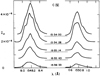 |
Fig. 1. Temporal evolution of C IV 1548.189 Å and 1550.775 Å line profiles during a flare, observed in August 1973 with S082B spectrograph on Skylab, (Fig. 1c from Lites & Cook 1979, p. 599, © AAS. Reproduced with permission). |
In a similar event, Gontikakis et al. (2013) show one more example of a small structure emitting C IV 1548.189 Å and 1550.775 Å with a line ratio higher than 2. There, resonant scattering dominates over thermal emission because of high incident radiation, caused by a near-by, simultaneous micro-flare. One more such example of resonant scattering influencing C IV lines emission is also found in Jordan et al. (1979). A more complex phenomenon, leading to the emission from a flare of linear polarized light is presented in Chambe & Henoux (1979). Resonant scattering is also essential in the case of prominences (Heinzel et al. 2015) where the quiet chromospheric incident radiation provides the input.
However, in the case where the scattering of some incident radiation plays an important role, it is very difficult to assess its spatial origin. The usual spectro-imaging implies the rastering of the slit which takes (at least) a few tens of seconds (in the case of SUMER) and has a good chance of missing the location of the flaring (small) region. Moreover, as pointed out by Gontikakis & Vial (2016), in the case of SUMER the radiative diagnostic may be complicated by the fact that the plane mirror allowing for the spectral scan is actually a non-negligible polarization analyser (Hassler et al. 1997). This last feature leads to a selective recording of the 1548.189 Å (polarized) line versus the 1550.775 Å line.
Another difficulty in the diagnostic of the CCTR plasma arises because the plasma is often affected by non-negligible optical thickness. The measurement of spectral line opacities in the transition region has been pursued with different techniques (Dumont et al. 1983; Fischbacher et al. 2002; Buchlin & Vial 2009). Recently, with the use of the Interface Region Imaging Spectrograph (IRIS mission; De Pontieu et al. 2014), more studies of opacity effects in the CCTR have been published (Yan et al. 2015). However, in active regions, the opacity of specific structures such as fibrils and dynamic fibrils (de Wijn & De Pontieu 2006; Tsiropoula et al. 2012) has being studied in chromospheric lines, such as Hα, but not in CCTR lines.
In the present work, we took advantage of the IRIS mission (De Pontieu et al. 2014), which has the triple properties of providing a very large database, an excellent time resolution, and negligible polarization effects to investigate more observations of individual complex profiles as well as profiles well described by a single Gaussian that are affected by resonant scattering or by opacity. Here we present an analysis of a number of observations in the Si IV 1393.757 Å and 1402.772 Å lines, which show the above-mentioned examples. The Si IV 1393.757 Å and 1402.772 Å lines form a doublet, like the C IV lines. The line ratio 1393.757/1402.772 is equal to 2 for the thermal optically thin case, higher than 2 under the effect of resonant scattering and lower than 2 when the plasma is optically thick.
Our paper is organized as follows: Sect. 2 presents the observations and the data treatment. Section 3 presents individual profiles influenced by resonant scattering or opacity as well as examples of anomalous profiles that are similar to the ones presented in Gontikakis & Vial (2016). Finally, Sect. 4 presents our conclusions.
2. Observations and data treatment
Active region NOAA 12529 was observed with IRIS on 18 April 2016. IRIS performed a raster starting at 01:14:09 UT and ending at 02:16:05 UT and recorded slit-jaw images. The raster field of view (FOV) was of (x,y) = (140.52″ × 182.3″) and was centred at (x,y) = (681.6″, 254.1″). Therefore this raster did not include the large sunspot of NOAA 12529, centred at (787″, 220″), which was included in the FOV in previous IRIS rasters (Guglielmino et al. 2018). The raster recorded the spectral lines of Si IV 1393.757 Å and 1402.772 Å (see CHIANTI database for the wavelengths) with an exposure time of 8 s. It also includes the spectral lines of C II 1334.535Å, 1335.710 Å and Mg II 2798.823Å, 2803.531Å. Figure 2a shows the intensity image of Si IV 1393.757 Å recorded with the raster. Some areas, such as the south-east, in the ranges of x = 620″ –640″ and y = 162″–240″ are composed of dark quiet Sun areas. A small bright loop is visible at (697, 323)″. The triangles, diamonds, and squares seen on the figure will be explained later in the text. Moreover, in Fig. 2a, the image was cleaned of cosmic rays after applying sorting techniques on the results of the Gaussian fit on the Si IV 1393.757 Å line.
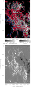 |
Fig. 2. Panel a: raster intensity image of the Si IV 1393.757 Å line. High 1393/1402 ratios are indicated with red triangles, blue diamonds indicate low line ratios, and green squares indicate differentially shaped profiles. Panel b: raster-like HMI/SDO magnetogram of the same region. |
In order to calibrate the dispersion axis, we computed Gaussian fits on the Fe II 1392.82 Å profiles, averaged along each of the 400 slit positions. The variation of the Doppler shift as a function of the slit position has a small correlation with the curve correcting the thermal and orbital variation and for the FUV band. The variation of the Fe II Doppler shift with time, after being smoothed, is of the order of ±0.7kms−1 , and is small relative to the Doppler shifts in which we are interested. Therefore, we used the averaged profile position out of our 400 profiles. The Fe II spectral lines are found to be redshifted by 1km s−1 , in comparison to cooler chromospheric spectral lines (Teriaca et al. 1999) such as the S I and Si I lines, which is very small for the purpose of our study. Therefore, we considered the Fe II 1392.82 Å line to be at rest. Using this wavelength scale, we estimated the Doppler velocities of the Si IV spectral profiles.
We performed single Gaussian fits of the Si IV 1393.757 Å and 1402.772 Å lines to perform intensity, Doppler, and line width maps of the FOV. For individual spectral pixels, where the profiles were complex and showed two or three spectral components, we applied double or triple Gaussian fits. For these complex cases we applied constraints in the fit procedure so that the Doppler shift and the Doppler width of each spectral component of the Si IV 1393.757 Å line were equal to the corresponding quantities of the Si IV 1402.772 Å line.
Our dataset also includes the spectral lines O IV 1399.766 Å and 1401.163 Å lines whose intensity ratio is sensitive to the electron density (Young 2015). These lines are very faint: the average peak intensity of the Si IV 1393.757 Å line over the whole image FOV is equal to 120 counts, while the average peak intensities of the O IV 1399.766 Å and 1401.163 Å lines are of two counts and six counts respectively. In the individual profiles there are many cases of negative values, probably because of errors in the pedestal correction of the data. We computed Gaussian fits over sets of O IV 1399.766 Å and 1401.163 Å spectral profiles, each set derived from the sum of 25 individual O IV 1399.766 Å and 1401.163 Å spectral profiles. These 25 profiles are selected from boxes of 5 × 5 spatial pixels, centred on selected spatial pixels where we analyse the co-spatial Si IV spectral line profiles. When binning the O IV profiles we ignored negative intensity values. For the selected averaged O IV profiles, we computed the 1399/1401 line ratios and derived electron densities according to the CHIANTI v.7 atomic database.
In this work, we are interested in individual profiles where the intensity line ratio of the Si IV 1393.757 Å total intensity over the 1402.772 Å total intensity is either higher than 2, which is the ratio of the oscillator strengths of the two spectral lines, or lower than 2. Moreover, we also examined cases of “differentially shaped profiles” where the individual profiles of Si IV 1393.757 Å have a different spectral shape from the Si IV 1402.772 Å profiles, recorded at the same time and spatial pixel.
In order to find the maximum number of profiles of the previous three categories, we applied different kinds of sorting procedures to the data. We applied these procedures to the parameters calculated from the single Gaussian fits. To keep a good statistic, we selected profiles for which the peak intensity of the Si IV 1402.772 Å line is higher than 30 counts. Moreover, the computed widths of the two lines should be larger than 1.6 spectral pixels since for widths larger than 1.6 we avoid many cosmic hits. More detailed sorting techniques were used for each case and will be described later on. There are no instrumental issues that can affect the intensity ratios of the two spectral lines, as long as we avoid the horizontal fiducial marks (Wuesler, priv. comm.). There is an imperfect background correction producing a 3–4 DN depression of the spectra, between approximately 1390 Å and 1395Å, for positions on the slit higher than 400 pixels (Liu 2017, priv. comm.). We checked whether this effect might produce line ratios artificially lower than 2 but this is not the case.
In anticipation of the thorough analysis of the three classes of profiles presented below, we built a movie available online, from the sequence of SJIs in the 1400 Å band recorded between 01:14:37 UT and 02:16:05 UT, where we implemented along the slit, at each raster time, symbols characteristic of the three classes as in Fig. 2a. The reader can refer to this movie when profiles and line ratios are discussed. Figure 3 shows one of these 98 images at 01:35:44 UT.
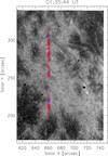 |
Fig. 3. Slit jaw image in the 1400 Å passband. Triangles, diamonds, and squares have the same meaning as in Fig. 2a. The positions indicated with these symbols correspond to spectral profiles recorded during the raster between 01:35:44 UT and 01:36:21 UT. Ninety-eight of these slit jaw images form a movie (available online). |
The two Si IV spectral lines form a doublet as they share a common ground level. The atomic transition of the Si IV 1393.757 Å line is 3s 2S 1/2 − 3p 2P3/2 while the one of Si IV 1402.772 Å is 3s 2S 1/2 − 3p 2P1/2 (see CHIANTI v.7 database). In the following, we will often represent the integrated over wavelength intensity, named total intensity of the 1393.757 Å line, as I13 and the total intensity of the 1402.772 Å line as I12.
Finally we also used 80 magnetograms from the Helioseismic and Magnetic Imager (HMI; Scherrer et al. 2012) on board the Solar Dynamic Observatory (SDO; Pesnell et al. 2012). These images have a 0.5″ spatial resolution, a cadence of 45 s and are recorded during the IRIS raster. For each exposure of the IRIS slit, we selected the magnetogram closest in time. Then, we kept the section of the magnetogram with the same FOV as the one observed by the IRIS slit position. We used all these slit-like magnetic images to compute a raster-like magnetic field map.
Figure 2b, shows the raster-like magnetic field image. The plage, found roughly in the range of x = 620–720″ and y = 200–270″ part of Fig. 2a, corresponds to positive unipolar magnetic regions, while in the western part of the plage we see negative polarities. A polarity inversion line lays roughly from (740″, 200″) up to (680″, 290″). Many loops visible in Fig. 2a connect positive with negative polarities. The brightest part of Fig. 2a at (720″, 215″) is found at a position of the polarity inversion line with a strong magnetic gradient.
3. Evidences of opacity and resonant scattering
3.1. Distribution of line ratios
In most cases the total intensity line ratio I13/I12 is equal to 2, which is equal to the ratio of the oscillator strengths of the two lines. This happens for an optically thin plasma. In Fig. 4, panel a shows a map of the I13/I12 total intensity ratio computed using single Gaussian fits. Black areas such as x = 620–640″, y = 170–240″, correspond to quiet Sun areas (dark in Fig. 2a) that have too few counts for a Gaussian fit to be computed. The black isocontours indicate ratios higher than 2.1 and white ones, ratios lower than 1.9. The blue areas with a line ratio below 1.9 are prominent in a large region with x = 610–660″ and y = 230–260″. A characteristic green coloured region of high ratio values is found within x = 620–660″ and y = 270–300″. Moreover, loop structures, such as that at (702″, 290″), present many cases with ratios higher than 2. This high ratio region corresponds to a bunch of loop structures in the intensity image (Fig. 2a), which lie across the polarity inversion line (Fig. 2b).
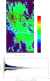 |
Fig. 4. Panel a: map of I13/I12 line ratio. The colours range from 1.6 to 2.3. The map is smoothed to 3 × 3 pixels. Black areas do not have a signal because their counts are too low. The white isocontours indicate the 1.9 values and the black isocontours the 2.1 ratios. Panel b: scatter plot of line ratio as a function of I13, the Si IV 1393.757 Å intensity. The black and blue plus signs represent the selected points with line ratios higher than 2. Black plus signs also indicate selected points with line ratios lower than 1.6 |
Panel b of Fig. 4 shows the scatter plot of line ratios as a function of Si IV 1393.757 Å intensity. The average of the line ratio of panel b is equal to 2, with a standard deviation of 0.28. The blue and black plus-signs for which the line ratios are higher than 2 are selected through different filtering procedures that will be presented in Sect. 3.2. Moreover, the plus-signs with line ratios smaller than 1.6 will be presented in Sect. 3.3 where we will discuss opacity effects.
3.2. Total intensity ratios higher than 2
We present cases of individual profiles, well represented with a single Gaussian fit (see Fig. 5), where the lines total intensity ratio r = I13/I12 is in the range of 2.1–3.
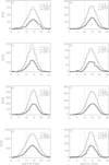 |
Fig. 5. Eight selected profiles of the Si IV 1393.757 Å (thin histogram line) and 1402.772 Å (thick histogram line) spectral lines where the lines ratio (r) is higher than 2. The data are represented with a histogram line while the Gaussian fit with a continuous line. The horizontal axis is in spectral pixels and the vertical axis in Data numbers. The dashed vertical shows the rest position for both lines. In each panel we show the total intensities line ratio. |
In order to find such profiles, we excluded profiles with low total counts and with low line widths, as we explained in Sect. 2. Moreover, the selected profiles are the ones where the line ratio calculated with the sum of counts is higher than 2, the χ2 is lower than three and where the relative variation of the widths of the two lines, Δω = |ω1393 − ω1402|/ω1393, is smaller than 0.2, where ω1393 and ω1402 are the Gaussian widths of the profiles expressed in spectral pixels. A small Δω indicates the good quality of the fit. We also had to avoid the fiducial lines where the intensities and the line ratios are modified. Finally we selected only the profiles for which the ratio minus the measurement error δr on the ratio is r − δr > 2. The δr is calculated using the error propagation method from the parameters of the Gaussian fits. The calculation of δr takes into account only the photon statistics. We found around 4000 such profiles (blue points in Fig. 4b). Figure 4, along with these 4000 profiles, shows roughly 16 500 points, with line ratios I13/I12 higher than 2.1, which were not selected because of the tight filtering of the data.
These individual profiles, indicated in Fig. 2a by triangles, cover a large part of the plage. The areas where these are most numerous correspond to the green coloured regions of Fig. 4a, such as in the area x = 620–660″, y = 270–300″, and the low-lying loops, (x = 688–716″, y = 290–296″). However, the diffusion points avoid the high intensity regions, such as x = 716–744″, y = 200–230″. We call the spatial pixels of these profiles “diffusion regions”, assuming that they are influenced by resonant scattering. These almost 4000 individual profiles represent roughly 2.4% of the raster individual profiles for which we can have a Gaussian fit. The triangles of the diffusion regions occupy different areas in Fig. 2a than the blue diamonds, which represent profiles showing the effects of opacity that will be presented in Sect. 3.3. However, there are many cases where triangles and diamonds are nearby. Such cases can be found at x = 650–670″, y = 195–250″, where one can see fibrils connecting the two dark quiet Sun areas of x = 620–650″, y = 190–230″ and x = 650–670″, y = 170–195″. In some cases, triangles and diamonds belong to close-by structures such as (x,y) = (650″, 195″) or maybe to the same structure (see movie accompanying Fig. 3).
In Fig. 5 the profiles are well represented with a single Gaussian fit. In each panel, the total intensity line ratio is indicated. In Fig. 5, panel g, we show that for this set of profiles the highest intensity profiles correspond the lowest line ratio (2.1), while the lowest intensity profiles (panels a and d) have the highest ratio values. This property is general as we will see in the following. The Doppler shifts of the almost 4000 diffusion profiles have the same statistical characteristics as the Doppler shifts distribution of the raster. Both Doppler shift distributions have average values close to 23 km s−1 and standard deviations close to 10 km s−1 for the raster distribution, and roughly 8 km s−1 for the diffusion profiles distribution.
In the following we simulate the incident radiation of the Si IV 1393.757 Å and 1402.772 Å lines at the diffusion points. This simulation proved to be time-consuming for the large number of diffusion regions. Therefore we further analysed only 443 diffusion profiles for which the χ2 of the Gaussian fit on the individual Si IV profiles is smaller than 1.4. In Fig. 4b, the blue plus signs represent the 4000 diffusion profiles and the black plus signs the 443 profiles of those selected for further study.
The diffusion regions have a spatial size of one pixel, which is of 0.33″ × 0.35″. We suppose that the diffusion regions are at an altitude h = 1–5″ from the surrounding area. Moreover, we suppose that the diffusion regions are illuminated by a spherical shell section, at the solar surface, defined from a circular area having a radius equal to  , where R is the solar radius, Dmax = 44.15″, and 98.42″ when h = 1″, and 5″, respectively. For each diffusion region, corresponding to a point P(xd,yd) on the image we computed the mean intensity
  , here written for the 1393.757 Å line:

Equation (1) computes the sum of the intensities multiplied by the corresponding solid angle dΩ = cos(γ(x,y)) dS/AS 2/μ(xd,yd) as seen from the diffusion point. The μ(xd,yd) is the cosine of the angle between the LOS and the perpendicular to the solar surface. Dividing dS by μ(xd,yd) provides an average correction of the individual surface projections on the image plane. For the selected points, μ(xd,yd) is in the range 0.5– 0.7. There, I13(x,y) is the emission line intensity, integrated over wavelength, as defined above at a position A(x,y), where (x,y) are the coordinates in image pixels, A(x,y) points are inside a circle with radius Dmax, centred at (xD,yD), as shown in Fig. 6, AS is the distance from A to S , dS = R2 sin αdαdϕ, where α is the angle at the solar centre C, and ϕ is the azimuthal angle around the SC axis. The angle γ(x,y) is the angle between the segment AS and the normal to the solar surface at point A(x,y). When A reaches B, the largest distance from where photons can reach S , γ = γmax = π/2 (see Fig. 6a). When we assume that the solar surface is of constant intensity, our calculation reduces to the geometrical dilution factor (Jejčič & Heinzel 2009). Numerically, we integrated Eq. (1) along concentric rings around each (xD,yD) point, the last ring being a circle with a radius equal to Dmax.
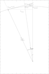 |
Fig. 6. Geometry of the incident radiation. A point S is at a distance h above the solar surface. The segment SC, where C is the solar centre, meets the surface at P(xD,yD). The point B is at the largest distance from where photons can reach S. The projected distance on the image is Dmax and θmax the angle at S. The point A(x,y) represents an intermediate position from where light can reach S , and γ is the angle between SA and the normal to the solar surface. |
For some (xD,yD) points where the surface included inside Dmax is larger than the raster FOV, we assumed that the missing points have the same intensity as the closest image edge. We performed this computation using two different methods for the selection of the incident intensities I(x,y).
In the first method, we used the total intensities I13(x,y) computed with Gaussian fits from the raster. We also computed an incident mean intensity  that we will use later in this section.
In the second method, we used the 1400 Å slit-jaw images. For each diffusion point (xD,yD), we selected the slit-jaw image that is closer in time to the slit recording. For each diffusion point there was a slit-jaw image recorded in a time shorter than 18.5 s from the slit recording. In Fig. 7 we show the results computed with the raster total intensities. Both methods gave almost the same results.
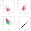 |
Fig. 7. Panel a: |


Panel a in Fig. 7 shows  computed for each diffusion region as a function of the line ratio for this region for an altitude h = 1″ (red triangles) and h = 5″ (black plus signs). Panel a shows that
  decreases as a function of the line ratio. This can be understood since Eq. (1) shows that
  has a higher contribution close to the (xD,yD) points. Therefore, if the (xD,yD) area belongs to a high density structure, this structure will produce high intensities, creating a high
  and producing an important radiative component at (xD,yD). On the other hand, (xD,yD) is connected to this high density structure that will cause a non-negligible collisional component so that the line ratio of the intensities emitted from (xD,yD) will be higher but close to 2.
Panel b shows the ratio of  over the intensity I13(xD,yD) at the diffusion region, as a function of the line ratio. We see that
  /I13(xD,yD) increases as a function of the line ratio. We will explain this finding later in this section.
In the following we show a method to compute the electron density ne at the diffusion regions using the mean specific intensities Jinc 13(λ), Jinc 12(λ) calculation as a function of the electron temperatures T. The mean specific intensities Jinc 13(λ), Jinc 12(λ) are computed using Eq. (1) where we used the spectral profiles instead of I13 and I12. The total intensities of the Si IV 1393.757 Å and 1402.772 Å lines are described theoretically by the equations (Gontikakis et al. 2013; Gontikakis & Vial 2016)
There, ni is the Si IV ion density which is assumed to be equal to the level 1 Si IV ion population as the two lines are resonant, and C12, C13, B12, B13 are the collision excitation coefficients and the Einstein coefficients for the lines, respectively, while L is the length of the LOS segment crossing the emitting volume. The collision excitation coefficients were computed using the rate_coeff Chianti v.7 routine. The  and
and  are the radiative excitation rates of the two lines, which are expressed as

The Jinc 13(λ) and Jinc 12(λ) incident mean profiles for the two lines are integrated over the solid angle. The ϕλ is the absorption profile. We computed the ϕλ using a Gaussian, centred at the Jinc 13(λ) profile, with a width depending on a temperature ranging from 40 000 K up to 2 × 10⁵ K and a non-thermal velocity of 10 km s−1.
Dividing Eq. (2) over Eq. (3) one gets the intensity ratio r on the left hand side and can express it as a function of the ratio X of the radiative term  over the collisional term Col13 = ni neC13, where
  , and we can derive the simple equation
In the above equation, from where we derive a X = X(r) function, we used the fact that C13/C12 = B13/B12 = 2, and we supposed that  , which is valid within 10% for our dataset. From Eq. (6) one can compute the electron density as
In order to derive electron densities from Eq. (7), first we expressed Jinc 13 in physical units, using the third version of IRIS radiometric calibration. In panel c of Fig. 7 we show computed electron densities as a function of the line ratio r. Black plus signs represent ne computed for a temperature and altitude of 4 × 10⁴ K, h = 1″ and red stars symbols to a temperature of 4 × 10⁴ K, and an altitude of h = 5″, while blue triangles and green squares correspond to an altitude of 1″ and temperatures of 8 × 10⁴ K, 2 × 10⁵ K, respectively. We see that, for a given r value, electron densities can vary up to a factor of five due to temperature variations while they present a variation of a few percent due to h variation. In all cases, ne decreases as a function of the line ratio by two orders of magnitude in panel c. This confirms our finding, that resonance becomes important in these areas because of a lower plasma density rather than because of an exceptionally high surrounding radiation field.
In panel d of Fig. 7, we show the ratio X as a function of the line ratio r. We see that for a line ratio between 2.3 and 2.4, which corresponds to a large fraction of our points, X is between .35 and .5, which means that the radiation term is not negligible when compared with the collisional one. This result depends only on the line ratio r.
We found the same results in Fig. 7 when we computed Jinc 13 with the intensities of the slit-jaw images as well as with the raster intensities. Indeed the slit jaw 1400 Å images have the same morphology as the raster intensity image. Therefore, the incident intensity is not influenced by a close-by, short-lived bright structure, not recorded by the raster.
Let us now discuss the results of panel b. According to Eq. (2), the ratio of the incident radiation over the total intensity of 1393.757 Å can be expressed also as
The first term in the denominator on the right hand side of Eq. (8) is proportional to  where we assumed that the hydrogen is fully ionized and that ni ∝ ne. As we can see in Fig. 7, panels a and c, the electron density has a higher dependence on the line ratio than Jinc 13. Therefore, the first term of the denominator of Eq. (8) decreases as a function of I13/I12. The second term in the denominator also decreases as a function of I13/I12 so that the ratio
  increases as a function of I13/I12 as we see in panel b, while we ignored the variations of L and T as a function of I13/I12. Therefore, from all the above calculations it seems that the high line ratio values depend on a decrease of the collision term rather than on a high value of the incident intensity.
In this study we stress the importance of the plasma temperature as a free parameter. Here we used three typical CCTR temperatures. Some authors (Dudík et al. 2014) found that because of departures from Maxwellian distributions, the Si IV lines could be formed at about 10 000 K (or below). Others (Schmit et al. 2014) found molecular absorption within Si IV profiles, a feature also related to low temperatures. At the end of this section we will present an effort to constrain the temperature values.
The individual profiles studied in this subsection are found in many places on the intensity image (Fig. 2a). They are found surrounding dark quiet Sun regions as well as along low-lying loops. Moreover, many profiles are found in the vicinity of small bright features. These small features have a size of roughly 0.3″ –1″. The slit-jaw 1400 Å movie (available online) corroborates these findings. The movie shows that along with the diffusion points related to fibrils and low-lying loops, many diffusion points are associated with moving small bright features. A comparison with chromospheric lines, such as Hα, and a careful and quantitative study of the slit-jaw time evolution is necessary to understand if these structures are associated with the bright grains described in Skogsrud et al. (2016). The cases of high line ratio profiles and their possible association with bright grains should be studied with a larger dataset.
3.3. Peak intensity ratios smaller than 2
We also selected profiles where the lines ratios I13/I12 are in the range of 1.3–1.6 (Fig. 4b) consequently ignoring about 15 000 profiles where the ratio is higher than 1.6 and lower than 2. We applied the same filters as for the resonant points to avoid spikes and noisy profiles. We found around 500 profiles with such low intensity ratios. These points are visible in the scatter plot of Fig. 4b. Figure 8 shows eight such profiles. The 1393.757 Å and 1402.772 Å profiles are shown centred at the same wavelength position along with a single Gaussian fit. In some cases the Gaussian fit represents well the profiles, as in Fig. 8 panels a and g, while in cases such as in Fig. 8 panels d and h the profiles show self-reversed profiles that the fit fails to represent. In Fig. 2a the selected profile positions are represented with blue diamonds. A large number of such points are found at the edge of low intensity regions, as for example at (x,y) (620, 250)″, at (640, 270)″, and at (650, 210)″. Self-reversed profiles have been found in the C IV 1548.189 Å line, to originate from plage regions observed at the limb (Lites et al. 1980).
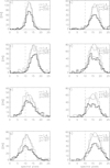 |
Fig. 8. Eight selected profiles of the Si IV 1393.757 Å and 1402.772 Å lines where the lines ratio is lower than 1.6. The data and the fit are represented as in Fig. 11. In each panel we show the total intensity line ratio (r) and the position of the profiles on Fig. 2a. The axes definitions are as in Fig. 5. |
In the slit-jaw movie (online), we also see that many of the low intensity ratio points belong to fibrils connecting the quiet Sun regions with the plage area. Bright blobs present proper motions along these fibrils towards or away from the quiet Sun areas.
We assumed that the profiles are optically thick, that the source functions of the two lines are equal S 13 = S 12, and that the source functions are constant along the LOS and independent of wavelength. The intensity is expressed as I13 0 = S 13(1 − exp(−τ13 0)), where I13 0 is the peak intensity and τ13 0 the central wavelength optical depth of the 1393.757 Å line. In this case, the profile is expressed by the function F(y) = 1 − exp(−τ0exp(−0.5y2)), where y = (λ − λ0)/ΔλD (see Dumont et al. 1983; Zirin 1988; Dere & Mason 1993). Here, λ0 is the reference wavelength and ΔλD the Doppler width (Dumont et al. 1983). We used two different methods to compute the τ13 0 at line centre. As a first method we computed the line ratio,
with the integrals being computed over the interval of interest. Solving Eq. (9) numerically (Dere & Mason 1993; Buchlin & Vial 2009), one gets a relation between τ13 0 and the total intensity line ratio. The computed τ13 0 values are in the range of 1.6–4.7. The second method was to compute a non-linear fit of the profiles with the F(y) function instead of a Gaussian one. We performed simultaneous fits of the Si IV 1393.757 Å and 1402.772 Å profiles adopting two constraints:
first that the Doppler shifts are the same for the two profiles, and second that τ13 0 = τ12 0/2. The fits using the F(y) are less successful than the Gaussian fits, as they have a higher chisquare. For 14 profiles, the χ2 based on the F(y) function over theχ2 based on a Gaussian function was lower than 1.75. For these profiles, the values of τ13 0 differ from 5% up to 80% from the values calculated with Eq. (9).
The reason is that the F(y) function has lower values in the wings that fail to describe the profiles. Therefore we can conclude that the assumption of a source function non-dependent on wavelength is not correct. However, the computed τ13 0 values are very often smaller than one so that the assumption of the source function being non-dependent on τ still holds.
Some pixels where we found low r values belong to elongated fibrils. We assumed that the observed structures are cylinders that we see almost perpendicular to the LOS. We performed Gaussian fits across the structures either along the slit or in fewer cases across the slit, and we assumed that the full width at half maximum (FWHM), which is defined as  times the Gaussian width, equals the structure length L along the LOS. In some cases the optically thick individual profile was at the centre of a very dark small location surrounded by fibrils from where it was not possible to deduce a spatial width, such as at (x,y) = (737″, 188″), (643″, 254″), or (674″, 315″) (see Fig. 2a). These points were not taken into account. We assumed that the structure is in ionization equilibrium and we used the definition of optical depth as in the equation (Mariska 1992, p.40)

where 0.8 is the hydrogen over electron ratio when hydrogen if fully ionized, l0 is the ion cross-section, Ab = 7.24 × 10⁻⁵ is the silicon abundance and f(T ) is the ionization equilibrium. The values for Ab, and f (T ) are taken from CHIANTI v.7. For the cross-section we used the formula by Mariska (1992) and we found values of 5 × 10⁻¹⁴ to 10−13 cm−2 due to the variation of the non-thermal velocities from 7 km s−1 to 20 km s−1. We assumed that the filling factor is equal to one. We used the symbol ne(op) for the electron densities derived with this method.
From Eq. (10) we derived electron densities for three temperatures: 80 000 K, for which we have the maximum Si IV ion population according to CHIANTI calculations, as well as 50 000 K and 125 000 K. For these last two temperatures, CHIANTI predicts that the Si IV ion density is roughly 0.1 times lower than the ion density for 80 000 K. We included these two temperatures as extreme cases under the assumption that the plasma is in a steady equilibrium. The electron densities presented in Fig. 9a for 80 000 K are between 5×10⁹ and 2×1011 cm−3. For the other two temperatures, the electron densities are higher by a factor of ten. In Fig. 9b we see the relation between τ13 0 and the structure widths. The measured optical depths are not correlated with the structure width, while the electron densities are proportional to the inverse of L.
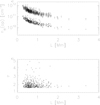 |
Fig. 9. Panel a: electron densities as a function of the structure width, calculated for three ionization equilibrium temperatures 50 000 K (plus signs), 80 000 K, (triangles) and 125000 K (squares). Panel b: opacity, computed using Eq. (10), as a function of the width. |
3.4. Comparison with electron densities computed using the O IV lines
The measurements of electron densities using the O IV 1399.766 Å and 1401.163 Å line give the possibility to check the robustness of our electron density measurements of Sects. 4.2 and 4.3 (De Pontieu 2017, priv. comm.).
As the O IV lines are faint, we binned 5 × 5 spectral profiles, centred at each one of the positions where we found optically thick Si IV profiles. We selected the O IV profiles for which the Gaussian fit is successful and for which the fraction of the error δr over the O IV lines ratio δr/r is lower than 0.2. We found roughly 110 cases where the Gaussian fits on the O IV lines are of good quality and where we were able to measure electron densities from the optically thick Si IV profiles. We computed electron densities that we call ne (o4) for these profiles and compared them with the electron densities ne(op) presented in Fig. 9.
In this calculation we considered that the plasma is in pressure equilibrium so that

where Tmax = 140 000 K is the temperature of maximum O IV ion concentration according to CHIANTI, while the temperature T takes the values of 50 000 K, 80 000 K, and 125 000 K. For these three temperature values, we found almost 40 cases where the relative error between ne(op) and ne(o4), defined as

is smaller than 0.6. In Fig. 10 we show the electron densities derived from the O IV lines (red symbols) and the ones from the Si IV lines (black symbols) for temperatures of 80 000 K and 125 000 K. The results for 50 000 K are similar with the ones for 125 000 K. There are two times more results for 80 000 K than for 125 000 K, which indicates that 80 000 K is the optimal temperature of the Si IV plasma. In Fig. 10 we observe a decrease of the electron densities as a function of the O IV 1401.163 Å intensity. This behaviour is similar to the decrease of the ne(op) as a function of L (Fig. 9b), and suggests that the measured width of the fibrils is a good indication of the size of the structures along the LOS.
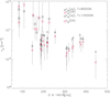 |
Fig. 10. Electron densities computed using the O IV 1399.766 Å over 1401.163 Å line ratio compared with ne(op) computed in Fig. 9. Black triangles show ne(op) computed for T = 80 000 K and black squares show ne(op) computed for T = 125 000 K. The red triangles and squares are the corresponding measurements from the O IV lines. |
Using the same procedure, we measured O IV electron densities corresponding to roughly 80 of the 443 Si IV diffusion profiles. We compared the O IV electron densities with the Si IV electron densities computed in Sect. 3.2 (Fig. 7c). We found around 20 measured ne(o4) electron densities for which the relative error Δne/ne, defined as in Eq. (12) where we replaced ne(op) with the diffusion measurement of ne, is also smaller than 0.6. The ne(o4) electron densities were found to be lower than the “diffusion” electron densities, calculated with the Si IV profiles ones, by factors in the range of 0.3–0.9. Moreover, the electron densities are found to increase as a function of the O IV 1401 Å intensity in contrast with what is found for the ne(op) cases. These results need to be confirmed with the analysis of a larger data sample.
3.5. Differentially shaped profiles
In this section we describe the analysis of differentially shaped profiles. As was described in the introduction, these profiles are composed of two or more spectral components, and present a different spectral shape for the two Si IV lines. These profiles are described with multiple Gaussian fits. In each such profile, the variation of the spectral shape is parametrized with the two or three 1393/1402 intensity ratios provided from the respective Gaussian functions. In order to track such profiles, except for the basic selection rules that were described in Sects. 2 and 3.2, we added more selection constraints for this case. We analysed individual profiles with line widths larger than the common width value, which is close to 2.7 spectral pixels for both Si IV lines. A high line width may mean that the profile includes two or even three spectral components so it could be differentially shaped. Moreover, we checked if the line ratio r = I13/I12 is either higher or lower than 2.
Finally, we kept and analysed 15 individual spectral profiles where we used simultaneously four Gaussian functions, two for the Si IV 1393.757 Å and two for the 1402.772 Å for the fit procedure. Moreover, we computed the ratio of the Gaussian intensities of the Si IV 1393.757 Å profile over the corresponding Gaussian intensities of the Si IV 1402.772 Å profile to quantify how different the shapes of the two profiles are.
In Fig. 2a the positions of multiple profiles are indicated with squares. Some multiple profiles are found along bright loop features, such as the small loop located at (697″, 329″) and one more small loop at (749″, 279″). Other profiles are at the edge of the FOV at (748″, 238″) and (749″, 236″) located at the footpoints of some loop-like features.
In Fig. 11 we show three such individual profiles of the Si IV 1393.757 Å and 1402.772 Å lines. The first column of panels shows the Si IV 1393.757 Å profiles, while the second column shows the Si IV 1402.772 Å profiles, always recorded at the same time and spatial pixel as the corresponding Si IV 1393.757 Å on the left. In all panels, the vertical dashed line indicates the zero Doppler shift position.
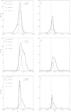 |
Fig. 11. Individual spectra of Si IV 1393.757 Å and 1402.772 Å profiles with two spectral components. First column of panels: Si IV 1393.757 Å profiles; second column: Si IV 1402.772 Å profiles. The histogram line shows the data and continuous lines show the double Gaussian fit and also the two Gaussian components forming the fit of each profile. The y-axis is in counts and the x-axis in Angstroms. The vertical dashed line shows the rest position of the Si IV lines. In the first column, each panel shows the intensity ratio r1, r2, and the ξ1, ξ2 from the corresponding Gaussian components. |
In Fig. 11, the fit of the profiles of panels a and b (749″, 279″) is composed of a wide, low-intensity Gaussian and a narrow high-intensity one. This is also the case for at least five more individual profiles in our dataset. In most cases, the wide component is redshifted relative to the narrow one. The Doppler difference for these profiles varies from 10 to 50 km s−1. These individual profiles are located close to the west border of the image (x > 720″) except one, located at (643″, 245″).
In a few cases, like in panels a and b the wide function has a ratio larger than 2 while the narrow function a ratio smaller than 2, clearly implying important differences between the two line profiles. These profiles constitute a combination of the previous cases examined in Sects. 3.2 and 3.3 because some components can be dominated by opacity while other components can be dominated by resonant scattering.
We computed the non-thermal velocities ξ of the narrow and wide functions, using a spectral point spread function FWHM of 0.02585 Å (De Pontieu et al. 2014). For this calculation we used a temperature of 40000 K for the maximum concentration of the Si IV ions (Avrett et al. 2013). The narrow Gaussian components can have values from 4.4 up to 10 km s−1. Such narrow profiles have being identified with IRIS in other cases (Hou et al. 2016).
The Si IV spectral profiles, with many Doppler components, have been found along cool loops with IRIS, either at their footpoints or along their length (Huang et al. 2015). In our study, we have some profiles located along loops. The different spectral components have different Doppler shifts and indicate plasma volumes moving with different velocities. This suggests that they belong to different loop strands and that there the plasma is affected by resonant scattering or opacity at various degrees.
Finally, we confirm with the Si IV profiles the SUMER result obtained in the C IV 1548.189 Å and 1550.775 Å lines (see Gontikakis & Vial 2016): in some regions the two lines of the respective doublets show, a noticeable differential behaviour.
4. Discussion and conclusion
This work analyses cases where the emission profiles of Si IV 1393.757 Å and 1402.772 Å cannot be described only by optically thin emission caused by electron collisional excitations.
We studied individual profiles with line ratios 1393.757/1402.772 larger than 2, where the resonant scattering was dominant. We found roughly 4000 such profiles that represent more than 2% of the raster individual profiles for which we could compute a Gaussian fit. The high value of the line ratio does not seem to be caused by a local high incident radiation, such as a bright point, but rather by a decrease of the collision term in the line formation. This is a conclusion which is consistent with our finding with the SUMER data (Gontikakis & Vial 2016).
We derived electron densities with values decreasing by roughly an order of magnitude when the line ratios rise from 2.1 to 2.5 (Fig. 7c). The calculated electron densities depend on the temperature and on the supposed altitude of the structure and can range from 2 × 10⁹ up to 5 × 1011 cm−3.
A second class of profiles are the ones with a line ratio lower than 2. In these cases the radiation is influenced by opacity. We found roughly 500 cases with low line ratios. This represents a small fraction of the profiles influenced by opacity as we took into account only profiles for which the lines ratio is lower than 1.6. These profiles are formed in structures surrounding quiet Sun areas as seen in Fig. 2a. To compute the optical depth, we assumed a constant source function along the structure, and we found values between 1.6 and 3 for most cases. Some of these points belong to an elongated fibril 3–4″ in length. Only a small fraction of these structures is actually optically thick.
We measured electron densities ne(o4) from the O IV line ratio 1399.766/1401.163 profiles, selected at the same spatial locations where the Si IV ones presented diffusion or opacity effects. The ne(o4) and ne(op) cases where we found similar values are found to decrease as a function of O IV 1401.163 Å intensity (Fig. 10). The values of ne(o4) and ne derived at diffusion regions show an opposite dependence on O IV 1401.163 Å intensity but better statistics are required to confirm this result. A more thorough approach taking into account the filling factors should be undertaken in a future project.
A possible cause of the high opacity is that these profiles emerge from elongated structures, oriented along the LOS. Most of these structures connect the active region positive magnetic field with the neighbouring faint field. They could correspond to fibrils, seen in Hα. Their calculated electron densities can vary from 109 cm−3 to a few times 1011 cm−3 depending on the supposed plasma temperature and under the assumption of ionization equilibrium.
We also found examples where the spectral shape of the Si IV 1393.757 Å profile is different from the spectral shape of the Si IV 1402.772 Å one. Such cases can be explained by a combination of differential motions along the LOS at the sub-spatial resolution scale, concerning plasma volumes that are affected by resonant scattering, at different degrees.
In some cases, the intensity ratio of one of the Gaussian components was higher than 2, showing resonant scattering, while the ratio of the second Gaussian was smaller than 2 showing that opacity is dominant there. Such are the cases of Fig. 11. In these cases, the mechanisms of high opacity and resonant scattering, co-exist in the same profiles and must originate from independent plasma volumes.
This effect of differential profiles was also analysed using the C IV 1548.189 Å and 1550.775 Å lines observed with SUMER (Gontikakis & Vial 2016). In the case of the Si IV profiles, the phenomenon is less common than in the case of the C IV profiles. However, it is one more proof that such profiles can be observed on the Sun. Moreover, in the case of IRIS observations these profiles are not affected by polarization as might be the case for the SUMER observed profiles.
As previously mentioned, we have searched for a spatial signature of the three types of outlier profiles (see Fig. 2a). At the suggestion of De Pontieu (2017, priv. comm.), we built a movie from the Si IV slit-jaw images where the occurrence of these profiles appears at their temporal and spatial positions on the slit (online; the profiles’ convention is the same as in Fig. 2a). In the movie we notice the same concentration of diffusion and opacity profiles surrounding the quiet Sun areas as in Fig. 2a.
In summary we studied three categories of profiles that are represented by a number of examples. The first category includes roughly 4000 cases with a line ratio higher than 2, the second category includes roughly 500 optically thick profiles. Finally there is the category of the 15 multi-component profiles.
However, we were obliged to exclude many candidate profiles from our study because of poor statistics. It is possible that such resonance or/and opacity dominated profiles, form a more important fraction of the IRIS Si IV raster images.
Consequently, as far as the plasma diagnostic from spectral lines is concerned, one needs to have in mind that collisional processes are not the sole mechanism in the transition region, for the diagnostic of spectral profiles.
In order to obtain a larger statistical basis, we believe that such a study should be repeated with other IRIS data. Moreover, a future spectrograph with an increased sensitivity would allow to analyse more cases that had to be excluded in our study because the profiles were too noisy.
Movies
Movie of Fig. 3 Access here
Acknowledgments
We would like to thank the anonymous referee for his or her very useful comments. CG would like to thank the Université Paris-Sud which made possible his visit at the Institut d’Astrophysique Spatiale during April 2017. He would also like to thank ESA for funding his participation in the IRIS-9 workshop held in Göttingen. We would like to thank Bart De Pontieu for his critical comments and suggestions and Wei Liu, Jean-Pierre Wuelser and the team of the IRIS spectrograph at LMSAL for useful comments on the data. CHIANTI is a collaborative project including George Mason University, the University of Michigan (USA), and the University of Cambridge (UK). The authors gratefully acknowledge use of data from the IRIS and SDO (AIA and HMI) databases. IRIS is a NASA small explorer mission developed and operated by LMSAL with mission operations executed at NASA Ames Research Centre and major contributions to downlink communications funded by ESA and the Norwegian Space Centre.
References
- Avrett, E., Landi, E., & McKillop, S. 2013, ApJ, 779, 155 [NASA ADS] [CrossRef] [Google Scholar]
- Buchlin, E., & Vial, J.-C. 2009, A&A, 503, 559 [NASA ADS] [CrossRef] [EDP Sciences] [Google Scholar]
- Chambe, G., & Henoux, J.-C. 1979, A&A, 80, 123 [NASA ADS] [Google Scholar]
- Del Zanna, G., Dere, K. P., Young, P. R., Landi, E., & Mason, H. E. 2015, A&A, 582, A56 [NASA ADS] [CrossRef] [EDP Sciences] [Google Scholar]
- De Pontieu, B., Title, A. M., Lemen, J. R., et al. 2014, Sol. Phys., 289, 2733 [NASA ADS] [CrossRef] [Google Scholar]
- Dere, K. P., & Mason, H. E. 1993, Sol. Phys., 144, 217 [NASA ADS] [CrossRef] [Google Scholar]
- Dere, K. P., Landi, E., Mason, H. E., Monsignori Fossi, B. C., & Young, P. R. 1997, A&AS, 125, 149 [NASA ADS] [CrossRef] [EDP Sciences] [Google Scholar]
- de Wijn, A. G., & De Pontieu, B. 2006, A&A, 460, 309 [NASA ADS] [CrossRef] [EDP Sciences] [Google Scholar]
- Dudík, J., Del Zanna, G., Dzifčáková, E., Mason, H. E., & Golub, L. 2014, ApJ, 780, L12 [NASA ADS] [CrossRef] [Google Scholar]
- Dumont, S., Pecker, J.-C., Mouradian, Z., Vial, J.-C., & Chipman, E. 1983, Sol. Phys., 83, 27 [CrossRef] [Google Scholar]
- Fischbacher, G. A., Loch, S. D., & Summers, H. P. 2002, A&A, 389, 295 [NASA ADS] [CrossRef] [EDP Sciences] [Google Scholar]
- Gontikakis, C., & Vial, J.-C. 2016, A&A, 590, A86 [NASA ADS] [CrossRef] [EDP Sciences] [Google Scholar]
- Gontikakis, C., Winebarger, A. R., & Patsourakos, S. 2013, A&A, 550, A16 [NASA ADS] [CrossRef] [EDP Sciences] [Google Scholar]
- Guglielmino, S. L., Zuccarello, F., Young, P. R., Murabito, M., & Romano, P. 2018, ApJ, 856, 127 [NASA ADS] [CrossRef] [Google Scholar]
- Hassler, D. M., Lemaire, P., & Longval, Y. 1997, Appl. Opt., 36, 353 [NASA ADS] [CrossRef] [Google Scholar]
- Heinzel, P. 2015, Astrophys. Space Sci. Lib., 415, 103 [NASA ADS] [CrossRef] [Google Scholar]
- Hou, Z., Huang, Z., Xia, L., et al. 2016, ApJ, 829, L30 [NASA ADS] [CrossRef] [Google Scholar]
- Huang, Z., Xia, L., Li, B., & Madjarska, M. S. 2015, ApJ, 810, 46 [NASA ADS] [CrossRef] [Google Scholar]
- Jejčič, S., & Heinzel, P. 2009, Sol. Phys., 254, 89 [NASA ADS] [CrossRef] [Google Scholar]
- Jejčič, S., Susino, R., Heinzel, P., et al. 2017, A&A, 607, A80 [NASA ADS] [CrossRef] [EDP Sciences] [Google Scholar]
- Jordan, C., Bartoe, J.-D. F., Brueckner, G. E., et al. 1979, MNRAS, 187, 473 [NASA ADS] [Google Scholar]
- Judge, P. G., & Pietarila, A. 2004, ApJ, 606, 1258 [NASA ADS] [CrossRef] [Google Scholar]
- Landi, E., Del Zanna, G., Young, P. R., Dere, K. P., & Mason, H. E. 2012, ApJ, 744, 99 [NASA ADS] [CrossRef] [Google Scholar]
- Lites, B. W., & Cook, J. W. 1979, ApJ, 228, 598 [NASA ADS] [CrossRef] [Google Scholar]
- Lites, B. W., Hansen, E. R., & Shine, R. A. 1980, ApJ, 236, 280 [NASA ADS] [CrossRef] [Google Scholar]
- Mariska, J.T. 1992, The solar transition region (Cambridge, NY: Cambridge University Press) [Google Scholar]
- Mason, H. E., & Monsignori Fossi, B. C. M. 1994, A&ARv, 6, 123 [NASA ADS] [CrossRef] [Google Scholar]
- Pesnell, W. D., Thompson, B. J., & Chamberlin, P. C. 2012, Sol. Phys., 275, 3 [NASA ADS] [CrossRef] [Google Scholar]
- Scherrer, P. H., Schou, J., Bush, R. I., et al. 2012, Sol. Phys., 275, 207 [Google Scholar]
- Schmit, D. J., Innes, D., Ayres, T., et al. 2014, A&A, 569, L7 [NASA ADS] [CrossRef] [EDP Sciences] [Google Scholar]
- Seaton, M. J. 1964, Planet. Space Sci., 12, 55 [NASA ADS] [CrossRef] [Google Scholar]
- Skogsrud, H., Rouppe van der Voort, L., & De Pontieu, B. 2016, ApJ, 817, 124 [NASA ADS] [CrossRef] [Google Scholar]
- Teriaca, L., Banerjee, D., & Doyle, J. G. 1999, A&A, 349, 636 [NASA ADS] [Google Scholar]
- Tsiropoula, G., Tziotziou, K., Kontogiannis, I., et al. 2012, Space Sci. Rev., 169, 181 [NASA ADS] [CrossRef] [Google Scholar]
- Wilhelm, K., Curdt, W., Marsch, E., et al. 1995, Sol. Phys., 162, 189 [NASA ADS] [CrossRef] [Google Scholar]
- Yan, L., Peter, H., He, J., et al. 2015, ApJ, 811, 48 [NASA ADS] [CrossRef] [Google Scholar]
- Young, P. R. 2015, ArXiv e-prints [arXiv:1509.05011] [Google Scholar]
- Zirin, H. 1988, Astrophysics of the Sun (Cambridge, NY: Cambridge University Press) [Google Scholar]
All Figures
|
Fig. 1. Temporal evolution of C IV 1548.189 Å and 1550.775 Å line profiles during a flare, observed in August 1973 with S082B spectrograph on Skylab, (Fig. 1c from Lites & Cook 1979, p. 599, © AAS. Reproduced with permission). |
| In the text | |
|
Fig. 2. Panel a: raster intensity image of the Si IV 1393.757 Å line. High 1393/1402 ratios are indicated with red triangles, blue diamonds indicate low line ratios, and green squares indicate differentially shaped profiles. Panel b: raster-like HMI/SDO magnetogram of the same region. |
| In the text | |
|
Fig. 3. Slit jaw image in the 1400 Å passband. Triangles, diamonds, and squares have the same meaning as in Fig. 2a. The positions indicated with these symbols correspond to spectral profiles recorded during the raster between 01:35:44 UT and 01:36:21 UT. Ninety-eight of these slit jaw images form a movie (available online). |
| In the text | |
|
Fig. 4. Panel a: map of I13/I12 line ratio. The colours range from 1.6 to 2.3. The map is smoothed to 3 × 3 pixels. Black areas do not have a signal because their counts are too low. The white isocontours indicate the 1.9 values and the black isocontours the 2.1 ratios. Panel b: scatter plot of line ratio as a function of I13, the Si IV 1393.757 Å intensity. The black and blue plus signs represent the selected points with line ratios higher than 2. Black plus signs also indicate selected points with line ratios lower than 1.6 |
| In the text | |
|
Fig. 5. Eight selected profiles of the Si IV 1393.757 Å (thin histogram line) and 1402.772 Å (thick histogram line) spectral lines where the lines ratio (r) is higher than 2. The data are represented with a histogram line while the Gaussian fit with a continuous line. The horizontal axis is in spectral pixels and the vertical axis in Data numbers. The dashed vertical shows the rest position for both lines. In each panel we show the total intensities line ratio. |
| In the text | |
|
Fig. 6. Geometry of the incident radiation. A point S is at a distance h above the solar surface. The segment SC, where C is the solar centre, meets the surface at P(xD,yD). The point B is at the largest distance from where photons can reach S. The projected distance on the image is Dmax and θmax the angle at S. The point A(x,y) represents an intermediate position from where light can reach S , and γ is the angle between SA and the normal to the solar surface. |
| In the text | |
|
Fig. 7. Panel a: |
| In the text | |
|
Fig. 8. Eight selected profiles of the Si IV 1393.757 Å and 1402.772 Å lines where the lines ratio is lower than 1.6. The data and the fit are represented as in Fig. 11. In each panel we show the total intensity line ratio (r) and the position of the profiles on Fig. 2a. The axes definitions are as in Fig. 5. |
| In the text | |
|
Fig. 9. Panel a: electron densities as a function of the structure width, calculated for three ionization equilibrium temperatures 50 000 K (plus signs), 80 000 K, (triangles) and 125000 K (squares). Panel b: opacity, computed using Eq. (10), as a function of the width. |
| In the text | |
|
Fig. 10. Electron densities computed using the O IV 1399.766 Å over 1401.163 Å line ratio compared with ne(op) computed in Fig. 9. Black triangles show ne(op) computed for T = 80 000 K and black squares show ne(op) computed for T = 125 000 K. The red triangles and squares are the corresponding measurements from the O IV lines. |
| In the text | |
|
Fig. 11. Individual spectra of Si IV 1393.757 Å and 1402.772 Å profiles with two spectral components. First column of panels: Si IV 1393.757 Å profiles; second column: Si IV 1402.772 Å profiles. The histogram line shows the data and continuous lines show the double Gaussian fit and also the two Gaussian components forming the fit of each profile. The y-axis is in counts and the x-axis in Angstroms. The vertical dashed line shows the rest position of the Si IV lines. In the first column, each panel shows the intensity ratio r1, r2, and the ξ1, ξ2 from the corresponding Gaussian components. |
| In the text | |
Current usage metrics show cumulative count of Article Views (full-text article views including HTML views, PDF and ePub downloads, according to the available data) and Abstracts Views on Vision4Press platform.
Data correspond to usage on the plateform after 2015. The current usage metrics is available 48-96 hours after online publication and is updated daily on week days.
Initial download of the metrics may take a while.