| Issue |
A&A
Volume 619, November 2018
|
|
|---|---|---|
| Article Number | A100 | |
| Number of page(s) | 10 | |
| Section | The Sun | |
| DOI | https://doi.org/10.1051/0004-6361/201732530 | |
| Published online | 15 November 2018 | |
Eruption of a multi-flux-rope system in solar active region 12673 leading to the two largest flares in Solar Cycle 24⋆
1
CAS Key Laboratory of Solar Activity, National Astronomical Observatories, Chinese Academy of Sciences, 100101 Stavropol, PR China
e-mail: This email address is being protected from spambots. You need JavaScript enabled to view it.
; This email address is being protected from spambots. You need JavaScript enabled to view it.
2
School of Astronomy and Space Science, University of Chinese Academy of Sciences, 100049 Beijing, PR China
Received:
22
December
2017
Accepted:
21
August
2018
Abstract
Context. Solar active region (AR) 12673 in 2017 September produced the two largest flares in Solar Cycle 24: the X9.3 flare on September 6 and the X8.2 flare on September 10.
Aims. We attempt to investigate the evolutions of the two large flares and their associated complex magnetic system in detail.
Methods. Combining observations from the Solar Dynamics Observatory and results of nonlinear force-free field (NLFFF) modeling, we identify various magnetic structures in the AR core region and examine the evolution of these structures during the flares.
Results. Aided by the NLFFF modeling, we identify a double-decker flux rope configuration above the polarity inversion line (PIL) in the AR core region. The north ends of these two flux ropes were rooted in a negative- polarity magnetic patch, which began to move along the PIL and rotate anticlockwise before the X9.3 flare on September 6. The strong shearing motion and rotation contributed to the destabilization of the two magnetic flux ropes, of which the upper one subsequently erupted upward due to the kink-instability. Then another two sets of twisted loop bundles beside these ropes were disturbed and successively erupted within five minutes like a chain reaction. Similarly, multiple ejecta components were detected as consecutively erupting during the X8.2 flare occurring in the same AR on September 10. We examine the evolution of the AR magnetic fields from September 3 to 6 and find that five dipoles emerged successively at the east of the main sunspot. The interactions between these dipoles took place continuously, accompanied by magnetic flux cancellations and strong shearing motions.
Conclusions. In AR 12673, significant flux emergence and successive interactions between the different emerging dipoles resulted in a complex magnetic system, accompanied by the formations of multiple flux ropes and twisted loop bundles. We propose that the eruptions of a multi-flux-rope system resulted in the two largest flares in Solar Cycle 24.
Key words: sunspots / Sun: activity / Sun: atmosphere / Sun: flares / Sun: magnetic fields
The movies associated to Figs. 3–5, 7, 8 are available at https://www.aanda.org
© ESO 2018
1. Introduction
Solar flares are explosive phenomena on the Sun that can be observed from X-ray to radio wavelengths, and that release dramatic free magnetic energy stored in the solar atmosphere via the process of magnetic reconnection (Priest & Forbes 2002; Schmieder et al. 2015). In previous studies, the accumulation of free magnetic energy in the solar atmosphere is demonstrated to be mainly caused by three types of mechanisms: (1) magnetic flux emergence or cancellation (Wang & Shi 1993; Chen & Shibata 2000, Zhang et al. 2001; Sterling et al. 2010; Louis et al. 2015), (2) shearing motion (Wang et al. 1994; Meunier & Kosovichev 2003; Sun et al. 2012), (3) sunspot rotation (Brown et al. 2003; Zhang et al. 2007; Török et al. 2013). Although the energy accumulation has been investigated thoroughly, it is difficult for us to comprehend the detailed process of violent energy release in various solar eruptions. Because it is widely accepted that magnetic flux ropes play key roles in triggering eruptive events (Amari et al. 2000; Fan 2005; Kliem et al. 2010; Liu et al. 2010; Green et al. 2011; Li et al. 2016; Yan et al. 2017), we can understand these eruptive events such as solar flares and coronal mass ejections (CMEs) through studying magnetic flux ropes.
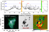 |
Fig. 1. Flares produced by AR 12673. Panel a: GOES SXR 1–8 Å flux variation from 2017 September 3 to September 11. Four X-class flares took place during this period, of which the two largest ones reached up to X9.3 (orange region) and X8.2 (green region), respectively. The blue horizontal dotted lines mark the threshold levels of M1.0 and X1.0 flares. Panels b–d: overview of the X9.3 flare in AR 12673 on September 6. The AIA 94 Å image in panel b shows this AR at the onset of the flare. HMI continuum intensitygram and LOS magnetogram in panels c and d display the sunspots and underlying magnetic fields in the AR core region, whose field of view (FOV) is outlined by the green square in panel b. |
A magnetic flux rope is a set of magnetic field lines winding around a central axis in classical eruptive flare models and many CME observations. A huge amount of effort has been made in numerical simulations of the formation and dynamic activity of flux ropes (Forbes & Priest 1995; Aulanier et al. 2010). Amari et al. (2000, 2003) simulated the evolution of a flux rope and proposed that a slow converging motion of the footpoints of field lines toward the polarity inversion line (PIL) contributed to the formation of a flux rope through magnetic reconnection. With high-resolution observations, the existence of flux ropes in the solar atmosphere has also been recently evidenced (Guo et al. 2010, 2013; Cheng et al. 2011; Yang et al. 2014; Kumar et al. 2017, Guglielmino et al. 2017; Wang et al. 2017a; Yan et al. 2018a; Shen et al. 2018b). Zhang et al. (2012) reported a flux rope observed as a hot extreme ultraviolet (EUV) channel before and during the solar eruption and proposed that the instability of this flux rope triggered the eruption. Li & Zhang (2013a) investigated the successive eruptions of two flux ropes during an M-class flare. Li & Zhang (2013b) presented four homologous flux ropes, which were formed successively at the same location in an active region (AR). These observations imply that flux ropes may be ubiquitous on the Sun (Zhang et al. 2015; Hou et al. 2016). In the present work, a magnetic flux rope is defined as a set of magnetic field lines winding around a central axis by more than one full turn (Liu et al. 2016). Then aided by nonlinear force-free field (NLFFF) modeling and the calculation of twist number, we can identify a magnetic flux rope without ambiguity.
Flux ropes are often related to various magnetohydrodynamic (MHD) instability processes, which eventually trigger solar flares and CMEs (Alexander et al. 2006; Liu et al. 2007; Kumar & Cho 2014). Kink MHD instability is triggered by the azimuthal twist of magnetic tubes. Numerical simulations of the kink instability suggest that if the twist of a flux rope exceeds a critical value, then this rope becomes unstable (Kliem et al. 2004). The exact value of required twist depends on various factors such as loop geometry and overlying magnetic fields (Hood & Priest 1979; Baty 2001; Fan & Gibson 2004; Leka et al. 2005). In addition, observations of kink instability were reported recently by many authors (Srivastava et al. 2010; Wang et al. 2017b).
From 2017 September 4 to September 10, AR 12673 produced a total of 4 X-class flares, 27 M-class flares, and a multitude of smaller ones (see the details in Yang et al. 2017). The X9.3 flare on September 6 is the largest flare in Solar Cycle 24 and has been reported in several works (Wang et al. 2018; Verma 2018; Shen et al. 2018a; Yan et al. 2018b; Jiang et al. 2018). In this work, we identify a double-decker flux rope configuration above the PIL in the AR core region and detect successive eruptions of multiple flux ropes and twisted loop bundles within five minutes before the peak of this large flare. A similar phenomenon was also observed during the X8.2 flare on September 10. Here we investigate the evolutions of the two large flares and the associated complex magnetic system in detail.
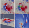 |
Fig. 2. Double-decker flux rope configuration above the PIL in the AR core region revealed by NLFFF modeling at 11:24 UT on 2017 September 6. Panels a–b: top view and side view of two flux ropes (FR1 and FR2) composing the double-decker configuration. The FOV of these panels is approximated by the white square in Fig. 1d. Panel c: isosurfaces of twist number Tw = –1 (white) and Tw = –1.75 (red) viewed from the same perspective as panel a. Panel d: twist number distribution in the vertical (x–z) plane along the green cut labeled in panel c. |
The remainder of this paper is structured as follows. Section 2 contains the observations and data analysis taken in our study. The detailed process of the two flares and the evolution of the magnetic fields in the AR core region are presented in Sect. 3. Finally, in Sect. 4 we conclude this work and discuss the results.
2. Observations and data analysis
On 2017 September 6, an X9.3 flare took place in NOAA AR 12673, which was the largest flare in Solar Cycle 24. About four days later, another X8.2 flare happened in the same AR when the AR rotated to the solar southwestern limb on September 10. The Atmospheric Imaging Assembly (AIA; Lemen et al. 2012) on board the Solar Dynamics Observatory (SDO; Pesnell et al. 2012) successively observes multilayered solar atmosphere in ten (E)UV passbands with a cadence of (12)24 s and a spatial resolution of 1ʺ̣2. The SDO/Helioseismic and Magnetic Imager (HMI; Schou et al. 2012) provides one-arcsecond resolution full-disk line-of-sight (LOS) magnetograms and intensitygrams every 45 s, and photospheric vector magnetograms at a cadence of 720 s (Hoeksema et al. 2014). Here we employ the data of AIA 94 Å, 171 Å, 304 Å, HMI LOS magnetograms, intensitygrams and the HMI data product called Space-weather HMI Active Region Patches (SHARP; Bobra et al. 2014) for the investigation of the X9.3 flare on September 6. The AIA 131 Å and 171 Å images are used to study the X8.2 flare on September 10. Moreover, the observations from the Geostationary Operational Environmental Satellite (GOES) are also used to present the variation of soft X-ray (SXR) 1–8 Å flux from September 3 to September 11.
The AIA and HMI observations used in the X9.3 flare are all derotated to the reference time of 12:02 UT on September 6, and the AIA data of the X8.2 flare are aligned to 16:06 UT on September 10. To investigate the evolution of magnetic fields in AR 12673 before the onset of the X9.3 flare, we employ the HMI LOS magnetograms and intensitygrams from September 3 to September 6 and derotate them to a middle time of 00:00 UT on September 05. To determine the horizontal photospheric velocities, we apply the method of differential affine velocity estimator (DAVE; Schuck 2006). The window size in DAVE is set as 19 pixels, following the parameter given in Liu et al. (2013).
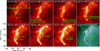 |
Fig. 3. Eruption of the double-decker flux rope configuration. Panels a1 –a7: sequence of extended AIA 304 Å images showing the filament and eruption process of the double-decker flux rope configuration. The two filaments and associated brightening before their eruption are denoted by green arrows in panels a1 –a4. The green curves in panels a6 and a7 delineate the twisted threads and the writhed structure of the upper flux rope (FR2). Panel b: corresponding 94 Å image exhibiting the double-decker flux rope configuration in a higher temperature wavelength. The FOV is outlined by the white square in Fig. 1(d). An animation (1.mpg) of the 304 Å and the 94 Å images is available online. |
In order to reconstruct the three-dimensional (3D) coronal structure in the target region, we utilize the “weighted optimization ” method to perform NLFFF extrapolation (Wiegelmann 2004; Wiegelmann et al. 2012) based on the observed photospheric vector magnetic fields. To satisfy the force-free condition, the vector magnetograms are preprocessed by a procedure developed by Wiegelmann et al. (2006) towards suitable photospheric boundary conditions. The calculation is performed within a box of 512 × 448 × 256 uniform grid points (186 × 162 × 93 Mm3), which covers nearly the entire AR. We further calculate the twist number Tw (Berger & Prior 2006) of the extrapolated field using the code developed by R. Liu and J. Chen (Liu et al. 2016).
3. Results
3.1. Overview of AR 12673
When AR 12673 approached the solar center on September 03, significant flux emergence commenced in this region and persisted for the following several days (Sun & Norton 2017). Before disappearing completely in the west solar limb on September 11, AR 12673 produced a total of 4 X-class flares, 27 M-class flares, and numerous smaller ones. Figure 1a shows the GOES SXR 1–8 Å flux variation from September 3 to September 11, and four X-class flares are denoted. The orange and green regions in panel a respectively mark the two largest flares in Solar Cycle 24: the X9.3 flare on September 6 and the X8.2 flare on September 10. In AIA 94 Å channel, the X9.3 flare performed complex structures accompanied by intense emission enhancement (panel b). This flare started around 11:53 UT and peaked at 12:02 UT when the AR was centered around S09W34. Panels c and d show the HMI continuum intensitygram and LOS magnetogram of the AR at the onset of the flare.
3.2. The X9.3 flare on September 6
Based on the photospheric vector magnetograms observed by SDO/HMI, we extrapolated the 3D structure of the AR using NLFFF modeling at 11:24 UT on September 6, just before the occurrence of the X9.3 flare. For visualizations of the magnetic field above the region of interest, we select a region from the NLFFF extrapolation, with an FOV approximated by the white box in Fig. 1d, to display in Fig. 2. Moreover, we calculate the twist number Tw of the reconstructed field and then we can obtain the photospheric twist map or vertical twist map in the selected cutting plane. According to the photospheric twist map and the definition of magnetic flux rope mentioned in Sect. 1, we plot the field lines across the photosphere where the ∣Tw∣ ≧ 1.0 near the PIL in the AR core region. As a result, we obtain two magnetic flux ropes with Tw ≦ –1.0, of which the upper one (FR2) is located right above the lower one (FR1), forming a double-decker flux rope configuration (Liu et al. 2012). Figures 2a and b show the top view and side view of the double-decker flux rope configuration, respectively. The background is the photospheric vertical magnetic field (Bz). Panel (c) exhibits the isosurfaces of Tw = –1 (white) and Tw = –1.75 (red) above the PIL from the top view. It is clear that the isosurface of Tw = –1 roughly outlines the two flux ropes and the ∣Tw∣ around the axes of the two flux ropes is beyond 1.75. Along the green cut marked in panel c, we make a twist map in the vertical (x –z) plane and show it in panel d. One can see that there are two regions with high negative twist number in this vertical twist map, which correspond to the cross sections of the two flux ropes.
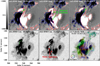 |
Fig. 4. Magnetic evolution of the AR core region during the X9.3 flare. Panels a1 –a3: HMI LOS magnetograms with contours of ± 400 G displaying the magnetic fields of the core region before and after the flare peak at 12:02 UT. The green solid arrows in panels a1 and a3 denote the direction of rapid displacement of the negative patch where the north ends of the double-decker flux rope configuration are rooted. The green arrows in panel a2 mark the magnetic transients caused by the white-light flare. Panels b1–b2: corresponding HMI continuum intensitygrams. The green arrow in panel b1 labels the rotation of the negative patch. The red arrows in panel b2 mark the signals of the white-light flare. Panel c: the horizontal photospheric velocity field (colored arrows) derived from the HMI continuum intensitygrams computed by the DAVE method. In the lower-left corner, the radius of the circle corresponds to a speed of 0.3 km s−1, and the color of an arrow corresponds to its direction. The FOV is the same as Fig. 3. An animation (2.mpg) of the HMI continuum intensitygrams and LOS magnetograms is available online. |
By examining the AIA 304 Å observations, we detected two sets of filament threads located in the AR core region before the occurrence of the X9.3 flare (see F1 and F2 in Fig. 3a1 and the corresponding animation). According to Fig. 2, we suggest that F1 corresponds to the upper flux rope FR1 and F2 corresponds to the lower rope FR2. Around 11:53:53 UT, brightening appeared at the north cross site of these two filament threads (flux ropes) and continued for several minutes, implying the interaction between rising FR1 and FR2. Then south ends of FR2 and FR1 brightened in tandem at 11:54:41 UT and 11:54:29 UT, respectively (Fig. 3a2–a3). At 11:54:41 UT, brightening at the south cross site of FR1 and FR2 was detected as well. The two flux ropes then were tracked completely by the brightening material, and FR2 began to moved upward as well (see panel a5). In panel a6, we can see that FR2 showed obvious twisted threads while FR1 had erupted outwards. At 11:56:08 UT, the writhed structure of FR2 appeared (see panel a7). As shown in Fig. 2c, at 11:24 UT, the maximum ∣Tw∣ of FR2 was beyond 1.75, which is the threshold value of kink instability (Török et al. 2004). Combined with the observations of writhed structure, the high Tw of FR2 implied the occurrence of kink instability. In 94 Å channel, the two flux ropes were also observed clearly at 11:55:23 UT (panel b).
Through checking the HMI data, we notice that the double-decker flux rope configuration was lying above a semicircular PIL (see Fig. 4). It is shown that the south ends of the two flux ropes were rooted in positive magnetic fields to the southwest of the PIL, and their north ends in a negative-polarity patch to the northeast of the PIL. Before the onset of the X9.3 flare, this negative magnetic patch kept moving northwestward along the semicircular PIL and successively sheared with the adjacent positive fields (see panels a1–a3 and the corresponding animation). Meanwhile, the HMI continuum intensitygrams reveal that this negative patch exhibited a counterclockwise rotation motion (panel b1). The shearing motion and rotation of this negative magnetic patch can be seen clearly in the velocity map of panel c. As a result, the twist number of the two flux ropes rooted in this negative patch could gradually increase, and eventually approach or exceed the threshold value of kink instability, leading to the onset of this large flare. Furthermore, when the flare occurred, a white-light flare can be identified in the HMI continuum intensitygram (panel b2), and the LOS magnetogram exhibited magnetic transients as well (panel a2).
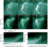 |
Fig. 5. Dynamic evolutions of the complex system consisting of multiple flux ropes and twisted loop bundles during the X9.3 flare. Panels a1 –a3: sequence of AIA 94 Å images showing the interaction between FR2 and the first twisted loop bundles (LB1). The red curves delineate their main axes. The white solid arrows in panel a1 mark the rising directions of FR2. The white arrows in panels a2–a3 denote the moving direction of LB1 after the interaction with FR2. Panels b1–b3: 94 Å images with a larger FOV exhibiting LB1 and the second twisted loop bundles (LB2). The green square in panel b2 outlines the FOV of panels a1– a3. Panels d1–d2: time-space plots along arc-sector domains “A–B” of panel b1 and “C–D” of panel b3 in 94 Å channel. The red lines approximate trajectories of FR2, LB1, and LB2. The full temporal evolution of the 94 Å images is available as an online movie (3.mpg). |
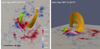 |
Fig. 6. Extrapolated 3D NLFFF structures corresponding to FR1, FR2, LB1, and LB2 at 11:24 UT on 2017 September 6. Panel a: shows these structures from a top view, and panel b shows them from a side view. The FOV of this figure is similar to that of Figs. 1c–d. |
During the X9.3 flare, we identify a total of two flux ropes and some twisted loop bundles in the flaring region (see Fig. 5 and the corresponding animation). In 94 Å images of panels a1–a3, we show the interaction between the kink-unstable FR2 described in Figs. 2 and 3, and the nearby loop bundles (LB1). They are outlined respectively with red dotted and dashed curves. At 11:55:23 UT, FR2 was rising in the northwest direction, approaching the adjacent LB1. Around 11:56:23 UT, FR2 and LB1 interacted with each other in their middle parts (panel a2). Then LB1 began to rise up rapidly (panel a3). In panels b1–b3, we show LB1 and another set of loop bundles (LB2) with a larger scale. The green arc-sector domain “A–B” in panel b1 is approximately along the erupting directions of FR2 and LB1, and the domain “C–D” in panel b3 is in the direction of LB2. Along the two arc-sector domains, we make two time-space plots and show them in panels d1 and d2, respectively. Panel d1 shows that FR2 began to rise upward at about 11:55:30 UT, accompanied by the brightening at its base. Around 11:57:30 UT, FR2 approached LB1 with a projected velocity of ∼280 km s−1, and then FR2 started to erupt with a speed of ∼380 km s−1. As shown in panel d2, LB2 was disturbed around 12:00 UT and then erupted with a projected velocity of ∼200 km s−1. After the successive eruptions of multiple flux ropes and twisted loop bundles, the X9.3 flare reached its peak at 12:02 UT.
In order to verify these structures illuminated in EUV channels and study their magnetic topologies, we reconstruct 3D magnetic field above the AR and select a larger FOV involving all the structures mentioned above to show in Fig. 6. Similar to the analysis of Fig. 2, after calculating the Tw of the reconstructed field, we plot the field lines across the photosphere where the ∣Tw∣ ≧ 1.0 near the PIL in the AR core region and then get two magnetic flux ropes: the pink FR1 and the red FR2. Resetting the filter value of ∣Tw ∣ as 0.5, we obtain a set of green twisted loop bundles beside the FR2, which corresponds to the LB1. Around the main sunspot, we track the field lines and get another set of orange loop bundles (LB2) with a smaller ∣Tw∣. Panels a and b exhibit these structures from the top view and side view, respectively. It is worthy noting that, due to the projection effect, these structures located in the southwest region of the solar surface would present different shapes in the remotely-sensed images compared with that seen from the top view in the reconstructed field by NLFFF modeling.
3.3. The formation and evolution of the complex magnetic fields of AR 12673
Successive eruptions of multiple flux ropes and twisted loop bundles during the X9.3 flare implies the existence of a complex magnetic system in the AR core region. To investigate the formation and evolution of such a complicated magnetic system, we analyze the HMI observations in AR 12673 (see Fig. 7 and the corresponding animation). At the initial stage of the AR evolution, there was simply one main sunspot with positive polarity in the AR center. Then on September 3, one pair of dipolar fields emerged to the southeast of the main sunspot (see the “Dipole 1” in Fig. 5a), followed by the emergence of another dipolar region to the northeast of the main sunspot (see the “Dipole 2” in panel b). After this, the negative and positive patches of “Dipole 1” separated in the east-west direction, as well as the patches of “Dipole 2”. Due to the existence of the main sunspot with strong fields, the positive patches of these two dipoles were blocked (Yang et al. 2017). Thus, an elongated positive region was formed on the east side of the main sunspot (see panel b). Between the negative and positive patches of these two dipoles, a semicircular channel was formed. Then on September 4, two pairs of dipolar fields newly emerged within this semicircular channel (see the “Dipole 3” and “Dipole 4” in panel c), and their patches with opposite polarities separated along the north-south axis of the channel. Here we speculate that magnetic reconnection took place between “Dipole 1” and “Dipole 4”, forming the FR1 and FR2 whose north ends were rooted in the negative patch of “Dipole 4” and south ends rooted in the positive patch of “Dipole 1”. A similar process could have occurred between “Dipole 2” and “Dipole 3” and formed LB2.
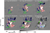 |
Fig. 7. Sequence of HMI LOS magnetograms displaying the evolution of magnetic fields in AR 12673 from September 3 to September 6. The red and blue curves are contours of the LOS magnetograms at +500 and −500 G, respectively. Five newly emerging dipoles are marked by green arrows. The green solid arrow in panel e denotes the moving direction of the negative patch of “Dipole 4”. Panel f: shows the horizontal photospheric velocity field (colored arrows) derived from the HMI LOS magnetograms computed by the DAVE method. Arrows are only superimposed at locations where the absolute value of magnetic field is greater than 1000 G and illustrate the horizontal flows around 10:59:04 UT on September 6. The FOV of these panels is the same as that of Figs. 1c–d. The temporal evolution of the HMI intensitygrams and HMI LOS magnetograms is available as an online movie (4.mpg). |
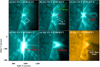 |
Fig. 8. Sequence of AIA 131 Å and 171 Å images showing the evolution of another X8.2 flare in AR 12673 on 2017 September 10. Multiple ejecta components and their counterparts before eruption are denoted by the pluses and arrows with different colors. The red arrows in panels d and e mark the current sheet and candle-flame-shaped structure in the decay phase of the flare. The AIA 171 Å image in panel f displays three groups of post-flare loops with different orientations. An animation (5.mpg) of the 171 Å and the 131 Å images is available online. |
The positive patch of “Dipole 3” moved southeastward while the negative one of “Dipole 4” moved toward the northwest, which then collided with each other eventually (panel d). Meanwhile, a new bipolar region “Dipole 5” emerged to the west of the positive patch of “Dipole 3” around September 5. We suggest that part of the loops connecting the opposite patches of “Dipole 5” would eventually evolve to LB1 due to the rotation of their footpoints. On September 6, the negative patch of “Dipole 4” quickly intruded into the northwest positive region (see the green solid arrow in panel e), which contributed to enhancement of Tw of FR1 and FR2 and led to the onset of the X9.3 flare as mentioned in Fig. 4. The velocity field in panel f derived from the DAVE method shows that the velocity of the patch’s motion reached up to ∼0.35 km s−1 at 10:59:04 UT, before the X9.3 flare’s onset.
3.4. The X8.2 flare on September 10
On September 10, an X8.2 flare took place in AR 12673, which was near the west solar limb. In this event, we also detect multiple ejecta components erupting consecutively and their counterparts (twisted structures) before the flare peaked at 16:06 UT (see Fig. 8 and the corresponding animation). These ejected structures were observed clearly in the 131 Å channel and separately denoted by the white, green, and red arrows in panels a–b). At about 15:35 UT, the emission at the north end of the twisted structure denoted by white arrows was enhanced. The brightening propagated southwards and traced out the whole structure, which kept rising slowly during the following ten minutes. Around 15:46 UT, another twisted structure marked by green arrows was illuminated. Then the two structures erupted outward with projected velocities of ∼250 km s−1 and ∼340 km s−1, respectively (see panel b). Meanwhile, one tear-drop-shaped structure appeared and rapidly moved outward with a velocity of ∼440 km s−1 (see panel c). After the eruption of the tear-drop-shaped structure, an evident current sheet was formed in the core region and lasted for several hours (panel d). Moreover, the post-flare candle-flame-shaped structure (Guidoni et al. 2015; Gou et al. 2015, 2016) was detected clearly in the 131 Å channel (see panel e). In the 171 Å channel, one can see three groups of post-flare loops with different orientations in the flaring region (see the arrows with different colors in panel f). These post-flare loops probably resulted from the eruptions of the multiple twisted structures mentioned above.
4. Conclusions and discussion
Employing the SDO observations, we investigate the two largest flares of Solar Cycle 24 occurring in AR 12673 and the evolution of the AR magnetic fields. On 2017 September 6, the largest flare of Solar Cycle 24 took place with its peak intensity reaching X9.3. Aided by NLFFF modeling, we identify a double-decker flux rope configuration above the PIL in the AR core region. The north ends of these two flux ropes were rooted at a negative magnetic patch, which began to move along the PIL and kept shearing with adjacent positive fields before the X9.3 flare on September 6. The strong shearing motion as well as a continuous rotation contributed together to the destabilization of the two magnetic flux ropes. Then the upper flux rope erupted upward due to the kink-instability and led to the successive eruptions of another two sets of twisted loop bundles beside the flux ropes within five minutes like a chain reaction. Similarly, during another X8.2 flare occurring on September 10, we also detected the successive eruptions of multiple ejecta components. The evolution of the AR magnetic fields shows that five dipoles emerged successively at the east of the main sunspot. The interactions between these dipoles took place continuously, accompanied by magnetic flux cancellations and strong shearing motions.
Flux ropes have been thought to be closely connected with CMEs and solar flares (Lin & Forbes 2000; Fan 2005; Liu 2013). Amari et al. (2000) proposed a model to approach the theory of CMEs and two-ribbon flares, in which twisted flux ropes play a crucial role. It was shown that the modeled magnetic configuration could not stay in equilibrium, and a considerable amount of magnetic energy was released during the eruption of the flux rope. Employing high-resolution observations from space platforms, Zhang et al. (2015) detected 1354 flux rope proxies over the solar disk from 2013 January to 2013 December. Hou et al. (2016) further implied the existence of multiple flux ropes during the evolution of AR 11897. The classical scenario assumes a single flux rope for each eruption, but it is easy to imagine multiple flux ropes if the AR is complex and has extended curved PIL (Liu et al. 2009, 2012; Shen et al. 2013; Awasthi et al. 2018). Török et al. (2011) presented a 3D MHD simulation to investigate three consecutive filament eruptions. They considered a configuration that contains two coronal flux ropes located within a pseudo-streamer and one rope located next to it. It is found that a sequence of eruptions was initiated by the eruption of the flux rope next to the streamer. The expansion of this rope resulted in two successive reconnection events, each of which triggered the eruption of a flux rope by reducing the overlying stabilizing flux. In the observational domain, Shen et al. (2012) reported the simultaneous occurrence of a partial and a full filament eruption in two neighboring source regions. Cheng et al. (2013) investigated successive eruptions of two flux ropes with an interval of several hours. In the present work, we identify a double-decker flux rope configuration above the PIL in the AR core region. The two flux ropes (FR1 and FR2) erupted at the onset of the X9.3 flare due to the shearing motion and rotation of the negative magnetic patch where the ropes were rooted. Then another two sets of twisted loop bundles (LB1 and LB2) beside these ropes were disturbed and successively erupted within five minutes like a chain reaction. The results from NLFFF modeling show that the ∣Tw∣ of FR1 and FR2 are beyond 1.0 and the ∣Ti∣ of LB1 is beyond 0.5. If we take a lower standard for defining a magnetic flux rope (e.g., Chintzoglou et al. 2015, who consider a half turn to be sufficient), then LB1 could be regarded as the third flux rope in this event. Therefore, we propose that the eruptions of a multi-flux-rope system rapidly released enormous magnetic energy and led to the X9.3 flare on September 6, the largest flare in Solar Cycle 24. Similar phenomenon was also observed during another X8.2 flare occurring in the same AR several days later.
In recent years, the concept of double-decker filament (flux rope) was proposed by Liu et al. (2012) to explain two vertically separated filaments (flux ropes) over the same PIL. The complex configuration of double-decker flux rope was observed and modeled to exist prior to solar eruptive events (Cheng et al. 2014; Kliem et al. 2014). Extrapolated NLFFF structures in this work reveal that before the onset of the X9.3 flare, two magnetic flux ropes were located separated vertically above the PIL in the AR core region, forming a typical double-decker flux rope configuration. At the onset of the X9.3 flare, the strong shearing motion and rotation of the north ends of the two magnetic flux ropes contributed to their destabilization (Kliem et al. 2004; Srivastava et al. 2010; Török et al. 2013; Yan et al. 2018b). The brightening at the cross sites of these two ropes observed in EUV wavelength indicated the interaction (magnetic reconnection) occurring between the two flux ropes during their slow-rise phase. The subsequent AIA observations revealed that the lower rope lost its stability first and erupted outwards while the upper flux rope kept rising upward. Then the upper magnetic flux rope writhed into a sigmoid shape. The calculation of twist number based on the NLFFF results shows that the maximum ∣Tw∣ of the two flux ropes were all beyond 1.75 half an hour before the onset of the flare. It is worth noting that the exact value of twist required of the kink instability depends on various factors such as the flux rope geometry and the surrounding magnetic fields. Török et al. (2004) proposed that the threshold of instability increases with rising aspect ratio and the number is 1.75 (3.5π) at a loop aspect ratio R/a ≈ 5, which corresponds to a rather fat flux rope. Although the double-decker flux ropes in the present work may have a different aspect ratio, we approximate the threshold value of kink instability to 1.75 here. The facts that the twist of the flux rope is beyond the threshold value of kink instability and its conversion into the writhe support the occurrence of the kink instability during the eruption of the upper flux rope. The eruption of a kink-unstable flux rope during this event has also been investigated by Yang et al. (2017).
The existence of multiple flux ropes and twisted loop bundles during the two X-class flares reported in the present paper implies a complicated magnetic system in AR 12673. Examining the evolution of the magnetic fields in the AR core region, we notice that significant flux emergence occurred in this region (Sun & Norton 2017). Five dipoles emerged successively at the east of the main sunspot. The negative and positive patches of the first two dipoles separated along the east-west direction. However, the patches of the latter two dipoles separated along the north-south direction, perpendicular to the former one. The cross separation of these dipole patches with opposite polarities led to the continuous interactions between different dipolar fields, accompanied by magnetic flux cancellations at some places (Toriumi et al. 2013; Louis et al. 2015; Yang et al. 2017). Strong shearing motions between the patches with opposite polarities accumulated dramatic free energy (Shimizu et al. 2014; Toriumi & Takasao 2017) and could result in magnetic reconnection (Moore et al. 2001), which would lead to the formation of flux ropes (Xue et al. 2017). The rotation of the associated magnetic patch also contributes to the magnetic flux rope buildup. In Sect. 3.3, we speculated on the detailed process concerning the formations of these flux ropes and twisted loop bundles. It is worth mentioning that during the impulsive phase of the X9.3 flare, a white-light signal was detected as well as anomalous magnetic transient near the PIL (see the animation corresponding to Fig. 4), indicating a violent release of energy (Hudson et al. 1992; Song et al. 2018). We propose that in AR 12673 significant flux emergence and successive cross-separations between the patches of different newly emerging dipoles resulted in the formation of multiple flux ropes and twisted loop bundles in the same AR and the storage of dramatic magnetic energy.
Movies
Movie of Fig. 3 Access Supplementary Material
Movie of Fig. 4 Access Supplementary Material
Movie of Fig. 5 Access Supplementary Material
Movie of Fig. 7 Access Supplementary Material
Movie of Fig. 8 Access Supplementary Material
Acknowledgments
The authors are grateful to the anonymous referee for valuable suggestions. The data are used courtesy of the SDO and GOES science teams. SDO is a mission of NASA’s Living With a Star Program. This work is supported by the National Natural Science Foundations of China (11533008, 11790304, 11773039, 11673035, 11673034, 11873059, and 11790300), the Youth Innovation Promotion Association of CAS (2017078 and 2014043), and Key Programs of the Chinese Academy of Sciences (QYZDJ-SSW-SLH050).
References
- Alexander, D., Liu, R., & Gilbert, H. R. 2006, ApJ, 653, 719 [NASA ADS] [CrossRef] [Google Scholar]
- Amari, T., Luciani, J. F., Mikic, Z., & Linker, J. 2000, ApJ, 529, L49 [NASA ADS] [CrossRef] [PubMed] [Google Scholar]
- Amari, T., Luciani, J. F., Aly, J. J., Mikic, Z., & Linker, J. 2003, ApJ, 585, 1073 [NASA ADS] [CrossRef] [Google Scholar]
- Aulanier, G., Török, T., Démoulin, P., & DeLuca, E. E. 2010, ApJ, 708, 314 [Google Scholar]
- Awasthi, A. K., Liu, R., Wang, H., Wang, Y., & Shen, C. 2018, ApJ, 857, 124 [NASA ADS] [CrossRef] [Google Scholar]
- Baty, H. 2001, A&A, 367, 321 [NASA ADS] [CrossRef] [EDP Sciences] [Google Scholar]
- Berger, M. A., & Prior, C. 2006, J. Phys. A, 39, 8321 [Google Scholar]
- Bobra, M. G., Sun, X., Hoeksema, J. T., et al. 2014, Sol. Phys., 289, 3549 [NASA ADS] [CrossRef] [Google Scholar]
- Brown, D. S., Nightingale, R. W., Alexander, D., et al. 2003, Sol. Phys., 216, 79 [NASA ADS] [CrossRef] [Google Scholar]
- Chen, P. F., & Shibata, K. 2000, ApJ, 545, 524 [Google Scholar]
- Cheng, X., Zhang, J., Liu, Y., & Ding, M. D. 2011, ApJ, 732, L25 [NASA ADS] [CrossRef] [Google Scholar]
- Cheng, X., Zhang, J., Ding, M. D., et al. 2013, ApJ, 769, L25 [NASA ADS] [CrossRef] [Google Scholar]
- Cheng, X., Ding, M. D., Zhang, J., et al. 2014, ApJ, 789, 93 [NASA ADS] [CrossRef] [Google Scholar]
- Chintzoglou, G., Patsourakos, S., & Vourlidas, A. 2015, ApJ, 809, 34 [NASA ADS] [CrossRef] [Google Scholar]
- Fan, Y. 2005, ApJ, 630, 543 [NASA ADS] [CrossRef] [Google Scholar]
- Fan, Y., & Gibson, S. E. 2004, ApJ, 609, 1123 [NASA ADS] [CrossRef] [Google Scholar]
- Forbes, T. G., & Priest, E. R. 1995, ApJ, 446, 377 [NASA ADS] [CrossRef] [Google Scholar]
- Gou, T., Liu, R., & Wang, Y. 2015, Sol. Phys., 290, 2211 [NASA ADS] [CrossRef] [Google Scholar]
- Gou, T., Liu, R., Wang, Y., et al. 2016, ApJ, 821, L28 [NASA ADS] [CrossRef] [Google Scholar]
- Green, L. M., Kliem, B., & Wallace, A. J. 2011, A&A, 526, A2 [NASA ADS] [CrossRef] [EDP Sciences] [Google Scholar]
- Guglielmino, S. L., Romano, P., & Zuccarello, F. 2017, ApJ, 846, L16 [NASA ADS] [CrossRef] [Google Scholar]
- Guidoni, S. E., McKenzie, D. E., Longcope, D. W., Plowman, J. E., & Yoshimura, K. 2015, ApJ, 800, 54 [NASA ADS] [CrossRef] [Google Scholar]
- Guo, Y., Schmieder, B., Démoulin, P., et al. 2010, ApJ, 714, 343 [NASA ADS] [CrossRef] [Google Scholar]
- Guo, Y., Ding, M. D., Cheng, X., Zhao, J., & Pariat, E. 2013, ApJ, 779, 157 [NASA ADS] [CrossRef] [Google Scholar]
- Hoeksema, J. T., Liu, Y., Hayashi, K., et al. 2014, Sol. Phys., 289, 3483 [Google Scholar]
- Hood, A. W., & Priest, E. R. 1979, Sol. Phys., 64, 303 [NASA ADS] [CrossRef] [Google Scholar]
- Hou, Y. J., Li, T., & Zhang, J. 2016, A&A, 592, A138 [Google Scholar]
- Hudson, H. S., Acton, L. W., Hirayama, T., & Uchida, Y. 1992, PASJ, 44, L77 [NASA ADS] [Google Scholar]
- Jiang, C., Zou, P., & Feng, X. 2018, ApJ, submitted [Google Scholar]
- Kliem, B., Titov, V. S., & Török, T. 2004, A&A, 413, L23 [NASA ADS] [CrossRef] [EDP Sciences] [Google Scholar]
- Kliem, B., Linton, M. G., Török, T., & Karlický, M. 2010, Sol. Phys., 266, 91 [NASA ADS] [CrossRef] [Google Scholar]
- Kliem, B., Török, T., Titov, V. S., et al. 2014, ApJ, 792, 107 [NASA ADS] [CrossRef] [Google Scholar]
- Kumar, P., & Cho, K.-S. 2014, A&A, 572, A83 [NASA ADS] [CrossRef] [EDP Sciences] [Google Scholar]
- Kumar, P., Yurchyshyn, V., Cho, K.-S., & Wang, H. 2017, A&A, 603, A36 [NASA ADS] [CrossRef] [EDP Sciences] [Google Scholar]
- Leka, K. D., Fan, Y., & Barnes, G. 2005, ApJ, 626, 1091 [NASA ADS] [CrossRef] [Google Scholar]
- Lemen, J. R., Title, A. M., Akin, D. J., et al. 2012, Sol. Phys., 275, 17 [NASA ADS] [CrossRef] [Google Scholar]
- Li, L. P., & Zhang, J. 2013a, A&A, 552, L11 [NASA ADS] [CrossRef] [EDP Sciences] [Google Scholar]
- Li, T., & Zhang, J. 2013b, ApJ, 778, L29 [NASA ADS] [CrossRef] [Google Scholar]
- Li, T., Yang, K., Hou, Y., & Zhang, J. 2016, ApJ, 830, 152 [NASA ADS] [CrossRef] [Google Scholar]
- Lin, J., & Forbes, T. G. 2000, Geophys. Res., 105, 2375 [NASA ADS] [CrossRef] [Google Scholar]
- Liu, R. 2013, MNRAS, 434, 1309 [NASA ADS] [CrossRef] [Google Scholar]
- Liu, R., Alexander, D., & Gilbert, H. R. 2007, ApJ, 661, 1260 [NASA ADS] [CrossRef] [Google Scholar]
- Liu, C., Lee, J., Karlický, M., et al. 2009, ApJ, 703, 757 [NASA ADS] [CrossRef] [Google Scholar]
- Liu, R., Liu, C., Wang, S., Deng, N., & Wang, H. 2010, ApJ, 725, L84 [NASA ADS] [CrossRef] [Google Scholar]
- Liu, R., Kliem, B., Török, T., et al. 2012, ApJ, 756, 59 [NASA ADS] [CrossRef] [Google Scholar]
- Liu, Y., Zhao, J., & Schuck, P. W. 2013, Sol. Phys., 287, 279 [NASA ADS] [CrossRef] [Google Scholar]
- Liu, R., Kliem, B., Titov, V. S., et al. 2016, ApJ, 818, 148 [NASA ADS] [CrossRef] [Google Scholar]
- Louis, R. E., Kliem, B., Ravindra, B., & Chintzoglou, G. 2015, Sol. Phys., 290, 3641 [Google Scholar]
- Meunier, N., & Kosovichev, A. 2003, A&A, 412, 541 [NASA ADS] [CrossRef] [EDP Sciences] [Google Scholar]
- Moore, R. L., Sterling, A. C., Hudson, H. S., & Lemen, J. R. 2001, ApJ, 552, 833 [NASA ADS] [CrossRef] [Google Scholar]
- Pesnell, W. D., Thompson, B. J., & Chamberlin, P. C. 2012, Sol. Phys., 275, 3 [NASA ADS] [CrossRef] [Google Scholar]
- Priest, E. R., & Forbes, T. G. 2002, A&ARv, 10, 313 [NASA ADS] [CrossRef] [Google Scholar]
- Schmieder, B., Aulanier, G., & Vršnak, B. 2015, Sol. Phys., 290, 3457 [Google Scholar]
- Schou, J., Scherrer, P. H., Bush, R. I., et al. 2012, Sol. Phys., 275, 229 [Google Scholar]
- Schuck, P. W. 2006, ApJ, 646, 1358 [NASA ADS] [CrossRef] [Google Scholar]
- Shen, Y., Liu, Y., & Su, J. 2012, ApJ, 750, 12 [NASA ADS] [CrossRef] [Google Scholar]
- Shen, C., Li, G., Kong, X., et al. 2013, ApJ, 763, 114 [NASA ADS] [CrossRef] [Google Scholar]
- Shen, Y., Liu, Y., Song, T., & Tian, Z. 2018a, ApJ, 853, 1 [NASA ADS] [CrossRef] [Google Scholar]
- Shen, C., Xu, M., Wang, Y., Chi, Y., & Luo, B. 2018b, ApJ, 861, 28 [NASA ADS] [CrossRef] [Google Scholar]
- Shimizu, T., Lites, B. W., & Bamba, Y. 2014, PASJ, 66, S14 [NASA ADS] [CrossRef] [Google Scholar]
- Song, Y. L., Guo, Y., Tian, H., et al. 2018, ApJ, 854, 64 [NASA ADS] [CrossRef] [Google Scholar]
- Srivastava, A. K., Zaqarashvili, T. V., Kumar, P., & Khodachenko, M. L. 2010, ApJ, 715, 292 [NASA ADS] [CrossRef] [Google Scholar]
- Sterling, A. C., Chifor, C., Mason, H. E., Moore, R. L., & Young, P. R. 2010, A&A, 521, A49 [NASA ADS] [CrossRef] [EDP Sciences] [Google Scholar]
- Sun, X., & Norton, A. A. 2017, Res. Notes Am. Astron. Soc., 1, 24 [NASA ADS] [CrossRef] [Google Scholar]
- Sun, X., Hoeksema, J. T., Liu, Y., et al. 2012, ApJ, 748, 77 [NASA ADS] [CrossRef] [Google Scholar]
- Toriumi, S., & Takasao, S. 2017, ApJ, 850, 39 [NASA ADS] [CrossRef] [Google Scholar]
- Toriumi, S., Iida, Y., Bamba, Y., et al. 2013, ApJ, 773, 128 [NASA ADS] [CrossRef] [Google Scholar]
- Török, T., Kliem, B., & Titov, V. S. 2004, A&A, 413, L27 [NASA ADS] [CrossRef] [EDP Sciences] [Google Scholar]
- Török, T., Panasenco, O., Titov, V. S., et al. 2011, ApJ, 739, L63 [NASA ADS] [CrossRef] [Google Scholar]
- Török, T., Temmer, M., Valori, G., et al. 2013, Sol. Phys., 286, 453 [NASA ADS] [CrossRef] [Google Scholar]
- Verma, M. 2018, A&A, 612, A101 [NASA ADS] [CrossRef] [EDP Sciences] [Google Scholar]
- Wang, J., & Shi, Z. 1993, Sol. Phys., 143, 119 [NASA ADS] [CrossRef] [Google Scholar]
- Wang, H., Ewell, M. W. Jr, Zirin, H., & Ai, G. 1994, ApJ, 424, 436 [NASA ADS] [CrossRef] [Google Scholar]
- Wang, W., Liu, R., Wang, Y., et al. 2017a, Nat. Comms., 8, 1330 [Google Scholar]
- Wang, W., Liu, R., & Wang, Y. 2017b, ApJ, 834, 38 [NASA ADS] [CrossRef] [Google Scholar]
- Wang, H., Yurchyshyn, V., Liu, C., et al. 2018, Res. Notes Am. Astron. Soc., 2, 8 [CrossRef] [Google Scholar]
- Wiegelmann, T. 2004, Sol. Phys., 219, 87 [NASA ADS] [CrossRef] [Google Scholar]
- Wiegelmann, T., Inhester, B., & Sakurai, T. 2006, Sol. Phys., 233, 215 [NASA ADS] [CrossRef] [Google Scholar]
- Wiegelmann, T., Thalmann, J. K., Inhester, B., et al. 2012, Sol. Phys., 281, 37 [NASA ADS] [Google Scholar]
- Xue, Z., Yan, X., Yang, L., Wang, J., & Zhao, L. 2017, ApJ, 840, L23 [NASA ADS] [CrossRef] [Google Scholar]
- Yan, X. L., Jiang, C. W., Xue, Z. K., et al. 2017, ApJ, 845, 18 [NASA ADS] [CrossRef] [Google Scholar]
- Yan, X. L., Yang, L. H., Xue, Z. K., et al. 2018a, ApJ, 853, L18 [NASA ADS] [CrossRef] [Google Scholar]
- Yan, X. L., Wang, J. C., Pan, G. M., et al. 2018b, ApJ, 856, 79 [NASA ADS] [CrossRef] [Google Scholar]
- Yang, S., Zhang, J., Liu, Z., & Xiang, Y. 2014, ApJ, 784, L36 [NASA ADS] [CrossRef] [Google Scholar]
- Yang, S., Zhang, J., Zhu, X., & Song, Q. 2017, ApJ, 849, L21 [NASA ADS] [CrossRef] [Google Scholar]
- Zhang, J., Wang, J., Deng, Y., & Wu, D. 2001, ApJ, 548, L99 [NASA ADS] [CrossRef] [Google Scholar]
- Zhang, J., Li, L., & Song, Q. 2007, ApJ, 662, L35 [NASA ADS] [CrossRef] [Google Scholar]
- Zhang, J., Cheng, X., & Ding, M.-D. 2012, Nat. Comm., 3, 747 [Google Scholar]
- Zhang, J., Yang, S. H., & Li, T. 2015, A&A, 580, A2 [NASA ADS] [CrossRef] [EDP Sciences] [Google Scholar]
All Figures
|
Fig. 1. Flares produced by AR 12673. Panel a: GOES SXR 1–8 Å flux variation from 2017 September 3 to September 11. Four X-class flares took place during this period, of which the two largest ones reached up to X9.3 (orange region) and X8.2 (green region), respectively. The blue horizontal dotted lines mark the threshold levels of M1.0 and X1.0 flares. Panels b–d: overview of the X9.3 flare in AR 12673 on September 6. The AIA 94 Å image in panel b shows this AR at the onset of the flare. HMI continuum intensitygram and LOS magnetogram in panels c and d display the sunspots and underlying magnetic fields in the AR core region, whose field of view (FOV) is outlined by the green square in panel b. |
| In the text | |
|
Fig. 2. Double-decker flux rope configuration above the PIL in the AR core region revealed by NLFFF modeling at 11:24 UT on 2017 September 6. Panels a–b: top view and side view of two flux ropes (FR1 and FR2) composing the double-decker configuration. The FOV of these panels is approximated by the white square in Fig. 1d. Panel c: isosurfaces of twist number Tw = –1 (white) and Tw = –1.75 (red) viewed from the same perspective as panel a. Panel d: twist number distribution in the vertical (x–z) plane along the green cut labeled in panel c. |
| In the text | |
|
Fig. 3. Eruption of the double-decker flux rope configuration. Panels a1 –a7: sequence of extended AIA 304 Å images showing the filament and eruption process of the double-decker flux rope configuration. The two filaments and associated brightening before their eruption are denoted by green arrows in panels a1 –a4. The green curves in panels a6 and a7 delineate the twisted threads and the writhed structure of the upper flux rope (FR2). Panel b: corresponding 94 Å image exhibiting the double-decker flux rope configuration in a higher temperature wavelength. The FOV is outlined by the white square in Fig. 1(d). An animation (1.mpg) of the 304 Å and the 94 Å images is available online. |
| In the text | |
|
Fig. 4. Magnetic evolution of the AR core region during the X9.3 flare. Panels a1 –a3: HMI LOS magnetograms with contours of ± 400 G displaying the magnetic fields of the core region before and after the flare peak at 12:02 UT. The green solid arrows in panels a1 and a3 denote the direction of rapid displacement of the negative patch where the north ends of the double-decker flux rope configuration are rooted. The green arrows in panel a2 mark the magnetic transients caused by the white-light flare. Panels b1–b2: corresponding HMI continuum intensitygrams. The green arrow in panel b1 labels the rotation of the negative patch. The red arrows in panel b2 mark the signals of the white-light flare. Panel c: the horizontal photospheric velocity field (colored arrows) derived from the HMI continuum intensitygrams computed by the DAVE method. In the lower-left corner, the radius of the circle corresponds to a speed of 0.3 km s−1, and the color of an arrow corresponds to its direction. The FOV is the same as Fig. 3. An animation (2.mpg) of the HMI continuum intensitygrams and LOS magnetograms is available online. |
| In the text | |
|
Fig. 5. Dynamic evolutions of the complex system consisting of multiple flux ropes and twisted loop bundles during the X9.3 flare. Panels a1 –a3: sequence of AIA 94 Å images showing the interaction between FR2 and the first twisted loop bundles (LB1). The red curves delineate their main axes. The white solid arrows in panel a1 mark the rising directions of FR2. The white arrows in panels a2–a3 denote the moving direction of LB1 after the interaction with FR2. Panels b1–b3: 94 Å images with a larger FOV exhibiting LB1 and the second twisted loop bundles (LB2). The green square in panel b2 outlines the FOV of panels a1– a3. Panels d1–d2: time-space plots along arc-sector domains “A–B” of panel b1 and “C–D” of panel b3 in 94 Å channel. The red lines approximate trajectories of FR2, LB1, and LB2. The full temporal evolution of the 94 Å images is available as an online movie (3.mpg). |
| In the text | |
|
Fig. 6. Extrapolated 3D NLFFF structures corresponding to FR1, FR2, LB1, and LB2 at 11:24 UT on 2017 September 6. Panel a: shows these structures from a top view, and panel b shows them from a side view. The FOV of this figure is similar to that of Figs. 1c–d. |
| In the text | |
|
Fig. 7. Sequence of HMI LOS magnetograms displaying the evolution of magnetic fields in AR 12673 from September 3 to September 6. The red and blue curves are contours of the LOS magnetograms at +500 and −500 G, respectively. Five newly emerging dipoles are marked by green arrows. The green solid arrow in panel e denotes the moving direction of the negative patch of “Dipole 4”. Panel f: shows the horizontal photospheric velocity field (colored arrows) derived from the HMI LOS magnetograms computed by the DAVE method. Arrows are only superimposed at locations where the absolute value of magnetic field is greater than 1000 G and illustrate the horizontal flows around 10:59:04 UT on September 6. The FOV of these panels is the same as that of Figs. 1c–d. The temporal evolution of the HMI intensitygrams and HMI LOS magnetograms is available as an online movie (4.mpg). |
| In the text | |
|
Fig. 8. Sequence of AIA 131 Å and 171 Å images showing the evolution of another X8.2 flare in AR 12673 on 2017 September 10. Multiple ejecta components and their counterparts before eruption are denoted by the pluses and arrows with different colors. The red arrows in panels d and e mark the current sheet and candle-flame-shaped structure in the decay phase of the flare. The AIA 171 Å image in panel f displays three groups of post-flare loops with different orientations. An animation (5.mpg) of the 171 Å and the 131 Å images is available online. |
| In the text | |
Current usage metrics show cumulative count of Article Views (full-text article views including HTML views, PDF and ePub downloads, according to the available data) and Abstracts Views on Vision4Press platform.
Data correspond to usage on the plateform after 2015. The current usage metrics is available 48-96 hours after online publication and is updated daily on week days.
Initial download of the metrics may take a while.