| Issue |
A&A
Volume 618, October 2018
|
|
|---|---|---|
| Article Number | A157 | |
| Number of page(s) | 15 | |
| Section | Extragalactic astronomy | |
| DOI | https://doi.org/10.1051/0004-6361/201833329 | |
| Published online | 25 October 2018 | |
Improving Hickson-like compact group finders in redshift surveys: an implementation in the SDSS⋆
1
Instituto de Astronomía Teórica y Experimental (IATE), CONICET-UNC, Argentina
e-mail: eugeniadiazz@gmail.com
2
Observatorio Astronómico de Córdoba (OAC), Universidad Nacional de Córdoba (UNC), Córdoba, Argentina
3
Facultad de Matemática, Astronomía, Física y Computación (FaMAF), Universidad Nacional de Córdoba (UNC), Córdoba, Córdoba
Received:
30
April
2018
Accepted:
16
August
2018
Aims. In this work we present an algorithm to identify compact groups (CGs) that closely follows Hickson’s original aim and that improves the completeness of the samples of compact groups obtained from redshift surveys.
Methods. Instead of identifying CGs in projection first and then checking a velocity concordance criterion, we identify them directly in redshift space using Hickson-like criteria. The methodology was tested on a mock lightcone of galaxies built from the outputs of a recent semi-analytic model of galaxy formation run on top of the Millennium Simulation I after scaling to represent the first-year Planck cosmology.
Results. The new algorithm identifies nearly twice as many CGs, no longer missing CGs that failed the isolation criterion because of velocity outliers lying in the isolation annulus. The new CG sample picks up lower surface brightness groups, which are both looser and with fainter brightest galaxies, missed by the classic method. A new catalogue of compact groups from the Sloan Digital Sky Survey is the natural corollary of this study. The publicly available sample comprises 462 observational groups with four or more galaxy members, of which 406 clearly fulfil all the compact group requirements: compactness, isolation, and velocity concordance of all of their members. The remaining 56 groups need further redshift information of potentially contaminating sources. This constitutes the largest sample of groups that strictly satisfy all the Hickson’s criteria in a survey with available spectroscopic information.
Key words: galaxies: groups: general / catalogs / methods: statistical / methods: data analysis
Full Tables D.1 and D.2 are only available at the CDS via anonymous ftp to cdsarc.u-strasbg.fr (130.79.128.5) or via http://cdsarc.u-strasbg.fr/viz-bin/qcat?J/A+A/618/A157
© ESO 2018
1. Introduction
Over the past 40 years, the astronomical community has devoted much time to the systematic search for compact groups (CGs). These peculiar small galaxy systems have proven to be a very powerful tool to understand galaxy interactions in dense environments, shaping our knowledge of galaxy evolution.
The most popular sample of CGs was identified by Hickson (1982). This sample was a systematic search of CGs on plates of the Palomar Observatory Sky Survey that relied on a visual inspection. Hickson established a set of rules that should be fulfilled for a galaxy system to be considered a compact group: compactness, isolation (with a relatively empty annulus surrounding the group), and population. These rules were defined to obtain small, isolated, and compact galaxy systems. In this way, Hickson created the well-known Hickson Compact Group (HCG) sample that comprises 100 galaxy groups identified in projection on the sky. However, since only angular positions were used to identify the sample, their truly compact nature was questioned (e.g. Mamon 1986, 1990). A few years later, the red-shifts of their galaxy members were measured and a velocity filter was added to the criteria, resulting in a sample of 68 CGs with at least four concordant velocities (Hickson et al. 1992).
Since then, several works have identified CGs in observational or simulated galaxy catalogues based on Hickson’s recipes with or without including the velocity filtering depending on the available information (e.g. Prandoni et al. 1994; Iovino 2002; Lee et al. 2004; McConnachie et al. 2008, 2009; DíazGiménez & Mamon 2010; Díaz-Giménez et al. 2012; Sohn et al. 2015). Most of these works share the same philosophy for the algorithm construction, i.e. finding CGs that meet Hickson’s criteria through an automatic procedure that resembles the original Hickson’s visual inspection by first detecting candidate CGs on the sky, and then discarding obvious foreground/background galaxies along the line of sight from their discordant redshifts. However, for quasi-complete spectroscopic galaxy catalogues this procedure is not optimal because it may discard groups that appear not isolated on the sky, although the galaxies populating the isolation annulus turn out to all have discordant redshifts. Having chance projected galaxies in the cone is not a problem if subsequent velocity filtering is performed. The big problem is that if such galaxies lie outside the CG, they will lead the algorithm to discard the group as non-isolated, whereas they are clear chance projections along the line of sight. The type of restrictions that arises from the procedure itself could easily bias subsequent studies related to CGs environment.
In the past, some authors already noticed this problem and suggested new ways to identify CGs in redshift surveys by changing the searching procedure and using percolation algorithms similar to the friends-of-friends (FoF) algorithm (e.g. Barton et al. 1996; Focardi & Kelm 2002; Zandivarez et al. 2003; Sohn et al. 2016). However, most of these attempts disregarded most or all of Hickson’s definitions, and only kept a compactness criterion based on the physical size of the galaxy systems or the intergalactic separations.
The purpose of the present work is to present a modified algorithm that applies the Hickson’s criteria directly in redshift space. As a result, we present a new catalogue of CGs extracted from the Sloan Digital Sky Survey (SDSS) that satisfies Hickson’s criteria.
The layout of this work is as follows. In Sect. 2 we describe the construction of the mock galaxy lightcone used in this work for the testing process. This catalogue was constructed using synthetic galaxies obtained from a semi-analytical model (SAM) of galaxy formation (Henriques et al. 2015). In Sect. 3 we describe the well-known Hickson’s recipe for identifying CGs (Hickson 1982; Hickson et al. 1992) and the previous and new algorithms for identifying CGs that fulfil these conditions. We apply these algorithms to the mock catalogue and perform the corresponding comparisons between the resulting CG catalogues. In Sect. 4 we apply both algorithms to an observational galaxy sample compiled from the SDSS by Tempel et al. (2017) and compare the resulting new CG sample with previous observational identifications. Finally, in Sect. 5 we summarise our results and present our conclusions.
2. Mock galaxy catalogue
Using the publicly available outputs of the SAM of Henriques et al. (2015) run on the N-body Millennium simulation (Springel et al. 2005) re-scaled to the Planck cosmology1, we construct a mock lightcone galaxy catalogue following a procedure similar to that described in Zandivarez et al. (2014a); see subsection 2.3 for details). The lightcone was built using galaxies extracted from different redshift outputs of the simulation to include the evolution of structures and galaxy properties with time.
The lightcone is limited to an SDSS r-band observer-frame AB apparent magnitude of r < 17.77. To compute the observer-frame magnitudes in the lightcones, it is necessary to k-decorrect the rest-frame magnitudes provided by the SAM. An iterative process is used to compute the k-corrections, and therefore the observer-frame magnitudes. A detailed description of this procedure is included in Appendix A.
The final sample comprises 3 139 409 galaxies within a solid angle of 4π sr.
3. Compact group finder algorithms
Hickson-like CGs are expected to meet the following criteria:
Population: 4 ≤ N ≤ 10;
Compactness: μr ≤ μlim;
Isolation: Θn > 3 ΘG;
Flux limit: rb ≤ rlim − 3;
Velocity filtering:  .
.
Here, N is the number of galaxies whose r-band magnitudes are within a three-magnitude range from the brightest galaxy; μr is the mean r-band surface brightness averaged over the smallest circle that circumscribes the galaxy centres; ΘG is the angular diameter of the smallest circumscribed circle; Θn is the angular diameter of the largest concentric circle that contains no other galaxies within the considered magnitude range or brighter; rb is the apparent magnitude of the brightest galaxy of the group; rlim is the apparent magnitude limit of the parent catalogue, in our case rlim = 17.77; zi is the spectroscopic redshift of each galaxy member; and 〈zcm〉 is the median of the redshifts of the galaxy members. The flux limit criterion has to be included to ensure the membership and isolation of the groups since the population and isolation criteria are checked against galaxies within a three-magnitude range from the brightest (DíazGiménez & Mamon 2010). The value of μlim (surface brightness limit) depends on the photometric band in which the selection is made. In our case, we work on the r band; therefore, the adopted limit is μlim = 26.33 [mag arcsec−2] (Taverna et al. 2016).
Different algorithms can be applied in order to produce a sample of CGs that meets all the criteria described above. As we will show later, the order in which the criteria are applied affects the completeness of the resulting sample.
3.1. Classic algorithm
In several previous works (DíazGiménez & Mamon 2010; Díaz-Giménez et al. 2012; Zandivarez et al. 2014b; DíazGiménez & Zandivarez 2015; Taverna et al. 2016), we applied an algorithm to produce samples of Hickson-like compact groups. Following the original procedure, we identified CGs in projection on the plane of sky that met the first four criteria mentioned above, and we applied the velocity filtering only in a second stage.
The description of our algorithm can be found in DíazGiménez & Mamon (2010). Hereafter, we refer to this method as Hickson Classic (HC). Its full implementation is shown in the flow chart in Fig. 1 (left). The algorithm starts looking for the smallest CGs; it starts with only four galaxies and it checks all the CG criteria. If the isolation is not fulfilled, it might eventually include new galaxy members or discard the CG. In a subsequent stage, it is checked for embedded compact groups: there could be CGs contained within a larger CG. We detected these cases, and adopted the largest ones. Finally, for these projected compact groups, a velocity filtering is applied through an iterative procedure that discards the farthest inter-loper and checks compactness, population, and velocity again.
When working with mock galaxy catalogues, it is also necessary to take into consideration that galaxies in the mock catalogue are just point-sized particles, while observed galaxies are extended objects. Following DíazGiménez & Mamon (2010) we therefore included the blending of galaxies in projection on the plane of the sky, which modifies the number of detectable galaxies and changes the population of CGs. To examine whether two galaxies are blended, we first computed the half-light radii in the r band as a function of the stellar mass of each mock galaxy following the prescriptions of Lange et al. (2015; see their Eqs. (20) and (3)), using the bulge-to-total stellar mass ratio as a proxy for morphological type (Bertone et al. 2007). Finally, we considered that two galaxies are blended if their angular separation is smaller than the sum of their angular half-light radii. The number of members is recomputed considering the galaxies that have been blended, and groups whose population is less than four galaxies are discarded. The blending is checked twice, once when the projected compact groups are identified, and again after applying the velocity filter.
The application of the classic algorithm leads to a final sample that comprises 680 mock Hickson classic compact groups (mHCCGs) in the lightcone described in Sect. 2 (see Table 1).
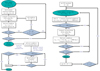 |
Fig. 1. Flow charts showing the automatic implementation of the Hickson’s criteria to identify CGs. On the left the flow chart shows the classic algorithm, while on the right the modified algorithm is shown. |
Number of CGs identified using the classic and modified algorithms.
3.2. Modified algorithm
Our implementation of the classic algorithm was inspired by the original path followed by Hickson at a time when red-shift surveys were not available. Different authors were able to create new samples following the same automatic methodology applied on different galaxy catalogues (McConnachie et al. 2009; Díaz-Giménez et al. 2012).
However, the availability of large redshift surveys allows the CG finder algorithm to be simplified and improved. Given that the CG criteria involve the counting of galaxies within a projected area on the sky, not taking into account the position of galaxies along the line of sight leads to losing groups by including interlopers, either as galaxy members or as breaches of the isolation.
In our modified algorithm (hereafter Hickson Modified (HM)), we therefore consider the redshifts of galaxies from the very beginning of the implementation. Galaxies considered to be neighbours (for membership and isolation) are taken from a cylinder in redshift space around the point where the criteria are being evaluated. Therefore, the velocity filtering is applied at the same time as the other constraints. In the implementation of the new algorithm we also introduce another change to automatically obtain the largest compact groups in one single run; in the classic implementation it was run a posteriori. Therefore, we start looking for the largest CGs, and then we select the smaller CG not contained in any previously found larger CG. This is achieved by identifying CGs with the largest numbers of members at first (N = 10), and then looking for groups with gradually fewer members. In Fig. 1, the flow chart that schematises the algorithm is shown on the right.
As we mentioned above, when the algorithm is applied to a mock lightcone, the blending of galaxies has to be introduced after identifying the CGs to discard those groups whose membership falls below the lower limit when galaxies are blended.
The sample identified in the mock lightcone using this modified algorithm comprises 1287 mHMCGs (Table 1).
3.3. Comparison of the classic and modified compact group samples
In this section we compare the two samples of CGs obtained using different algorithms. To start with, we note that the modified algorithm produces a sample that is 89% larger than the classic sample. We cross-correlated the two samples and considered that a group from one sample has been recovered in the other sample if the angular distance between their centres are less than the sum of the angular radii of the groups. By cross-correlating the samples, we found that 95% of the classic sample (647 mHCCGs) is included in the modified sample. This means that the new algorithm is able to recover most of the classic sample, but it also identifies almost twice the number of groups, improving the statistics significantly. We also analysed the reasons why the classic algorithm misses almost half of the mHMCGs. We found that 90% of the missing groups are discarded by the classic algorithm because there are discordant-velocity galaxies contaminating the isolation annulus in projection. In the remaining 10%, the membership was compromised: some of the true group galaxy members were identified in projection, but others were missing, and new discordant redshift galaxies were included as group galaxy members. These groups did not pass the posterior velocity filtering.
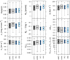 |
Fig. 2. Boxplot diagrams of CG properties for groups identified using the classic and the modified algorithm. The notches (waists) in the boxes indicate ∼95 % confidence intervals for the medians, while the widths are proportional to the square roots of the number of objects in each sample (R Core Team 2013). The boxplot diagrams on the left side in each panel are the samples obtained using the classic and the modified algorithms in the mock catalogue (mHC and mHM), while those at the right side show the results for the samples obtained applying both algorithms on the SDSS catalogue (HC and HM). |
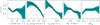 |
Fig. 3. Ratio of the classic to the modified distributions for a given property. Shaded areas correspond to the errors computed using the error propagation formula for the ratio (each number in the ratio has a Poisson error). |
As suggested by Mamon (1986) for the HCG sample, a non-negligible fraction of mock CGs are chance projections along the line of sight (McConnachie et al. 2008; DíazGiménez & Mamon 2010). It is interesting to examine whether the different algorithms might lead to different percentages of contamination. Following the classification in 3D real space in the simulations performed by DíazGiménez & Mamon (2010), we split the sample into real CGs2 and chance alignments. We found that (38 ± 3)% of the mHCCGs (256) are real, while (35 ± 2)% of the mHMCGs (452) can be classified as real (Table 1)3. Therefore, the percentage of physically dense groups is unaffected by the algorithm.
In Fig. 2, we show the distribution of properties of CGs as boxplot diagrams. The first two boxes in each panel correspond to the mock samples examined in this section. The properties shown in these plots are as follows:
Redshift: group redshift computed as the median of the red-shifts of the galaxy members;
ΘG: angular diameter of the smallest circumscribed circle;
〈dij〉: median of the inter-galaxy projected separations at the distance of the group centre;
μr: r-band group surface brightness;
Mb: r-band rest-frame absolute magnitude of the brightest galaxy member;
ΔM12: difference in r-band rest-frame absolute magnitude between the two brightest galaxies in the group;
συ: group velocity dispersion in the line of sight computed using the gapper estimator (Beers et al. 1990);
H0 tcr: dimensionless crossing time, computed as
 ;
;-
 : mass-to-light ratio, where
G is the gravitational constant, and
is twice the harmonic mean projected separation.
In this figure, it can be seen that notches (waists, related to the confidence intervals) do not overlap for dij, H0 tcr, ΘG, Mbri, and μr, which indicates that the medians of these distributions differ significantly (McGill et al. 1978; Krzywinski & Altman 2014). The modified sample includes more CGs with larger inter-galaxy projected separations, crossing times, and angular sizes, and fainter first-ranked galaxies and surface brightness.
To deepen the analysis of whether there is a bias in the classic sample, we measured the completeness of the classic sample as a function of several variables: group radial velocity, group surface brightness, median inter-galaxy projected separations, absolute magnitude of the brightest galaxy, and absolute magnitude gap between the two brightest galaxies. We define completeness as the ratio of the number of mHCCGs to mHMCG per bin of each variable (υar): C(υar) = NmHCCG(υar)/NmHMCG(υar).
The results are shown in Fig. 3. There is little dependence of the completeness of the classic sample on the radial velocity of the groups: the classic algorithm fails in finding CGs at all distances equally. The classic algorithm properly finds the CGs with the brightest surface brightness (lower values of μr), but it misses more and more CGs towards the limit of the compactness criterion. The same happens when analysing the median of the inter-galaxy projected separations: CGs with the largest separations are not detected by the classic finder. In addition, the classic algorithm misses more CGs with fainter first-ranked galaxies, although it is not even complete at the bright end. Finally, the classic algorithm misses groups in the whole range of magnitude gaps, and the incompleteness is more pronounced for compact groups with two similar first-ranked galaxies.
4. Application of the modified compact group finder to the SDSS
In this section we show the implementation of our modified algorithm to the galaxies in the SDSS to build a new catalogue of CGs that strictly meet all Hickson’s criteria.
4.1. Parent observational galaxy catalogue
We use the catalogue of galaxies compiled by Tempel et al. (2017)4 from SDSS data release 12 (Eisenstein et al. 2011; Alam et al. 2015). This compilation was constructed using the galaxy spectroscopic information from the main contiguous area of the survey (the Legacy Survey) and it was complemented with redshifts from the Two-degree Field Galaxy Red-shift Survey (Colless et al. 2001, 2003), the Two Micron All Sky Survey Redshift Survey (Jarrett et al. 2003; Skrutskie et al. 2006; Huchra et al. 2012), and the Third Reference Catalogue of Bright Galaxies (de Vaucouleurs et al. 1991; Corwin et al. 1994). Their extended galaxy sample comprises 584 449 galaxies with observer-frame Petrosian magnitudes r ≤ 17.77 and redshifts corrected to the CMB rest frame zCMB ≤ 0.2 within a solid angle of 6828 square degrees. In this work, we adopted the model magnitudes as the main apparent magnitudes for the survey. We thus selected galaxies with observer-frame model magnitudes r less than 17.77 and observer-frame colour g − r ≤ 3 to avoid stars. Our final catalogue is formed of 557 517 galaxies. To compute rest-frame absolute magnitudes when needed, k-corrections for the r and g magnitudes were computed using the prescriptions of Chilingarian & Zolotukhin (2012). The cosmological parameters used here are those obtained by Planck Collaboration XVI (2014).
4.2. Compact group extraction
We applied the modified algorithm (described in Sect. 3.2) to the galaxies in the extended SDSS catalogue and found a sample of 476 CGs.
We visually inspected all the CGs using the SDSS DR14 Image List Tool5. This inspection revealed that 21 CG members were misclassified as galaxies in the extended sample of Tempel et al. when they were actually Part of a Galaxy (PofG). The SDSS identification numbers (ObjIDs) of these objects are quoted in Table B.1.
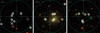 |
Fig. 4. Images of three HMCGs in SDSS. The inner circles show the minimum circle that encloses all the group members (ΘG), while the outer circles represent the radius of isolation (3ΘG). Galaxies with spectroscopic information and apparent magnitude r ≤ 17.77 are shown as solid lines, while photometric galaxies with r ≤ 17.77 are shown as dashed lines. Upward-pointing triangles are galaxies in the same magnitude range as the CG members; downward-pointing triangles are galaxies in the same redshift range as the CG; circles are galaxies outside the magnitude range of the CG. Light blue symbols are photometric galaxies considered as non-contaminating (see text), while the bright yellow symbols are potentially contaminating objects. Objects without symbols are either galaxies fainter than rlim = 17.77 or stars. Left: example of an HMCG without any potential sources of contamination (Group ID= 55 in Table D.1). Centre: CG with a non-contaminating galaxy within the disc of isolation whose photometric redshift is clearly outside the redshift range of the CG (Group ID= 210). Right: CG with two potential sources of contamination − one within the group radius and one in the isolation annulus− that we were not able to discard, while another photometric galaxy in the isolation annulus has been considered as non-contaminating (Group ID= 460). |
In addition, it is known that the SDSS spectroscopic survey suffers from incompleteness related to saturated bright galaxies and/or fibre collision for very close projected galaxy pairs. These issues could have an impact on the identification of CGs, mainly in the application of the population and isolation criteria. Therefore, we used the photometric information of galaxies extracted from the SDSS DR14 (Abolfathi et al. 2018) to search for potential galaxies that are in the surroundings of each identified CG and were neither detected in the spectroscopic survey nor incorporated by Tempel et al. (2017). In Appendix B, we describe the query used to retrieve galaxies without spectroscopy from SDSS DR14 Casjobs6.
From the sample of galaxies in SDSS without redshifts, we selected those that lie on the plane of sky within 3ΘG of the centre of each identified CG, and whose r model magnitudes are within a three-magnitude range from the brightest CG member galaxy (r ≤ rb + 3). This exercise provided us with a list of 303 objects without redshift information that might contaminate our sample of CGs. For these objects, we searched for alternative spectroscopic determinations in the literature using the NASA/IPAC Extragalactic Database (NED)7. We found that 63 of these galaxies had their redshifts already determined from different sources (see Table B.2). Objects misclassified as galaxies, as well as missing galaxies, might change the identification of CGs. Therefore, we corrected the parent catalogue of galaxies by discarding objects classified as PofGs and adding galaxies with available redshifts. The modified algorithm was run again on this corrected sample of 557 559 spectroscopic galaxies. We obtained a new sample of 462 HMCG in SDSS which constitutes our final catalogue (see Table 1).
We then again selected 290 photometric galaxies without redshift measurements that lie on the plane of the sky around the HMCGs in the same way as described above (angular proximity and magnitude range). We examined these objects to classify them either as potential sources of contamination or “non-contaminating” galaxies. This classification will be useful to determine whether our CGs fulfil the population and isolation criteria.
Among the 290 galaxies without SDSS spectroscopic red-shifts located in or close to HMCGs, we found that:
52 galaxies had spectroscopic redshifts as previously identified in Tempel et al. (2017);
53 other galaxies had photometric redshifts that are clearly discrepant with the HMCG median spectroscopic redshift (following Beck et al. 2016, galaxies with |zphot − zcm|/(1 + zcm) > 0.06 can be safely discarded as outliers);
104 of the other 185 galaxies were classified as non-contaminating objects, based on their photometric properties (see Appendix C for the criterion);
13 of the remaining 81 galaxies, after visual inspection via the SDSS DR14 Image List Tool, were determined to have been misclassified as galaxies by the SDSS pipeline;
the remaining 68 objects are potential sources of contamination.
In Fig. 4, we show three examples of regions around HMCGs. Pictures were taken from the SDSS DR14 Image Tool. Galaxy members are shown as upward-pointing triangles combined with downward-pointing triangles (stars) within or on top of the inner circle. The left picture shows an HMCG without any objects with unknown redshift within the group radius or the isolation annulus. The picture in the centre shows an example where two objects without redshift lie within the isolation radius (3ΘG), but one of the objects is outside the magnitude range of the group members (open dashed circle), while the other has a photometric redshift that is clearly discordant with the group and therefore is classified as a non-contaminating galaxy (upward-pointing dashed triangle); the other objects that can be seen in the same field without symbols are either galaxies fainter than the apparent magnitude limit of the SDSS spectroscopic sample or stars. Finally, the picture on the right shows a CG that is surrounded by three objects without known red-shifts and in the same magnitude range of the group members, one galaxy in the isolation annulus that has been classified as non-contaminating based on the method described in Appendix C (light blue dashed star), and two others (one inside the group radius and the other in the isolation annulus) that we were not able to discard as potential contaminants (bright yellow stars).
From the analysis of the potentially contaminating photometric objects from SDSS DR14, 18% are spectroscopically confirmed with external spectroscopy and were already included in our parent catalogue, 59% are clear outliers or misclassified objects, while roughly 23% are uncertain. Therefore, from our sample of 462 HMCGs, 406 of them can be considered clean (i.e. without sources of contamination), while 56 HMCGs need further information of galaxies in their surroundings in order to discard potential contamination sources.
In Appendix D, we present the new catalogue of HMCGs. Groups with potential contamination have not been discarded from our sample, but they are presented at the end of the tables with a flag that indicates the need for spectroscopic information of the potential sources of contamination (see Table C.2).
For the sake of comparison with the results found from the mock catalogues, we applied the classic algorithm to the extended and corrected sample of galaxies from SDSS, and we obtained a sample of 218 HCCGs (see Table 1). Similar to the results found in the mock catalogue, the modified algorithm was able to recover 95% of these groups, while it nearly doubles the number of CGs identified. Also, the classic algorithm misses almost half of the HMCGs due to discordant-velocity galaxies contaminating the isolation annulus. In Fig. 2, we show the boxplots obtained for the properties of CGs identified using both algorithms, where the samples are labelled Hickson classic (HC) and Hickson modified (HM). From this comparison, we observe trends similar to those in the samples obtained from the mock catalogue: the median values of dij, H0 tcr, ΘG, and μr are significantly higher with the modified method than with the classic method. Moreover, the analyses of completeness as a function of different properties produced the same results found for the mock samples. The completeness of the sample of CGs has therefore been improved with the new implementation of the algorithm.
4.3. Comparison with other compact group catalogues from SDSS
4.3.1. Compact group catalogues
A number of samples of CGs extracted from the SDSS have been presented in the literature. Particularly, McConnachie et al. (2009; hereafter McC09) identified CGs in projection in the SDSS data release 6 (DR6). It is worth mentioning that:
- i)
The identification in projection done by McC09 was performed up to magnitudes fainter than the SDSS spectroscopic limit (rlim = 17.77). One of their samples (catalogue A) is identified down to r ≤ 18, while the other (catalogue B) is for r ≤ 21.
- ii)
McC09 did not take into account the flux limit criterion (rb ≤ rlim − 3). Therefore, the isolation and population criteria were not strictly checked (as mentioned by McC09). Moreover, the lack of flux limit criterion could introduce an artificial correlation between group size and redshift.
- iii)
The CG identification was performed on a subsample of SDSS DR6 with only galaxies fainter than rinf = 14.5. This restriction led to a sample that misses low redshift CGs.
Later, Sohn et al. (2015) looked for velocity information from different sources for the galaxy members of McC09 CGs, and applied a velocity filter afterwards (SOHN15 CGs). In the best-case scenario, the resulting sample would be equivalent to the implementation of our classic algorithm.
Catalogues of compact groups from SDSS.
Another CG catalogue was extracted from SDSS DR12 by Sohn et al. (2016). They used a percolation algorithm with two fixed linking lengths, and looked for systems with high over-density contrast (small intergalaxy separations). They explicitly disregarded the isolation criterion, which could lead to a sample of small substructures within larger systems. This catalogue will be examined further in the following subsection.
In Table 2, we show the main characteristics of these CG samples extracted from different releases of SDSS8. The first six rows refer to the selection criteria of each sample. The middle rows have the number of CGs in each sample. Each row in this part of the table is obtained applying the restriction indicated in the first column and including the restrictions of the previous rows. Finally, the last four rows show the median of some properties of the samples of CGs resulting after applying all the restrictions to make the samples comparable. Given the small number of CGs in the restricted McC09 CG samples, these values cannot be included.
4.3.2. HMCGs vs SOHNCGs
As mentioned before, it is always difficult to compare samples of CGs identified by different authors given the inherent differences between the parent catalogues, the photometric bands, the algorithms, the definitions of what a compact group is, etc. However, we embraced this task and performed a detailed comparison between the new observational HMCG sample described in Sect. 4.2 and the CG sample identified by Sohn et al. (2016).
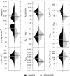 |
Fig. 5. Comparison of CG properties using asymmetric beanplots (Kampstra 2008). The black beans represent the density distributions for CGs identified with the modified algorithm (HMCGs), while grey distributions corresponds to the CGs that belong to the SOHNCGs sample. Both samples were restricted to perform a fair comparison (see text for details). Horizontal solid lines show the median values for each property distribution, while the horizontal dashed lines show the upper and lower limits of their corresponding 95% confidence intervals (Krzywinski & Altman 2014). This figure was made with R software (R Core Team 2013). |
Similar to our work, Sohn et al. have also used the catalogue of spectroscopic galaxies from the SDSS DR12 (Alam et al. 2015), but they complemented the survey themselves adding spectroscopic information extracted from other surveys such as Hwang et al. (2010) and NED, especially for bright galaxies (r < 14.5). Their final flux-limited galaxy sample includes 654 066 galaxies with magnitudes r < 17.77 in the redshift range 0.01 < z < 0.20.
Unlike us, the identification of CGs made by Sohn et al. (2016) was performed using a FoF algorithm similar to that used by Barton et al. (1996). Their FoF algorithm is based on two fixed linking lengths that restrict the projected physical spatial distance between galaxies (ΔD ≤ 50 kpc h−1) and the rest-frame line-of-sight velocity separation (ΔV ≤ 1000 km s−1) of every pair of neighbours. Moreover, in the spirit of the Hickson compact groups, they included the population and compactness criteria (N(Δr ≤ 3) ≥ 3 and μr ≤ 26 mag arcsec−2). However, they intentionally avoided applying any isolation criteria to their CGs. They presented a sample of 1588 CGs9. To perform a fair comparison with our sample, we needed to include several restrictions. To start with, we selected from their sample only those CGs with four or more galaxy members. The restricted sample comprises 312 CGs. Furthermore, we selected those groups that meet the flux limit criterion (rb ≤ rlim − 3) for which the population criterion has fully been checked, leading us to a smaller sample of 142 CGs. Finally, we applied the sky angular mask of the Tempel et al. (2017) catalogue to have the same angular coverage. All in all, the final sample comprises 109 groups (hereafter SOHNCG). By angularly cross-correlating this sample and our HMCGs, we found that 44% of the 109 SOHNCGs are included in our sample. The reasons why we were not able to recover the remaining 56% are discussed below.
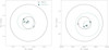 |
Fig. 6. Compact groups in common in the HMCGs and SOHNCGs samples. The HMCG galaxy members are represented as black squares, while the SOHNCG members are cyan triangles. The inner circle shows the minimum circle that encloses all the group members (ΘG), while the outer circle represents the disc of isolation (3ΘG). Each group centre is represented by a dot. Left panel: example of an embedded CG. The SOHNCG (Group ID = 600) lies inside the HMCG (Group ID = 53), while there are no galaxies within the disc of isolation of the SOHNCG. Right panel: example of a non-isolated subgroup (SOHNCG ID = 1115) that lies inside an HMCG (Group ID = 137). |
In addition, to compare both samples we also restricted our own sample to mimic the surface brightness limit imposed by Sohn et al. The two limits are different since they have kept the original limit from Hickson’s criterion in the R-band (μR < 26), while we have converted the limit to the r-band (μr < 26.33). With μr < 26.0, our sample decreases from 462 to 383 MHCGs. After making these samples comparable, we note that our HMCG sample is a factor of 3.5 larger than SOHNCG.
In Fig. 5, we compare the properties of these two samples of SDSS CGs. In this figure, we show asymmetric beanplots, i.e. the averaged density shape with a proper normalisation (see Kampstra 2008) for a given property, allowing us to make a direct comparison among the samples. Horizontal solid lines represent the median of the given property, while dashed lines represent their confidence intervals. From this comparison, we observe that the main difference is that SOHNCGs are smaller, producing ΘG, dij, μr, and H0 tcr distributions that are shifted towards lower values compared with the values obtained for our HMCG sample. These results could be related to the identification procedure: the small projected linking length used in the percolation algorithm by Sohn et al. (2016) leads to groups that are smaller in projection than those defined via Hickson-like finders. In addition, we observe that HMCGs show statistically brighter first-ranked galaxies and larger magnitude gaps between the two brightest galaxies (ΔM12) than their counterparts in SOHNCGs. Therefore, our sample is more dominated by its brightest galaxies.
Moreover, even though the median redshift for our HMCG sample is slightly shifted towards higher values (a difference of ∼0.005 in redshift or ∼1500 km s−1) compared with the corresponding SOHNCGs, this difference is not statistically significant (both lie within the 95% confidence interval of the other median) and the two density distributions are very similar. In comparison, Sohn et al. (2016) found that the red-shift distribution of their CG sample was roughly 9000 km s−1 lower (closer) than that of the sample that McConnachie et al. (2009) identified in the SDSS DR6 (with velocity filtering subsequently performed by Sohn et al. 2015). Sohn et al. (2016) attributed this difference to the isolation criterion incorporated by McConnachie et al. (2009). However, our classic and modified CGs have a median redshift similar to the Sohn et al. (2016) values. It should be noted that Sohn et al. (2016) performed a comparison between samples restricted to groups whose brightest galaxy was fainter than 14.5 because McConnachie et al. (2009) identified their CGs with this restriction. This omission of very bright galaxies might be a better explanation of the different redshift ranges of the McConnachie et al. (2009) and Sohn et al. (2016) CG samples than the inclusion or not of the isolation criterion.
Finally, to deepen our understanding of the differences found between our HMCGs and SOHNCGs, we first restricted the analysis to the 49 groups that are in common in both samples. Given that the matching has not been done on a one-by-one member basis, groups that are in common might still differ in their properties. In fact, we found that the differences mentioned above hold even for the samples that contain only the groups present in both samples. The HMCGs could be expected to be larger in projection because we intentionally selected them in this way: in the cases where there are galaxy associations that meet all the CG criteria inside larger associations that also fulfil all the criteria (embedded CGs), we preferred to keep the largest groups. To disentangle this issue, we then performed a member-by-member comparison and discovered that only seven cases (see left panel in Fig. 6) are embedded CGs in our sample. Also, we observe that there are 12 SOHNCGs that are subgroups inside our HMCGs that are not picked as CGs in our algorithm because the isolation is broken if the other galaxies are not included as part of the groups (see right panel of Fig. 6). Finally, there are nine groups where half of the galaxy members are not shared, even when the centres are very close, because the brightest galaxy is different and therefore the magnitude range in which the neighbours are considered differs. The remaining 21 groups are exactly the same. In the first two cases (which constitute ∼40% of the sample) the SOHNCGs are basically smaller substructures inside our groups which lead to the differences in sizes that we reported before. So, we conclude that the smaller sizes of SOHNCGs could be a consequence of the different definition of what a compact group is for each author more than a result of the algorithms themselves. On the other hand, analysing the 60 SOHNCGs that we were not able to recover, we found that we missed them because they failed our isolation criterion, while Sohn et al. (2016) did not apply this criterion.
5. Summary
The original definition of compact groups states that they are small, high density associations of bright galaxies that are relatively isolated in space (Hickson 1982). To identify such systems, groups must meet several criteria: limited population within a magnitude range, compactness, spatial isolation within a magnitude range, and velocity concordance of all of their galaxy members. While in principle the limiting values that can be adopted for each of the criteria are arbitrary, it is customary to adopt the definitions introduced by Hickson (1982) and Hickson et al. (1992). In this work, we followed these original ideas, and adopted the commonly used limits to present a new algorithm to identify CGs in redshift surveys.
The algorithm has been tested using a mock lightcone built from galaxies extracted from a recent semi-analytical model of galaxy formation (Henriques et al. 2015) run on top of the Millennium Simulation I rescaled to represent the cosmological model determined by the Plank cosmology. Given the methodology used to test the algorithm, the choice of a different semi-analytical model will not affect the results presented in this work.
To test the new algorithm we compared the resulting sample with that obtained using a previous version of the algorithm that had been used in the past to create and analyse samples of CGs (DíazGiménez & Mamon 2010; Díaz-Giménez et al. 2012; DíazGiménez & Zandivarez 2015; Taverna et al. 2016). We called the previous application of the algorithm classic, since it basically reproduces the steps followed by Hickson: it starts looking for CG in projection in the plane of the sky, and only when the projected sample is available does it check whether all the galaxy members have concordant radial velocities. Other authors have also followed these steps (Mendes de Oliveira & Hickson 1991; McConnachie et al. 2009; Sohn et al. 2015). The main disadvantage of the classic path is that when the algorithms involve the counting of galaxies in a magnitude range within a region of the projected sky, it may include many interlopers that lie in the line of sight in the background or foreground of the group itself. These inter-lopers will affect the population, as well as the isolation of the potential groups, and eventually some of the groups may be excluded from the projected sample. This could thus compromise the completeness of the resulting sample.
With the issue of the completeness in mind, we introduced a modified version of the algorithm. Instead of applying the velocity filter on a pre-selected projected sample of CGs, the velocity concordance is a requirement imposed as the galaxies are being included as galaxy members or neighbours.
As a result, we obtained modified samples that are roughly twice the size of the classic samples. We have shown that, compared to the classic version, the modified searching of CGs includes more groups towards the limit of the compactness criterion, with larger projected sizes, with fainter first-ranked galaxies, and with more similar two first-ranked galaxies. The incompleteness of the classic sample shows no dependence on distances to the groups.
Therefore, our modified algorithm helped us to improve the completeness of the samples of CGs. An interesting question now arises about the purity of the samples. Using the information in 3D real space from the simulation, and following DíazGiménez & Mamon (2010), we investigated the occurrence of chance alignments in our classic and modified CG samples. We found that the algorithm does not affect the fraction of CGs that are chance alignments of galaxies along the line of sight. It would have been desirable to diminish the fraction of chance alignment groups, but at least it has not increased even though we doubled the number of identified CGs. In a future work, we will investigate how to increase the fraction of physically dense compact groups (i.e. diminish the fraction of chance alignment groups) via observational constraints.
As a corollary of this study, we present a new CG catalogue identified on the observational spectroscopic galaxy sample compiled by Tempel et al. (2017) from the SDSS DR12. This CG catalogue comprises 462 systems. After performing visual and automatic inspections of the surroundings of each CG in the photometric SDSS sample, we determined that 406 CGs (∼88% of the sample) can certainly be considered isolated, while for the remaining 56 CGs we were not able to classify them as surely isolated, due to possible photometric contamination in their surrounding area caused by incompleteness inherent to the SDSS spectroscopic catalogue (saturation of bright galaxies and fibre collision). Further spectroscopic information is needed.
In addition, we performed a detailed comparison with the available sample of CGs identified by Sohn et al. (2016). The comparison between samples of CGs identified by different authors, algorithms, and criteria is never straightforward, and one has to be careful when extracting general conclusions about compact groups that could stand for CGs defined in one way but do not hold for a different sample. It is important to have larger samples of CGs identified in a unique homogeneous way, with well known selection criteria to obtain statistically reliable conclusions. With this aim either the sample of Sohn et al. (2016) and the sample introduced in this work achieve this goal, and to shed light on the properties of small peculiar galaxy systems, although the two samples differ in their definitions of what the authors understand by compact groups. Particularly, criteria regarding flux limit, isolation and embedded compact groups are key in determining the properties of the final sample of CGs.
The sample of 462 Hickson Modified Compact Groups (HMCGs) presented in this work has become the largest catalogue of CGs that satisfy all of Hickson’s original criteria: they are small, compact, and isolated associations of four or more concordant galaxies. This sample is available for the astronomical community in Tables D.1 and D.2 in this publication (see Appendix D for details).
The CG samples used in this work were downloaded from http://vizier.u-strasbg.fr/viz-bin/VizieR
Publicly available in VizieR as table http://vizier.u-strasbg.fr/viz-bin/VizieR-3?-source=J/ApJS/225/23
For galaxies with g−r colour less than 0 or greater than 1, we adopted the medians and the fit obtained for the whole sample of galaxies (yellow dots in Fig. A.1)
Acknowledgments
The authors would like to thank the referee, Dr. Gary Mamon, for his thoughtful analysis and suggestions that helped us to improve the original manuscript. The Millennium Simulation databases used in this paper and the web application providing online access to them were constructed as part of the activities of the German Astrophysical Virtual Observatory (GAVO). The observational data, which is a recompiled version of the publicly available SDSS data, was extracted from http://cosmodb.to.ee/. Funding for SDSS-III has been provided by the Alfred P. Sloan Foundation, the Participating Institutions, the National Science Foundation, and the US Department of Energy Office of Science. The SDSS-III website is http://www.sdss3.org/. SDSSIII is managed by the Astrophysical Research Consortium for the Participating Institutions of the SDSS-III Collaboration including the University of Arizona, the Brazilian Participation Group, Brookhaven National Laboratory, Carnegie Mellon University, University of Florida, the French Participation Group, the German Participation Group, Harvard University, the Instituto de Astrofisica de Canarias, the Michigan State/Notre Dame/JINA Participation Group, Johns Hopkins University, Lawrence Berkeley National Laboratory, Max Planck Institute for Astrophysics, Max Planck Institute for Extraterrestrial Physics, New Mexico State University, New York University, The Ohio State University, Pennsylvania State University, University of Portsmouth, Princeton University, the Spanish Participation Group, University of Tokyo, University of Utah, Vanderbilt University, University of Virginia, University of Washington, and Yale University. This research has made use of the NASA/IPAC Extragalactic Database (NED) which is operated by the Jet Propulsion Laboratory, California Institute of Technology, under contract with the National Aeronautics and Space Administration. This work has been partially supported by Consejo Nacional de Investigaciones Científicas y Técnicas de la República Argentina (CONICET) and the Secretaría de Ciencia y Tecnología de la Universidad de Córdoba (SeCyT).
References
- Abolfathi, B., Aguado, D. S., Aguilar, G., et al. 2018, ApJS, 235, 42 [NASA ADS] [CrossRef] [Google Scholar]
- Alam, S., Albareti, F. D., Allende Prieto, C., et al. 2015, ApJS, 219, 12 [NASA ADS] [CrossRef] [Google Scholar]
- Barton, E., Geller, M., Ramella, M., Marzke, R. O., & da Costa, L. N. 1996, AJ, 112, 871 [NASA ADS] [CrossRef] [Google Scholar]
- Beck, R., Dobos, L., Budavári, T., Szalay, A. S., & Csabai, I. 2016, MNRAS, 460, 1371 [NASA ADS] [CrossRef] [Google Scholar]
- Beers, T. C., Flynn, K., & Gebhardt, K. 1990, AJ, 100, 32 [NASA ADS] [CrossRef] [Google Scholar]
- Bertone, S., De Lucia, G., & Thomas, P. A. 2007, MNRAS, 379, 1143 [NASA ADS] [CrossRef] [Google Scholar]
- Chilingarian, I. V., & Zolotukhin, I. Y. 2012, MNRAS, 419, 1727 [NASA ADS] [CrossRef] [Google Scholar]
- Colless, M., Dalton, G., Maddox, S., et al. 2001, MNRAS, 328, 1039 [NASA ADS] [CrossRef] [Google Scholar]
- Colless, M., Peterson, B. A., & Jackson, C. 2003, ArXiv e-prints [astro-ph/0306581] [Google Scholar]
- Corwin, H. G., Jr,, Buta, R. J., & de Vaucouleurs, G. 1994, AJ, 108, 2128 [NASA ADS] [CrossRef] [Google Scholar]
- de Vaucouleurs, G., de Vaucouleurs, A., & Corwin, H. G. 1991, Third Reference Catalogue of Bright Galaxies (New York, NY: Springer) [Google Scholar]
- Díaz-Giménez, E., & Mamon, G. A. 2010, MNRAS, 409, 1227 [NASA ADS] [CrossRef] [Google Scholar]
- Díaz-Giménez, E., & Zandivarez, A. 2015, A&A, 578, A61 [NASA ADS] [CrossRef] [EDP Sciences] [Google Scholar]
- Díaz-Giménez, E., Mamon, G. A., Pacheco, M., de Mens Oliveira, C., & Alonso, M. V. 2012, MNRAS, 426, 296 [NASA ADS] [CrossRef] [Google Scholar]
- Doi, M., Tanaka, M., Fukugita, M., et al. 2010, AJ, 139, 1628 [NASA ADS] [CrossRef] [Google Scholar]
- Eisenstein, D. J., Weinberg, D. H., Agol, E., et al. 2011, AJ, 142, 72 [Google Scholar]
- Focardi, P., & Kelm, B. 2002, A&A, 391, 35 [NASA ADS] [CrossRef] [EDP Sciences] [Google Scholar]
- Henriques, B. M. B., White, S. D. M., Thomas, P. A., et al. 2015, MNRAS, 451, 2663 [NASA ADS] [CrossRef] [Google Scholar]
- Hickson, P. 1982, ApJ, 255, 382 [NASA ADS] [CrossRef] [Google Scholar]
- Hickson, P., de Mens Oliveira, C., Huchra, J. P., & Palumbo, G. G. 1992, ApJ, 399, 353 [NASA ADS] [CrossRef] [EDP Sciences] [MathSciNet] [PubMed] [Google Scholar]
- Huchra, J. P., Macri, L. M., Masters, K. L., et al. 2012, ApJS, 199, 26 [NASA ADS] [CrossRef] [Google Scholar]
- Hwang, H. S., Elbaz, D., Lee, J. C., et al. 2010, A&A, 522, A33 [NASA ADS] [CrossRef] [EDP Sciences] [Google Scholar]
- Iovino, A. 2002, AJ, 124, 2471 [NASA ADS] [CrossRef] [Google Scholar]
- Jarrett, T. H., Chester, T., Cutri, R., Schneider, S. E., & Huchra, J. P. 2003, AJ, 125, 525 [NASA ADS] [CrossRef] [Google Scholar]
- Kampstra, P. 2008, J. Stat. Softw. Code Snippets, 28, 1 [Google Scholar]
- Krzywinski, M., & Altman, N. 2014, Nat. Methods, 11, 119 [CrossRef] [Google Scholar]
- Lange, R., Driver, S. P., Robotham, A. S. G., et al. 2015, MNRAS, 447, 2603 [NASA ADS] [CrossRef] [Google Scholar]
- Lee, B. C., Allam, S. S., Tucker, D. L., et al. 2004, AJ, 127, 1811 [NASA ADS] [CrossRef] [Google Scholar]
- Mamon, G. A. 1986, ApJ, 307, 426 [NASA ADS] [CrossRef] [Google Scholar]
- Mamon, G. A. 1990, in NASA Conf. Pub., eds. J. W. Sulentic, W. C. Keel, & C. M. Telesco, 3098 [Google Scholar]
- McConnachie, A. W., Ellison, S. L., & Patton, D. R. 2008, MNRAS, 387, 1281 [NASA ADS] [CrossRef] [Google Scholar]
- McConnachie, A. W., Patton, D. R., Ellison, S. L., & Simard, L. 2009, MNRAS, 395, 255 [NASA ADS] [CrossRef] [Google Scholar]
- McGill, R., Tukey, J. W., & Larsen, W. A. 1978, The American Statistician, 32, 12 [Google Scholar]
- Mens de Oliveira, C., & Hickson, P. 1991, ApJ, 380, 30 [NASA ADS] [CrossRef] [Google Scholar]
- Planck Collaboration XVI. 2014, A&A, 571, A16 [NASA ADS] [CrossRef] [EDP Sciences] [Google Scholar]
- Prandoni, I., Iovino, A., & MacGillivray, H. T. 1994, AJ, 107, 1235 [NASA ADS] [CrossRef] [Google Scholar]
- R Core Team 2013, R: A Language and Environment for Statistical Computing (Vienna, Austria: R Foundation for Statistical Computing) [Google Scholar]
- Scrucca, L., Fop, M., Murphy, T. B., & Raftery, A. E. 2017, The R Journal, 8, 205 [Google Scholar]
- Skrutskie, M. F., Cutri, R. M., Stiening, R., et al. 2006, AJ, 131, 1163 [NASA ADS] [CrossRef] [Google Scholar]
- Sohn, J., Hwang, H. S., Geller, M. J., et al. 2015, J. Korean Astron. Soc., 48, 381 [NASA ADS] [CrossRef] [Google Scholar]
- Sohn, J., Geller, M. J., Hwang, H. S., Zahid, H. J., & Lee, M. G. 2016, ApJS, 225, 23 [NASA ADS] [CrossRef] [Google Scholar]
- Springel, V., White, S. D. M., Jenkins, A., et al. 2005, Nature, 435, 629 [NASA ADS] [CrossRef] [PubMed] [Google Scholar]
- Taverna, A., Díaz-Giménez, E., Zandivarez, A., Joray, F., & Kanagusuku, M. J. 2016, MNRAS, 461, 1539 [NASA ADS] [CrossRef] [Google Scholar]
- Tempel, E., Tuvikene, T., Kipper, R., & Libeskind, N. I. 2017, A&A, 602, A100 [NASA ADS] [CrossRef] [EDP Sciences] [Google Scholar]
- Zandivarez, A., Domínguez, M. J. L., Ragone, C. J., Muriel, H., & Martínez, H. J. 2003, MNRAS, 340, 1400 [NASA ADS] [CrossRef] [Google Scholar]
- Zandivarez, A., Díaz-Giménez, E., Mendes de Oliveira, C., et al. 2014a, A&A, 561, A71 [NASA ADS] [CrossRef] [EDP Sciences] [Google Scholar]
- Zandivarez, A., Díaz-Giménez, E., de Mens Oliveira, C. & Gubolin, H. 2014b, A&A, 572, A68 [NASA ADS] [CrossRef] [EDP Sciences] [Google Scholar]
Appendix A: K-decorrection
To obtain the observer-frame magnitudes for galaxies in the lightcones, one has to “k-decorrect” the rest-frame magnitudes provided by the SAMs. For this purpose, we developed an iterative process based on observational data.
First, using the observer-frame magnitudes and colours of galaxies in the SDSS DR14 we computed the k-corrections for those galaxies using the prescriptions of Chilingarian & Zolotukhin (2012) which, in addition to red-shifts, use the observer-frame magnitude and colours as inputs. Figure A.1 shows the k-corrections in the r-band as a function of redshift. Once the k-corrections are obtained, we computed the rest-frame colours of galaxies, and split the sample into several colour ranges. For each rest-frame colour range, we computed the median values of k-corrections per bin of redshift. We considered these median values as a good approximation up to a limiting distance (z = 0.25 in Fig. A.1). For larger values of redshifts, we computed a linear fit for each rest-frame colour range. For galaxy colours outside the ranges defined in the figure (i.e. g − r ≤ 0 OR g − r > 1), we adopt the values corresponding to the total sample of galaxies (grey stars in the figure).
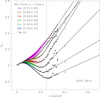 |
Fig. A.1. k-correction vs redshift for galaxies in the SDSS DR14 split by rest-frame colours (see inset labels). k-corrections are computed using Chilingarian & Zolotukhin 2012. Black dots are the median values of the k-corrections for a given redshift bin for each colour range. Grey stars are the medians for the whole sample of galaxies regardless their colour. Black straight lines are the linear fits to the dots with redshift greater than 0.25 (vertical solid line). |
In this way, using the observational fits, we are able to obtain a first approximation to the k-corrections of galaxies when we only have access to their rest-frame colours and red-shifts: for galaxies at redshifts lower than z = 0.25, we use linear interpolations between the median values of k-corrections per bin of redshifts (black dots in Fig. A.1). For higher red-shifts, we used the linear fits obtained from the data10. Then, we compute the observer-frame colours and use them as inputs in the original Chilingarian & Zolotukhin prescriptions. With these k-corrections, we then compute new observer-frame magnitudes and iterate into the Chilingarian & Zolotukhin prescriptions one more time to compute final k-corrections to k-decorrect the original rest-frame magnitudes and estimate the final observer-frame magnitudes.
We tested this iterative procedure using SDSS DR14 galaxies. Starting with the observer-frame magnitudes from the catalogue, we obtained the k-corrections via Chilingarian & Zolotukhin and computed their rest-frame magnitudes. These rest-frame magnitudes are used as inputs in our iterative process in which the observer-frame magnitudes are estimated. Comparing the observed observer-frame magnitudes with the estimated observer-frame magnitudes, we obtained that the 99th percentile of the difference of |robserved − rcomputed| is 0.009 mag, which indicates the success of the method.
The Fortran subroutine used to k-decorrect magnitudes and obtain observer-frame magnitudes in mock catalogues starting from rest-frame magnitudes is publicly available at the author’s institute web page11. The code can also be used for the K2MASS- band which has been tested on galaxies from the 2MRS catalogue (Huchra et al. 2012).
Appendix B: Tables of galaxies
In this appendix we provide further information about galaxies used in this work:
In Table B.1 we quote the SDSS object identification number (ObjID) of 21 galaxies in the Tempel et al. (2017) catalogue that were visually classified as part of a galaxy (PofG).
-
We selected galaxies from SDSS DR14 for which the SDSS-III imaging pipeline has declared the photometry clean12. The query is quoted below:
1 SELECT px.objlD,px.ra,px.dec,px. modelMag_u,px.modelMag_g,px. modelMag_r,px.modelMag_i,px. modelMag_z,px.modelMagErr_u,px. modelMagErr_g,px.modelMagErr_r,px. modelMagErr_i,px.modelMagErr_z,px. extinction_u,px.extinction_g,px. extinctions_r,px.extinction_i,px. extinction_z,pxx.petroRad_r,pxx. petroRadErr_r,pxx.petroR50_r,pxx. petroR50Err_r,pxx.petroR90_r,pxx. petroR90Err_r,pz.z,pz.zErr,pz. nnCount,pz.photoErrorClass
2 FROM GalaxyTag as px,
3 Photoz as pz,
4 PhotoObjAll as pxx
5 WHERE px.modelMag.r<=17.77
6 AND px.type=3
7 AND px.mode=l
8 AND ((px.flags_r & 0x10000000) !=0)
9 AND ((px.flags_r & 0x8100000c00a0)=0)
10 AND ((px.flags_r & 0x400000000000)=0)
11 OR (px.psfmagerr_r<=0.2))
12 AND ((px.flags_r & 0x100000000000)=0)
13 OR (px.flags_r & 0xl000)=0)
14 AND px.ObjID=pz.ObjID
15 AND pxx.ObjID=px.ObjID
16 AND px.spec0bjID=0
Table B.1.Galaxies in the Tempel et al. (2017) catalogue around potential compact groups that were visually classified as Part of a Galaxy (PofG).
The methods used to calculate the photometric redshift estimates retrieved with this query are described in Beck et al. (2016).
-
From the sample of galaxies without redshifts described in the previous item, we selected those galaxies that satisfy r > 0, g − r < 3. Magnitudes were corrected for extinction and transformed to the AB system (Doi et al. 2010). Some of these galaxies were found to have their redshifts available in the NED. In Table B.2 we quote the redshifts found for the photometric galaxies around CG candidates. We corrected the redshifts to the CMB rest frame using the standard equation
![$$ {z_{{{\rm CMB}}}} = {z_{{\rm{NED}}}} + {z_a}[\sin b\sin {b_a} + \cos b\cos {b_a}\cos ({l_a} - l)] $$](/articles/aa/full_html/2018/10/aa33329-18/aa33329-18-eq7.gif) (B.1)
(B.1)where l and b are the galactic coordinates, la = 264.14°, ba = 48.26°, and za = 371.0/c (subscript a is the abbreviation of apex) and c is the velocity of light in vacuum in km s−1.
Appendix C: Non-contaminating galaxies
In this appendix, we focus on the 185 photometric galaxies considered as potential sources of contamination of HMCGs in Sect. 4.2. We compared the photometric properties of these galaxies with those of the spectroscopic galaxies around the same HMCGs that they might be contaminating.
For each group with a potential contaminating galaxy, we selected spectroscopic galaxies from the SDSS DR14 that are:
inside a circle of 5 degrees radius from the HMCG centre,
within a 3 mag range from the HMCG first-ranked galaxy,
and within 1000 km s−1 of the HMCG median radial velocity.
Redshift corrected to the CMB rest frame for 63 photometric galaxies in the SDSS DR14 extracted from the NASA/IPAC Extragalactic Database (NED).
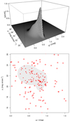 |
Fig. C.1. Upper plot: perspective plot of the bivariate density estimate in the surface brightness vs colour plane for the spectroscopic galaxies in the SDSS DR14 that are in the same redshift and magnitude ranges as those HMCGs that contain potentially contaminating photometric galaxies. Lower plot: grey area encloses 95% of the spectroscopic galaxies. Red filled dots are photometric galaxies in the same magnitude range of their host CGs, and that are considered potential sources of contamination (inside the grey region), while red open dots are galaxies classified as non-contaminating objects (outside the grey region)(see text for details). |
Mclust best fitted parameters obtained for the bivariate density estimate from four Gaussian functions in the surface brightness − colour plane.
Galaxies in the SDSS DR14 photometric catalogue around compact groups that are potential sources of contamination.
We measured the surface brightnesses (μr) and observer-frame colours (g−r) of each spectroscopic galaxy and of the potentially contaminating galaxies. The surface brightness of each galaxy was computed using the Petrosian radius provided by the SDSS pipeline. After analysing the surface brightness − colour relation, we used the Mclust package (Scrucca et al. 2017) of R software to perform a density estimation based on finite Gaussian mixture modelling. From its application to our data in the surface brightness − colour plane, we observed that, according to the Bayesian Information Criterion, a proper density representation can be obtained using a mixture of four Gaussian functions for a model with ellipsoidal distribution that allows variable volume, shape, and orientation. The best fitted parameters for the obtained Gaussian mixture modelling are quoted in Table C.1, while the perspective plot of the resulting surface density is shown in the upper panel of Fig. C.1.
Using this surface density, we defined the isodensity contour that enclosed 95% of the spectroscopic galaxies in the surface brightness − colour plane. This region is represented as the grey. shaded area in the lower panel of Fig. C.1. We also show the scatter plot for the potential sources of contamination (red dots) Photometric galaxies lying outside the grey region are considered non-contaminating galaxies (empty red dots). This criterion allowed us to discard 104 galaxies.
Finally, as described in Sect. 4.2, after a visual inspection of the remaining 81 objects, we confirm that 13 were actually objects misclassified as galaxies by the SDSS pipeline. Therefore, only 68 galaxies are kept as potential sources of contamination. The SDSS object identification numbers of these 68 galaxies are quoted in Table C.2.
Appendix D: New CG catalogue in the SDSS
In this appendix we present the tables of HMCGs identified in the SDSS. In Table D.1 we show the content for the table containing 462 HMCGs, while Table D.2 shows the content for the table that contains the information for the 2070 galaxy members.
Compact groups identified in the SDSS DR12 using the modified algorithm.
Galaxy members of compact groups identified in SDSS DR12 using the modified algorithm.
All Tables
Galaxies in the Tempel et al. (2017) catalogue around potential compact groups that were visually classified as Part of a Galaxy (PofG).
Redshift corrected to the CMB rest frame for 63 photometric galaxies in the SDSS DR14 extracted from the NASA/IPAC Extragalactic Database (NED).
Mclust best fitted parameters obtained for the bivariate density estimate from four Gaussian functions in the surface brightness − colour plane.
Galaxies in the SDSS DR14 photometric catalogue around compact groups that are potential sources of contamination.
Galaxy members of compact groups identified in SDSS DR12 using the modified algorithm.
All Figures
|
Fig. 1. Flow charts showing the automatic implementation of the Hickson’s criteria to identify CGs. On the left the flow chart shows the classic algorithm, while on the right the modified algorithm is shown. |
| In the text | |
|
Fig. 2. Boxplot diagrams of CG properties for groups identified using the classic and the modified algorithm. The notches (waists) in the boxes indicate ∼95 % confidence intervals for the medians, while the widths are proportional to the square roots of the number of objects in each sample (R Core Team 2013). The boxplot diagrams on the left side in each panel are the samples obtained using the classic and the modified algorithms in the mock catalogue (mHC and mHM), while those at the right side show the results for the samples obtained applying both algorithms on the SDSS catalogue (HC and HM). |
| In the text | |
|
Fig. 3. Ratio of the classic to the modified distributions for a given property. Shaded areas correspond to the errors computed using the error propagation formula for the ratio (each number in the ratio has a Poisson error). |
| In the text | |
|
Fig. 4. Images of three HMCGs in SDSS. The inner circles show the minimum circle that encloses all the group members (ΘG), while the outer circles represent the radius of isolation (3ΘG). Galaxies with spectroscopic information and apparent magnitude r ≤ 17.77 are shown as solid lines, while photometric galaxies with r ≤ 17.77 are shown as dashed lines. Upward-pointing triangles are galaxies in the same magnitude range as the CG members; downward-pointing triangles are galaxies in the same redshift range as the CG; circles are galaxies outside the magnitude range of the CG. Light blue symbols are photometric galaxies considered as non-contaminating (see text), while the bright yellow symbols are potentially contaminating objects. Objects without symbols are either galaxies fainter than rlim = 17.77 or stars. Left: example of an HMCG without any potential sources of contamination (Group ID= 55 in Table D.1). Centre: CG with a non-contaminating galaxy within the disc of isolation whose photometric redshift is clearly outside the redshift range of the CG (Group ID= 210). Right: CG with two potential sources of contamination − one within the group radius and one in the isolation annulus− that we were not able to discard, while another photometric galaxy in the isolation annulus has been considered as non-contaminating (Group ID= 460). |
| In the text | |
|
Fig. 5. Comparison of CG properties using asymmetric beanplots (Kampstra 2008). The black beans represent the density distributions for CGs identified with the modified algorithm (HMCGs), while grey distributions corresponds to the CGs that belong to the SOHNCGs sample. Both samples were restricted to perform a fair comparison (see text for details). Horizontal solid lines show the median values for each property distribution, while the horizontal dashed lines show the upper and lower limits of their corresponding 95% confidence intervals (Krzywinski & Altman 2014). This figure was made with R software (R Core Team 2013). |
| In the text | |
|
Fig. 6. Compact groups in common in the HMCGs and SOHNCGs samples. The HMCG galaxy members are represented as black squares, while the SOHNCG members are cyan triangles. The inner circle shows the minimum circle that encloses all the group members (ΘG), while the outer circle represents the disc of isolation (3ΘG). Each group centre is represented by a dot. Left panel: example of an embedded CG. The SOHNCG (Group ID = 600) lies inside the HMCG (Group ID = 53), while there are no galaxies within the disc of isolation of the SOHNCG. Right panel: example of a non-isolated subgroup (SOHNCG ID = 1115) that lies inside an HMCG (Group ID = 137). |
| In the text | |
|
Fig. A.1. k-correction vs redshift for galaxies in the SDSS DR14 split by rest-frame colours (see inset labels). k-corrections are computed using Chilingarian & Zolotukhin 2012. Black dots are the median values of the k-corrections for a given redshift bin for each colour range. Grey stars are the medians for the whole sample of galaxies regardless their colour. Black straight lines are the linear fits to the dots with redshift greater than 0.25 (vertical solid line). |
| In the text | |
|
Fig. C.1. Upper plot: perspective plot of the bivariate density estimate in the surface brightness vs colour plane for the spectroscopic galaxies in the SDSS DR14 that are in the same redshift and magnitude ranges as those HMCGs that contain potentially contaminating photometric galaxies. Lower plot: grey area encloses 95% of the spectroscopic galaxies. Red filled dots are photometric galaxies in the same magnitude range of their host CGs, and that are considered potential sources of contamination (inside the grey region), while red open dots are galaxies classified as non-contaminating objects (outside the grey region)(see text for details). |
| In the text | |
Current usage metrics show cumulative count of Article Views (full-text article views including HTML views, PDF and ePub downloads, according to the available data) and Abstracts Views on Vision4Press platform.
Data correspond to usage on the plateform after 2015. The current usage metrics is available 48-96 hours after online publication and is updated daily on week days.
Initial download of the metrics may take a while.