| Issue |
A&A
Volume 618, October 2018
|
|
|---|---|---|
| Article Number | A26 | |
| Number of page(s) | 11 | |
| Section | The Sun | |
| DOI | https://doi.org/10.1051/0004-6361/201732432 | |
| Published online | 09 October 2018 | |
Structure of the heliosheath from HSTOF energetic neutral atoms measurements
1
Space Research Centre, Polish Academy of Sciences, Bartycka 18A, 00-716 Warsaw, Poland
e-mail: ace@cbk.waw.pl
2
Max-Planck-Institut fuer Sonnensystemforschung, Justus-von-Liebig Weg 3, 37077 Göttingen, Germany
3
Physics Department, University of Arizona, Tucson, AZ, 85721 USA
Received:
7
December
2017
Accepted:
2
July
2018
Context. From the year 1996 until now, High energy Suprathermal Time Of Flight sensor (HSTOF) on board Solar and Heliospheric Observatory (SOHO) has been measuring the heliospheric energetic neutral atoms (ENA) flux between ±17° from the ecliptic plane. At present it is the only ENA instrument with the energy range within that of Voyager LECP energetic ion measurements. The energetic ion density and thickness of the inner heliosheath along the Voyager 1 trajectory are now known, and the ENA flux in the HSTOF energy range coming from the Voyager 1 direction may be estimated.
Aims. We use HSTOF ENA data and Voyager 1 energetic ion spectrum to compare the regions of the heliosheath observed by HSTOF and Voyager 1.
Methods. We compared the HSTOF ENA flux data from the forward and flank sectors of the heliosphere observed in various time periods between the years 1996 and 2010 and calculated the predicted ENA flux from the Voyager 1 direction using the Voyager 1 LECP energetic ion spectrum and including the contributions of charge exchange with both neutral H and He atoms.
Results. The ratio between the HSTOF ENA flux from the ecliptic longitude sector 210−300° (the LISM apex sector) for the period 1996−1997 to the estimated ENA flux from the Voyager 1 direction is ∼1.3, but decreases to ∼0.6 for the period 1996−2005 and ∼0.3 for 1998−2006. For the flank longitude sectors (120−210° and 300−30°), the ratio also tends to decrease with time from ∼0.6 for 1996−2005 to ∼0.2 for 2008−2010. We discuss implications of these results for the energetic ion distribution in the heliosheath and the structure of the heliosphere.
Key words: Sun: heliosphere / solar wind / interplanetary medium
© ESO 2018
1. Introduction
Launched in 1995, High energy Suprathermal Time Of Flight sensor (HSTOF) on board Solar and Heliospheric Observatory (SOHO) was the first instrument dedicated to observations of the heliospheric energetic neutral atoms (ENA). After the September 15, 2017 demise of the spacecraft Cassini with Ion and Neutral Camera (INCA) on board, HSTOF is presently the only ENA instrument with the energy range overlapping with Voyager Low Energy Charged Particle (LECP) measurements of the energetic ion fluxes in the heliosheath.
A comparison of the ion flux intensity from Voyager data with the measured ENA flux can be used to estimate, by means of the approximate relation JENA(E) = Jion(E)σcxnHL, the value of the product nHL of the neutral hydrogen density nH and the thickness L of the source region (presumably, the inner heliosheath). From this result, the thickness L can be estimated, assuming a value for nH in the source region based on other observations and theoretical models.
The HSTOF observation region is restricted in ecliptic latitude to the belt within ±17° from the ecliptic plane. The Voyager 1 (ecliptic latitude 34.7° in 2005) and Voyager 2 (latitude −29.8° in 2005) trajectories are outside this region. Combining, nevertheless, the HSTOF ENA and the Voyager LECP ion data, the thickness of the inner heliosheath was estimated to be 21 ± 6 AU for the Voyager 1 direction and 28 ± 8 AU for the Voyager 2 direction (Hsieh et al. 2010), assuming nH = 0.1 cm−3 and neglecting the contribution from the charge exchange with the neutral helium background.
With these assumptions, Voyager 1 was predicted (Hsieh et al. 2010) to cross the heliopause in late 2010 at the distance of ∼115 AU from the Sun. A prediction of a short distance to the heliopause was at the time unique and not supported by model simulations.
In 2012 Voyager 1 crossed the so-called heliocliff: a sharp drop (to a level consistent with that expected in the interstellar medium) of the flux intensity of the low energy part of the energetic ion spectrum (Stone et al. 2013; Webber & McDonald 2013; Krimigis et al. 2013). Assuming that the heliocliff is identical with the heliopause, the thickness of the inner heliosheath along the Voyager 1 direction was approximately determined by subtracting the distance to the termination shock (94 AU) from the distance to the cliff (122 AU) to give 28 AU, which is higher, by 7 AU, than the result based on HSTOF ENA given in Hsieh et al. (2010).
As shown below (Sect. 3), taking the contribution from charge exchange of protons with the neutral helium into account, significantly decreases the estimation based on HSTOF and makes this difference even larger, exceeding the statistical (1σ) error of the HSTOF measurements.
In the following we use HSTOF ENA data and Voyager 1 observations in the heliosheath to compare the regions of the inner heliosheath observed by Voyager 1 and by HSTOF. We present the HSTOF hydrogen and helium ENA fluxes averaged over selected time intervals between the years 1996 and 2010.
Throughout this paper, we use a simple fit (Hsieh et al. 2010) to the Voyager 1 LECP ion spectrum in the inner heliosheath (i.e., between the termination shock and heliopause) Voyager 1 LECP observations refer to the ions with Z ≥ 1 and energies > 40 keV. The fit covers the period between 2004 DOY 249 and 2009 DOY 105. The ion flux measured by Voyager 1 was fairly steady over this period except for transient effects. After the year 2009 the flux started to decrease (Dialynas et al. 2017).
From Voyager 1 LECP measurements between the termination shock and heliopause, we derive the ENA flux (in the HSTOF energy range) from the Voyager 1 direction. We take into account the charge exchange of protons with both hydrogen and helium, using best available estimations of the ambient hydrogen and helium densities. The result is higher than the ENA flux measured by HSTOF in the ecliptic longitude sectors corresponding to the flanks of the heliosphere (see Fig. 1). We conclude that the column density of the energetic ions along the Voyager 1 direction (observation period from 2004 DOY 249 to 2009 DOY 105) is higher than the average column density in the flank sectors of the HSTOF ENA source region (observation period 1996−2010).
The ENA observations by HSTOF are presented in Sect. 2. In Sect. 3 we compare the HSTOF and Voyager 1 observation regions in the inner heliosheath using the ENA measurements by HSTOF and the energetic ion measurements by Voyager 1. Section 4 contains a discussion of selected topics related to the observations by HSTOF: the ENA flux maximum from the heliotail direction, the difference between the ENA fluxes from two flanks, and the limits on the timescales of ENA flux variations in the HSTOF observation sectors. The conclusions are presented in Sect. 5.
2. ENA observations by HSTOF
The instrument HSTOF (Hovestadt et al. 1995), which is a part of the experiment Charge, Element and Isotope Analysis System (CELIAS) on board SOHO, measures hydrogen (58−88 keV) and helium (28−58 keV n−1) ENA fluxes within ±17° from the ecliptic.
Because of low ENA flux, in analyzing the HSTOF data it is necessary to use averages over large enough time periods and ecliptic longitude ranges. Figure 1 shows the two ecliptic longitude sectors used in the early work (extended forward and the tail) and the four sectors used in more recent studies (Hilchenbach et al. 2006; Hsieh et al. 2010; Czechowski et al. 2008; Czechowski et al. 2012).
Until the year 2003, the whole range of the ecliptic longitude was scanned yearly. After the year 2005, only the flank sectors are accessible to observations.
Voyager 1 and Voyager 2 trajectories through the heliosheath are outside the ecliptic latitude limits of the HSTOF observation region (by about 18° to the north for Voyager 1 and to the south for Voyager 2), while their longitudes are inside the forward ecliptic longitude sector of HSTOF. The forward sector is therefore the closest to the Voyager 1 and Voyager 2 observation regions.
The ENA observations by HSTOF are only possible during quiet times when the ambient energetic ion fluxes are low (Hilchenbach et al. 1998; Hilchenbach et al. 2001). In consequence, the HSTOF ENA data come predominantly from the periods near the solar minima: the years 1996−1997 (during the year 1998 the contact with SOHO was lost for a time) and the years 2008−2010 (for which the forward and tail sectors cannot be observed). The ENA fluxes measured during the latter period are significantly lower than for the years 1996−1997 (Czechowski et al. 2012). Cross calibration of the instrument ion channels with Advanced Composition Explorer (ACE) data was performed to check for a possible instrumental effect (Czechowski et al. 2012). The result was similar to previous cross calibration, concerning the comparison of ACE and HSTOF energetic ion flux and the HSTOF response for the various energy range intervals.
The helium ENA data were recently re-analyzed using corrected background (Hilchenbach et al. 2012) and only those are used in the present study. The directional dependence of the ENA flux measured by HSTOF differs from the observations by other instruments. In both H and He HSTOF ENA data the flux maximum is situated close to the anti-apex direction of the interstellar medium (ISM) flow (Figs. 2 and 3). A possible explanation is discussed in Sect. 4.1.
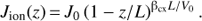
A large part of the HSTOF data comes from the times before the year 2004, when Voyager 1 entered the heliosheath (Stone et al. 2005; Decker et al. 2005). The question of possible time dependence of the HSTOF ENA flux data is therefore important. The yearly averages of the HSTOF ENA flux measurements between the years 1996 and 2005 for the forward sector are given in Hilchenbach et al. (2006), but the uncertainties are too large to confirm the time dependence reliably. We used these data to construct the average over the periods 1996−1997 and 1998−2005 presented in Fig. 2, in addition to the averages for the extended forward sector (which includes also the flanks). The results show that the flux in the years 1996−1997 is higher than in the 1998−2005 period for the cases of the forward sector, extended forward sector, and tail sector.
We note that the period 1996−1997 has a larger percentage of quiet times than the 1998−2003 period. This could be thought to indicate a positive correlation between the estimated flux and observing conditions. On the other hand, the data for the period 2008−2010 (the flanks) have a similarly large percentage of quiet times, but do not have a particularly large flux value.
In the case of flank sectors, the 1996−2005 hydrogen flux for the right flank is significantly higher than for the 2006−2008 and 2008−2010 time periods, but the decrease is much smaller for the left flank (Fig. 2). Comparing the averages over the periods 1996−2005 and 1996−2010 for the helium ENA flux (Fig. 3) suggests a similar behavior.
The decrease of the ENA flux intensity with time may be correlated with the decrease in the solar wind flux (Fig. 4) by a factor of 2 between the years 1992 and 2010 (Sokół et al. 2013, Fig. 3; McComas et al. 2013, Fig. 2). There are three periods of relatively fast falloff, each by a similar relative amount (28−29% of the before–after average), commencing in the years 1992, 1997, and 2005. The solar wind falloffs starting in 1997 and in 2005 occur close to the periods of apparent decreases in the ENA flux shown in Figs. 2 and 3. However, since these ENA data are mostly long-term averages, we cannot use them to resolve the real time dependence. The temporal variation of the ENA flux is discussed in Sects. 4.3 and 4.4.
Instead of averages over the whole energy range, one may consider the ENA flux values for the lowest energy bins. In the case of hydrogen, this choice does not affect the time dependence, but for the case of helium, the time dependence of the flux is then much reduced and becomes statistically insignificant in each of the flank sectors (see discussion in Czechowski et al. 2012).
After the year 2005 the HSTOF ENA data do not include the forward and heliotail sectors. If the hydrogen ENA flux decrease seen in the flank sectors also occurs in the forward ecliptic longitude sector, the comparison between the HSTOF ENA measurements and Voyager ion flux measurements in the heliosheath would be significantly affected. In particular, the use of the HSTOF ENA flux average over the years 1996−2005, as carried out in Hsieh et al. (2010), would lead to an overestimate of the ENA flux during most of the Voyager 1 observation period in the inner heliosheath. The thickness of the heliosheath obtained by Hsieh et al. (2010) would then also be overestimated.
We note that, in the 1996−2005 time period, the hydrogen and helium fluxes in the right flank sector are higher than those in the left flank. This can be qualitatively understood in terms of the geometry of the heliosphere (see Sect. 4.2).
 |
Fig. 1. Ecliptic longitude sectors used for presenting HSTOF data. The four sectors shown on the left are used in the recent studies. The forward sector, which includes the inflow direction of the ISM (eliptic longitude 255°), is also called the “apex”, or the “nose sector”. Early work employed two sectors with the extended “forward sector” that also included the flanks (see right side of figure). |
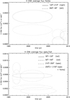 |
Fig. 2. Energy-averaged hydrogen ENA flux measurements by HSTOF. The upper panel shows the ENA flux from the flank directions (120° − 210° and 300° − 30° ecliptic longitude sectors). The lower panel shows the flux from the forward sector (210° − 300°), the forward + flanks sector (255° ± 155°), and the heliotail sector (30° − 120° or 50° − 100°). The data are shown as ellipses; the vertical semiaxes represent statistical 1σ deviations and the horizontal axes indicate time intervals. |
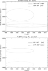 |
Fig. 3. As Fig. 2 but for the case of helium ENA. The upper panel shows He ENA flux from the flank directions (120° − 210° and 300° − 30° ecliptic longitude sectors). The lower panel shows the flux from the forward sector (210° − 300°) and heliotail sector (30° − 120°). |
3. Comparing the observation regions of HSTOF and Voyager 1
The flux JENA of the ENA originating in the heliosheath can be approximately expressed as (1)
(1)
where Jion is the parent ion flux (protons for hydrogen ENA, He+ for helium ENA) at the same energy as JENA, σcx, H, and σcx, He are the cross sections for charge exchange between the parent ions and the neutral hydrogen or neutral helium background gas of density nH and nHe, respectively, and L is the thickness of the source region along the line of sight (LOS). The values Jion and nH are averages over the distance along the LOS within the source region (the inner heliosheath). For the helium ENA, we omitted the additional contribution from double charge exchange between the He++ and the neutral He background, which is on the order of 3% (Swaczyna et al. 2017). The equation does not include the ENA losses on the way from the source, but in the energy range where most of the ENA observations are carried out (IBEX Hi, INCA, and HSTOF) these effects are relatively small (about 1% for HSTOF).
To compare the observations of Voyager 1 and HSTOF we use the ENA flux averaged over the HSTOF energy range: E1 < E < E2 where E1 = 58 keV and E2 = 88 keV. Eq. (1) then becomes (2)
(2)
where ⟨A⟩ denotes the average over the HSTOF energy range (3)
(3)
When used for the case of HSTOF, Eq. (2) must also be averaged over directions of the lines of sight, and over the observation time periods. As explained in Sect. 2, we divide the HSTOF field of view into four ecliptic longitude sectors (Fig. 1). Because of proximity to the Voyager 1 and 2 trajectories, the forward (LISM apex) sector is most suitable for comparison with Voyager observations. A study of the energetic ion distribution in the heliosheath (Czechowski et al. 2012) and the Bonn model of the heliosphere, on which this study was based (Fahr et al. 2000), implies that the thickness L, the energetic ion fluxes, and the neutral density do not vary much over this region. We also consider the two flank sectors. Table 1 lists the hydrogen ENA flux values, which is also illustrated in the Fig. 2.
Table 1 includes also the estimated hydrogen ENA flux  from the Voyager 1 direction. It is calculated by substituting for Jion in Eq. (2) the energetic proton flux Jp, V1 at Voyager 1 and for L the distance LV1 = 28 AU between the termination shock and the cliff along the Voyager 1 trajectory. In the HSTOF energy range, Voyager 1 LECP measures only the Z ≥ 1 ion flux
  , which includes the protons along with the heavier ions. We assume that Jp, V1 is approximately equal to
  . For JZ ≥ 1, V1 we use the same power-law fit as in Hsieh et al. (2010), i.e.,
  , where A = 183.5, γ = 1.6, E is in keV and J in (cm2 s sr keV)−1. For σcx, H(E) we use the formula of Lindsay & Stebbings (2005). For σcx, He(E) the interpolation formula from the Redbook (Barnett et al. 1990) is used.
We approximate the neutral densities nH and nHe in the observation regions of Voyager 1 and HSTOF (the forward sector) using the values determined from observations as follows: nH = 0.089 ± 0.022 cm−3 (Bzowski et al. 2008; Bzowski et al. 2009; Richardson et al. 2008) and nHe = 0.015 ± 0.003 cm−3 (Witte 2004; Gloeckler et al. 2004). A detailed discussion of the methods involved is given in Appendices A (nH) and B (nHe). As pointed out in the appendices, estimations by various methods lead to similar values of the neutral densities. In the case of hydrogen, the estimated nH is the value at the termination shock. We use this value in place of the average across the inner heliosheath, which is probably (according to numerical models; see Müller et al. 2008) higher by 15−20% due to ionization losses. For neutral helium the ionization losses are lower than for hydrogen, such that the value of nHe derived from observations is expected to be a good approximation of the average along the LOS across the inner heliosheath. The errors in ⟨JENH, V1⟩ include only the errors in nH and nHe.
The third column of Table 1 shows the effective thickness Leff, defined by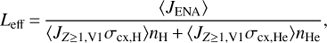 (4)
(4)
where ⟨JENA⟩ is the hydrogen ENA flux measured by HSTOF in a given sector, and  , nH and nHe are defined in the previous paragraphs. The value Leff is the thickness (of the ENA source region) needed to reproduce the measured HSTOF flux under assumption that the parent proton flux in the source region is the same as the average of Voyager 1 Z ≥ 1 ion flux along its trajectory.
In all cases except the time period 1996−1997, the values of Leff are significantly lower (by more than 1σ) than the value of 28 AU measured by Voyager 1. For the case of apex, 1996−2005 time period, Leff is lower than the value of 21 ± 6 AU obtained by Hsieh et al. (2010) using the same HSTOF data, but neglecting the contribution from charge exchange with neutral He.
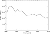 |
Fig. 4. Solar wind flux (yearly averages based on OMNI2 data) at 1 AU as a function of time. The time interval starts earlier than the HSTOF observations discussed in this paper because of expected delay between the changes in the solar wind and in the ion distributions in the heliosheath. |
Hydrogen ENA flux from HSTOF and estimation for Voyager 1 direction.
4. Discussion
In this section we discuss some important topics related to the observations by HSTOF: (1) high ENA flux from the heliotail direction, (2) asymmetry of the flux from the flank sectors, and (3) timescales of temporal evolution of the ENA flux.
4.1. ENA flux from the heliotail
At present, HSTOF is the only ENA instrument that has observed the maximum of the ENA flux coming from the heliotail (ISM anti-apex) direction. This can be interpreted as a signature of the extended heliotail (see, e.g., Czechowski et al. 2006). An alternative explanation proposed by Kota et al. (2001) predicted a value of the ENA flux that is too low.
The uniqueness of HSTOF can be explained by the fact that the energy range of the ENA observation by HSTOF (58−88 keV for hydrogen) is higher than the energy range of other instruments, i.e., IBEX (0.7−4.3 keV) and INCA (5.2−55 keV).
In Appendix C we present a toy model of the energetic ion distribution between the termination shock and heliopause, assuming that the heliosphere has an extended tail (is comet-like), and that convection by plasma and neutralization by charge exchange are, respectively, the main transport and loss mechanisms. We show that, above some crossover energy, the ENA flux from the heliotail direction exceeds the flux from the apex direction. With reasonable assumptions about the model parameters, the crossover occurs at ∼46 keV.
This conclusion agrees with a more detailed model calculation (Czechowski et al. 2012) based on the Bonn model of the heliosphere (Fahr et al. 2000), and including approximate description of adiabatic acceleration, parallel diffusion, charge-exchange neutralization, and the loss due to escape across the heliopause. In this case the ENA flux from the heliotail exceeds the flux from the forward direction for energies above ∼40 keV. This value, as well as the toy model result, are close to the upper limit of INCA (55 keV).
For INCA, the peak ENA fluxes from the nose and anti-nose sectors are similar (Dialynas et al. 2013; Dialynas et al. 2017). Figure 3a of Dialynas et al. (2017) for energies 5.2−13.5 keV and 35−55 keV suggests the anti-nose/nose peak ratio of ∼0.5−1. For IBEX-Hi (0.7−4.4 keV) the ratio estimated from Schwadron et al. (2014) is between 0.76 and 0.95 (average 0.83). The IBEX data are averaged over the first five years of operation (2009−2013), the ecliptic latitude range −21° to 21°, and the ecliptic longitudes corresponding to the right (120° − 210°) and left (300° − 30°) flank sectors of HSTOF. In Fig. 6 we compare these estimations with the predictions of the toy model.
Figure 7 shows our estimation of time-dependence of the tail/apex ENA flux ratio based on the observations by IBEX and INCA. In the case of IBEX, we use two sources. From Schwadron et al. (2014), we take the ENA flux from the nose and tail directions, averaged over the period 2009−2013. This we combine with the time-dependent flux data for the same time period (with the flux normalized to 1 at the year 2009), provided by Fig. 8 of Zirnstein et al. (2017).
In the case of INCA, we use the data from Fig. 2 of Dialynas et al. (2017), covering the time period from 2004.5 to 2013.5. We use the flux from the tail measured at ecliptic latitudes between −20° and 0°. Since the time-dependent ENA flux data from the nose direction are not provided, we follow Dialynas et al. (2017) and use instead the ENA flux from the direction of Voyager 1 or, after the year 2010, from the direction of Voyager 2. We note that both Voyagers are in the forward part of the heliosheath (see Fig. 5). The ENA flux from the Voyager directions may therefore be used as a rough approximation of the flux from the nose direction. Time dependence of the ENA flux as observed by IBEX and INCA is briefly reviewed in Appendix D.
 |
Fig. 5. Schematic view of the heliosphere from the interstellar inflow direction, and, in the upper right part of the figure, the view in the (v, B) plane. The shape of the heliosphere is affected by the interstellar magnetic field. The heliosphere is compressed in the direction perpendicular to the (v, B) plane, but also becomes asymmetric in the (v, B) plane. This effect can lead to the asymmetry between the right and left flanks of the heliosphere, as observed by HSTOF. |
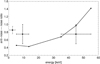 |
Fig. 6. Tail/apex ENA flux ratio. Crosses show our estimations using the data of IBEX Hi (0.7−4.4 keV, Schwadron et al. 2014) averaged over the period 2009−2013, and INCA (5.2−13.5 and 35−55 keV, Dialynas et al. 2017, Fig. 3a, average over the period 2003−2009). The continuous line indicates the toy model prediction. |
4.2. Radial widths of the HSTOF flank sectors
The HSTOF data (Figs. 2 and 3) show that the ENA flux from the right flank region (ecliptic longitude 120° − 210°) is higher than from the left flank (300° − 30°). An interesting possibility is that this observation is related to the asymmetry of the heliosphere induced by the interstellar magnetic field B. The asymmetry can be estimated using models of the heliosphere based on numerical MHD solutions.
We use the state-of-art model by Heerikhuisen et al. (Heerikhuisen & Pogorelov 2010) with a kinetic treatment of the neutral hydrogen component. The solar wind and interstellar parameters used in this model (number 4 in Table 2) are identical to those obtained by Zirnstein et al. (2016) from analysis of IBEX ENA observations, constrained by the Voyager crossings of the termination shock and heliopause. In particular, the model conforms with measurements of the ISM velocity V, and the probable direction of the interstellar magnetic field B (near the IBEX ribbon center).
Figure 8 shows the structure of the heliosphere in the ecliptic plane based on this model. The termination shock and heliopause are shown by solid lines. The right and left flank regions are shaded. The ratio of the right flank mean width to the left flank mean width (⟨r/l⟩) is 1.4 (Table 2).
For comparison, we also present results from three simpler models (1–3 in Table 2) using the Warsaw MHD code (Ratkiewicz & Grygorczuk 2008), which assumes a constant neutral background. All these models share the same (B, V) plane, which is the symmetry plane of the outer heliosheath. The parameters of the ISM (the magnetic field strength B, plasma density np, angle α(B, V) between B and V, and the temperature T), and the values of ⟨r/l⟩, are given in Table 2.
The HSTOF ENA energy-averaged flux ratio from the flanks for the period 1996−2005 (Figs. 2 and 3) is 2.0 ± 0.9 for H and 2.2 ± 1.2 for He, which is higher than the ⟨r/l⟩ values given in Table 2, although within statistical errors.
For lower ENA energy, we estimate the right flank/left flank ENA flux ratio from digitalized IBEX-Hi ENA maps for the globally distributed flux (without the ribbon contribution, Schwadron et al. 2014). The results are between 1.14 and 1.45 (average 1.27) for IBEX Hi energy channels (0.7−4.3 keV). For the case of INCA, a similar estimation is difficult because there is a gap in the data coverage inside the left flank region (Dialynas et al. 2017, Fig. 3a).
Since the spatial distribution of the ENA parent ions in the inner heliosheath is in general nonuniform, the geometrical ⟨r/l⟩ ratio may be different from the ENA flux ratio. In particular, according to the HSTOF data, the right flank/left flank ENA flux ratio becomes close to 1 during the low flux period after the year 2005 (Figs. 2 and 3). A detailed study of the relation between the geometry of the heliosphere and the ENA flux distribution is beyond the scope of this work.
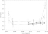 |
Fig. 7. Estimations of the tail/apex ENA flux ratio as the function of time, based on the results from IBEX (solid lines) and INCA (dashed lines). The following cases are shown: (1) INCA, ENA energy 35−55 keV; (2) INCA, ENA energy 5−13 keV; (3) IBEX, ENA energy 4.3 keV; and (4) IBEX, ENA energy 0.7 keV. In the case of INCA, the ENA flux from the nose direction is replaced by the flux from Voyager 1 or Voyager 2 directions. See the text for detailed description. |
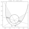 |
Fig. 8. View of the heliosphere in the ecliptic plane (model 4 in Table 2). The boundaries of the flank regions are shown. The right flank is 1.4 times thicker than the left flank; we use mean thickness in the radial direction. The axes are scaled in AU. The ISM inflow direction is approximately along the vertical axis. |
Flank sector widths in the MHD models.
4.3. Convection time and limits on time dependence of the heliospheric ENA flux
The ENA fluxes measured by HSTOF show a significant decrease over the first ten years of operation (1996−2006) that continues in the subsequent period. An important question is whether this decrease is consistent with characteristic timescales of ENA propagation and production in the inner heliosheath.
We assume that the parent ions of the HSTOF ENA are accelerated at the termination shock and transported into the inner heliosheath by plasma convection. During the process, some of these parent ions are lost by conversion into ENA. In the HSTOF energy range, the ENA velocities (above 2300 km s−1 for He and 3300 km s−1 for H atoms) are much higher than the inner heliosheath plasma speed (below ∼100 km s−1). The propagation time of the ENA to the observer is therefore much shorter than the convection time of the parent ion from the termination shock to the LOS of the observer.
We define a characteristic time τ for the ENA flux as the average over the length of the LOS of the convection time τc, weighted by the local value of the energetic ion flux Jion(E) (the parent ions of the ENA), i.e., (5)
(5)
where r is the point on the LOS at which the flow line ends. The integration runs over the part of the LOS between the termination shock and heliopause. The interpretation of τ as a characteristic time for variation of the ENA flux is supported by our analytical toy model (see Appendix C).
To calculate τ we use selected models of the heliosphere from Table 2. The method of calculation of the ion flux is described in Appendix E. The results are collected in Table 3.
The increase of τ with the ENA energy seen in Table 3 reflects the smaller loss factors (smaller σcx) for higher energy ions. The fraction of high energy ions reaching the more distant parts of the LOS is therefore larger than the fraction of lower energy ions. Consequently, the weighted average of τc over the LOS is larger for high energy than for low energy ENA.
ENA decay times.
4.4. Time dependence of HSTOF ENA flux
Let us now consider the HSTOF ENA data (Figs. 2 and 3) in view of the results obtained in the preceding subsection.
The decreases in the solar wind flux were observed at 1 AU during the periods 1992.5−1994.5, 1997.5−1999.5, and 2005.5−2008.5 (Fig. 4). Solar wind propagation to the termination shock takes ∼1 yr. The energy- and model-averaged values of τ from Table 3 are 3, 10, 6, and 4.5 yr for the forward, tail, right flank, and left flank sectors, respectively. We would, therefore, expect the larger part of the change in the ENA flux to take a time on the order τ after the arrival of the solar wind perturbation at the shock. The observed changes in the HSTOF hydrogen ENA flux are:
-
(1)
in the forward sector, a drop by 71% between 1996−1997 and 1998−2005, dt = 5 yr;
-
(2)
in the extended forward sector, a drop by 32% between 1996−1997 and 1998−2003, dt = 4 yr;
-
(3)
in the tail sector, a drop by 25% between 1996−1997 and 1998−2003, dt = 4 yr;
-
(4)
in the right flank, a drop by 78% between 1996−2005 and 2006−2010, dt = 7.5 yr (we have combined the two low flux 2006−2008 and 2008−2010 periods),
For the forward and right flank sectors, where the observed change in the flux is large, dt > τ. For extended forward sector, we can take τ as the average of values for the forward and both flank sectors, which gives τ = 4.5 yr; this value is comparable to dt.
For the tail sector, dt is significantly smaller than τ, but the change in the ENA flux is small, which may suggest that only a part of the total change in the heliotail ENA flux has been observed.
The events (1), (2), and (3) could be attributed to the 1992.5−1994.5 solar wind decrease. Event (4) can also be related to the 1997.5−1999.5 decrease. Altogether, we conclude that the time evolution of the ENA flux observed by HSTOF is consistent with the timescales derived in the previous subsection.
5. Conclusions
The ENA data from HSTOF obtained over the period 1996−2010 show a significant decrease in the flux intensity. Although the time dependence cannot be resolved in detail, the hydrogen ENA data for the apex and tail sectors (Fig. 2, lower panel) suggest a large drop in solar wind flux occurring soon after the first two years (1996−1997) of operation of HSTOF. The decreases of the ENA flux observed by IBEX (McComas et al. 2017) and INCA (Dialynas et al. 2017) refer to a later time period (after 2010). The recent IBEX data show the ENA flux increasing in response to the solar wind intensification (McComas et al. 2018).
The low values of the ENA flux resulting from the decrease are in tension with observations by Voyagers of the energetic ions in the inner heliosheath. If the energetic proton intensity in the HSTOF ENA source region were as high as measured by Voyagers, the HSTOF data obtained after the year 1997 would indicate an unexpectedly small thickness of the inner heliosheath in the field of view of HSTOF (±17° from the ecliptic plane).
The difference in the ENA fluxes measured by HSTOF and the value estimated from Voyager LECP energetic ion data may be attributed to the differences between the regions in space observed by these two instruments. The differences could involve (1) the geometrical thickness L, (2) the energetic ion flux density ⟨Jp⟩, or (3) the background neutral gas density nH and nHe.
If the ENA flux decrease occurs on a short timescale, the most likely possibility is probably (2). A change by a large factor in the size of the inner heliosheath, or in the density distribution of neutral atoms coming in from the interstellar medium, requires a longer time. Moreover, if the parent ions of the ENA measured by HSTOF derive from acceleration of the pick-up ions of the solar wind, the energetic ion flux distribution would reflect the heliolatitude-dependent solar wind structure. A decrease in the energetic ion density restricted to the HSTOF field of view (near the solar equator plane) is then a natural possibility. The ENA flux decrease may then be related to the decrease in the solar wind flux (Fig. 4).
The IBEX map of the distributed ENA flux (ribbon-subtracted, attributed to the heliospheric rather than outer sources; Schwadron et al. 2011, Fig. 8) show, in fact, a valley of relatively low ENA flux near the ecliptic for the highest energy IBEX channels, with Voyagers positions near the valley rims. A similar structure can be seen in the INCA maps (Dialynas et al. 2013). This feature can be understood as due to predominance of the slow solar wind near the ecliptic, and consequently a lower energy of the pick-up ions produced in this region. The energetic ion flux in the HSTOF observation region may, therefore, be substantially lower than the value obtained by simple interpolation between the Voyager 1 and Voyager 2 data. A low flux of energetic ions could explain the HSTOF ENA observations without the need of assuming very low values of geometrical thickness L.
An alternative possibility would be the existence of an indentation in the shape of the heliopause (or the heliocliff) along the ecliptic plane. Such a structure may be related to the effective weakening of the solar magnetic field in the sectored region and was indeed predicted by one early numerical model (Washimi & Tanaka 2001). This result was, however, not confirmed by later calculations. Moreover, if the low value of the high energy ENA flux near the ecliptic would follow solely from the reasons of geometry, one would expect the same feature to persist for low energy ENA. The difference between the IBEX maps for the highest and lowest energy IBEX ENA channels disfavors this possibility.
The important question is whether the HSTOF results can be affected by a systematic error leading to the underestimation of the ENA flux from HSTOF. The repeat of the in-flight cross calibration with ACE confirmed that the agreement between the HSTOF and ACE high energy ion channels continues to hold. In particular, although the HSTOF ENA flux was decreasing, there was no decrease observed in the ratio of the high energy HSTOF to the ACE ion flux data. One conclusion is that the efficiency of the HSTOF detector did not change during the period between the cross calibrations, such that the observed flux decrease cannot be attributed to the deterioration of the detector.
The discussion in Sects. 4.3 and 4.4 implies that the time evolution observed in the HSTOF ENA data is consistent with the timescales derived for the heliosphere with an extended tail (the comet-like heliosphere). The observations with better time resolution may, however, affect this conclusion. A sharp drop in the ENA flux from the heliotail direction has been observed by INCA (Dialynas et al. 2017).
Finally, we note that the excess of the ENA flux from the right flank over the flux from the left flank, observed by HSTOF in the period 1996−2005, may be related to the asymmetry of the heliosphere caused by the interstellar magnetic field pointing close to the center of the IBEX ribbon.
Acknowledgments
We thank Jacob Heerikhuisen for permission to use the results of his MHD simulation. A part of this research was supported by Polish NCN grant 2015/19/b/ST9/01328. A.C. appreciates the hospitality provided by the Max Planck Institut fur Sonnensystemforschung, where part of this work was carried out.
References
- Banaszkiewicz, M., Witte, M., & Rosenbauer, H. 1996, A&AS, 120, 587 [NASA ADS] [CrossRef] [EDP Sciences] [Google Scholar]
- Baranov, V., & Malama, Y. 1993, J. Geophys. Res., 98, 15157 [NASA ADS] [CrossRef] [Google Scholar]
- Barnett, C. F., Hunter, H. T., Kirkpatrick, M. I., Alvarez, I., & Phaneuf, R. A. 1990, in Atomic Data for Fusion. Collisions of H, H2, He and Li Atoms and Ions with Atoms and Molecules (Oak Ridge, TN: Oak Ridge Natl. Lab.), Report ORNL-6086-VI [Google Scholar]
- Bochsler, P., Kucharek, H., Möbius, E., et al. 2014, ApJS, 210, 12 [NASA ADS] [CrossRef] [Google Scholar]
- Bzowski, M., Möbius, E., Tarnopolski, S., Izmodenov, V., & Gloeckler, G. 2008, A&A, 491, 7 [NASA ADS] [CrossRef] [EDP Sciences] [Google Scholar]
- Bzowski, M., Möbius, E., Tarnopolski, S., Izmodenov, V., & Gloeckler, G. 2009, Space Sci. Rev., 143, 177 [NASA ADS] [CrossRef] [Google Scholar]
- Bzowski, M., Sokół, J. M., Tokumaru, M., et al. 2013a, ISSI Scientific Report, 13, 67 [Google Scholar]
- Bzowski, M., Sokół, J. M., Kubiak, M. A., & Kucharek, H. 2013b, A&A, 557, A50 [NASA ADS] [CrossRef] [EDP Sciences] [Google Scholar]
- Cummings, A. C., Stone, E. C., & Steenberg, C. D. 2002, ApJ, 578, 194 [NASA ADS] [CrossRef] [Google Scholar]
- Czechowski, A., Hilchenbach, M., & Kallenbach, R. 2006, in The Physics of the Heliospheric Boundaries, eds. V. Izmodenov, & R. Kallenbach (ESA Publications Division, EXTEC) [Google Scholar]
- Czechowski, A., Hilchenbach, M., Hsieh, K. C., Grzedzielski, S., & Kóta, J. 2008, A&A, 487, 329 [NASA ADS] [CrossRef] [EDP Sciences] [Google Scholar]
- Czechowski, A., Hilchenbach, M., & Hsieh, K. C. 2012, A&A, 541, A14 [NASA ADS] [CrossRef] [EDP Sciences] [Google Scholar]
- Decker, R. B., Krimigis, S. M., Roelof, E. C., et al. 2005, Science, 309, 2020 [NASA ADS] [CrossRef] [PubMed] [Google Scholar]
- Dialynas, K., Krimigis, S. M., Mitchell, D. G., Roelof, E. C., & Decker, R. B. 2013, ApJ, 778, 13 [CrossRef] [Google Scholar]
- Dialynas, K., Krimigis, S. M., Mitchell, D. G., Decker, R. B., & Roelof, E. C. 2017a, Nat. Astron., 1, 0115 [CrossRef] [Google Scholar]
- Dialynas, K., Krimigis, S. M., Mitchell, D. G., Decker, R. B., & Roelof, E. C. 2017b, J. Phys. Conf. Ser., 900, 012005 [CrossRef] [Google Scholar]
- Fahr, H. J., & Ruciński, D. 2001, Space Sci. Rev., 97, 407 [NASA ADS] [CrossRef] [Google Scholar]
- Fahr, H. J., Kausch, T., & Scherer, K. 2000, A&A, 357, 268 [NASA ADS] [Google Scholar]
- Florinski, V., Zank, G. P., & Pogorelov, N. V. 2005, J. Geophys. Res., 110, A07104 [NASA ADS] [CrossRef] [Google Scholar]
- Gloeckler, G., & Geiss, J. 2001, AIP Conf. Proc., 598, 281 [NASA ADS] [CrossRef] [Google Scholar]
- Gloeckler, G., Möbius, E., Geiss, J., et al. 2004, A&A, 426, 845 [NASA ADS] [CrossRef] [EDP Sciences] [Google Scholar]
- Heerikhuisen, J., & Pogorelov, N. V. 2010, ASP Conf. Ser., 429, 227 [NASA ADS] [Google Scholar]
- Heerikhuisen, J., Florinski, V., & Zank, G. P. 2006, J. Geophys. Res., 111, A06110 [NASA ADS] [CrossRef] [Google Scholar]
- Hilchenbach, M., Hsieh, K. C., Hovestadt, D., et al. 1998, ApJ, 503, 916 [NASA ADS] [CrossRef] [Google Scholar]
- Hilchenbach, M., Hsieh, K. C., Hovestadt, D., et al. 2001, COSPAR Colloq. Ser., 11, 273 [CrossRef] [Google Scholar]
- Hilchenbach, M., Czechowski, A., Hsieh, K. C., & Kallenbach, R. 2006, AIP Conf. Proc., 858, 276 [NASA ADS] [CrossRef] [Google Scholar]
- Hilchenbach, M., Kallenbach, R., Hsieh, K. C., & Czechowski, A. 2012, AIP Conf. Proc., 1436, 227 [NASA ADS] [CrossRef] [Google Scholar]
- Hovestadt, D., Hilchenbach, M., Bürgi, A., et al. 1995, Sol. Phys., 162, 441 [NASA ADS] [CrossRef] [Google Scholar]
- Hsieh, K. C., Giacalone, J., Czechowski, A., et al. 2010, ApJ, 718, L185 [NASA ADS] [CrossRef] [Google Scholar]
- Izmodenov, V., Gloeckler, G., & Malama, Y. 2003a, Geophys. Res. Lett., 30, 1351 [NASA ADS] [CrossRef] [Google Scholar]
- Izmodenov, V., Malama, Yu G., Gloeckler, G., & Geiss, J. 2003b, ApJ, 594, L59 [NASA ADS] [CrossRef] [Google Scholar]
- Kota, J., Hsieh, K. C., Czechowski, A., Jokipii, J. R., & Hilchenbach, M. 2001, J. Geophys. Res., 106, 24907 [NASA ADS] [CrossRef] [Google Scholar]
- Krimigis, S. M., Decker, R. B., Roelof, E. C., et al. 2013, Science, 341, 144 [NASA ADS] [CrossRef] [PubMed] [Google Scholar]
- Lindsay, B. G., & Stebbings, R. F. 2005, J. Geophys. Res., 110, A12213 [NASA ADS] [CrossRef] [Google Scholar]
- McComas, D. J., Angold, N., Elliott, H. A., et al. 2013, ApJ, 779, 2 [Google Scholar]
- McComas, D., Zirnstein, E. J., Bzowski, M., et al. 2017, ApJS, 229, 41 [NASA ADS] [CrossRef] [Google Scholar]
- McComas, D. J., Dayeh, M. A., Funsten, H. O., et al. 2018, ApJ, 856, 6 [CrossRef] [Google Scholar]
- McMullin, D. R., Bzowski, M., Moebius, E., et al. 2004, A&A, 426, 885 [NASA ADS] [CrossRef] [EDP Sciences] [Google Scholar]
- Moebius, E., Bochsler, P., Bzowski, M., et al. 2012, ApJS, 198, 11 [NASA ADS] [CrossRef] [Google Scholar]
- Müller, H.-R., Frisch, P. C., Florinski, V., & Zank, G. P. 2006, ApJ, 647, 1491 [NASA ADS] [CrossRef] [Google Scholar]
- Müller, H.-R., Florinski, V., Heerikhuisen, J., et al. 2008, A&A, 491, 43 [NASA ADS] [CrossRef] [EDP Sciences] [Google Scholar]
- Müller, H. R., Bzowski, M., Moebius, E., & Zank, G. P. 2013, AIP Conf. Proc., 1539, 348 [NASA ADS] [CrossRef] [Google Scholar]
- Pryor, W., Gangopadhyay, P., Sandel, B., et al. 2008, A&A, 491, 21 [NASA ADS] [CrossRef] [EDP Sciences] [Google Scholar]
- Ratkiewicz, R., & Grygorczuk, J. 2008, Geophys. Res. Lett., 35, L23105 [NASA ADS] [CrossRef] [Google Scholar]
- Richardson, J. D., Liu, Y., Wang, C., & McComas, D. J. 2008, A&A, 491, 1 [NASA ADS] [CrossRef] [EDP Sciences] [Google Scholar]
- Rucinski, D., & Fahr, H. J. 1989, A&A, 224, 290 [NASA ADS] [Google Scholar]
- Rucinski, D., Bzowski, M., & Fahr, H. J. 1998, A&A, 334, 337 [NASA ADS] [Google Scholar]
- Scherer, K., & Fahr, H.-J. 2003a, Geophys. Res. Lett., 30, 17 [NASA ADS] [CrossRef] [Google Scholar]
- Scherer, K., & Fahr, H.-J. 2003b, A&A, 404, L47 [NASA ADS] [CrossRef] [EDP Sciences] [Google Scholar]
- Schwadron, N. A., Allegrini, F., Bzowski, M., et al. 2011, ApJ, 731, 56 [NASA ADS] [CrossRef] [Google Scholar]
- Schwadron, N. A., Moebius, E., Fuselier, S. A., et al. 2014, ApJS, 215, 13 [NASA ADS] [CrossRef] [Google Scholar]
- Sokół, J. M., Bzowski, M., Tokumaru, M., Fujiki, K., & McComas, D. J. 2013, Sol. Phys., 285, 167 [Google Scholar]
- Stone, E. C., Cummings, A. C., McDonald, F. B., et al. 2005, Science, 309, 2017 [NASA ADS] [CrossRef] [PubMed] [Google Scholar]
- Stone, E. C., Cummings, A. C., McDonald, F. B., et al. 2013, Science, 341, 150 [NASA ADS] [CrossRef] [PubMed] [Google Scholar]
- Swaczyna, P., Grzedzielski, S., & Bzowski, M. 2017, ApJ, 840, 75 [NASA ADS] [CrossRef] [Google Scholar]
- Tarnopolski, S., & Bzowski, M. 2009, A&A, 493, 207 [NASA ADS] [CrossRef] [EDP Sciences] [Google Scholar]
- Thomas, G. E. 1978, Ann. Rev. Earth Plant Sci., 6, 173 [NASA ADS] [CrossRef] [Google Scholar]
- Wang, C., Richardson, J. D., & Gosling, J. T. 2000, Geophys. Res. Lett., 27, 2429 [NASA ADS] [CrossRef] [Google Scholar]
- Washimi, H., & Tanaka, T. 2001, Adv. Space Res., 27, 509 [NASA ADS] [CrossRef] [Google Scholar]
- Webber, W. R., & McDonald, F. B. 2013, Geophys. Res. Lett., 40, 1665 [NASA ADS] [CrossRef] [Google Scholar]
- Witte, M. 2004, A&A, 426, 835 [NASA ADS] [CrossRef] [EDP Sciences] [Google Scholar]
- Witte, M., Banaszkiewicz, M., & Rosenbauer, H. 1996, Space Sci. Rev., 78, 289 [NASA ADS] [CrossRef] [Google Scholar]
- Wood, B. E., Müller, H.-R., & Witte, M. 2015, ApJ, 801, 62 [NASA ADS] [CrossRef] [Google Scholar]
- Zirnstein, E. J., Funsten, H. O., Heerikhuisen, J., et al. 2016, ApJ, 826, 58 [NASA ADS] [CrossRef] [Google Scholar]
- Zirnstein, E. J., Heerikhuisen, J., Zank, G. P., et al. 2017, ApJ, 836, 238 [NASA ADS] [CrossRef] [Google Scholar]
Appendix A:
Determination of hydrogen density nH
In this section we present two methods used to obtain an estimation of the neutral hydrogen density in the heliosheath and the corresponding results.
Bzowski et al. (2008) estimated the density of interstellar hydrogen in the nose region of the termination shock using the results of the hydrogen pickup ion flux measurements on Ulysses from SWICS (Gloeckler & Geiss 2001). These authors developed an approach that minimizes the error in the derived density due to the uncertainty in the ionization rate βion of hydrogen in the heliosphere. The production rate of the pick-up ions at the distance r from the Sun is given by the product of the ionization rate and local hydrogen density nH(r): S(r) = βion(r)nH(r). Since nH(r) decreases as the value of βion goes up, the derivative dS/dβ must be equal to zero at some distance from the Sun. For the heliospheric conditions during the Ulysses observations used by Bzowski et al. (2008) Ulysses was located close to this special distance. The approach, which can be proven strictly in the framework of the cold gas approximation, was verified using a detailed model of the neutral hydrogen distribution (Tarnopolski & Bzowski 2009) based on realistic, measurement-based ionization rates and radiation pressure. The neutral hydrogen density at the termination shock was obtained by matching these simulations with the results of global models of the heliosphere based on kinetic Monte Carlo treatment of the neutral hydrogen component (Baranov & Malama 1993; Izmodenov et al. 2003; Izmodenov et al. 2003). The result was nH = 0.087 ± 0.003 cm−3, where the uncertainty is due to uncertainties in the modeling, ionization rates, and radiation pressure. When the measurement uncertainty of the pick-up ion production rate is added (mostly due to the uncertainty in the geometric factor of the instrument: Gloeckler & Geiss 2001), the total uncertainty increases to about 25%.
Richardson et al. (2008) estimated the density of interstellar hydrogen at the termination shock using a totally independent method. They started from the prediction by Fahr & Ruciński (2001) that because of mass loading of the solar wind by pickup ions, the momentum flow of the solar wind inside the termination shock is reduced, and the amount of the resulting slowdown can be utilized to determine the density of neutral interstellar hydrogen at the termination shock.
Pickup ions in the solar wind are produced predominantly by three ionization reactions: charge exchange with solar wind protons, photoionization, and ionization by solar wind electron impact (for recent review, see Bzowski et al. 2013). Taken collectively over a long stretch between the Sun and termination shock, these contributions produce a net effect of the solar wind slowdown in the nose region by ∼15%.
Richardson et al. (2008) compared the solar wind expansion speed at Ulysses and at Voyager 2 when they were close to radial alignment; the first spacecraft
was at ∼5 AU from the Sun while the other was approaching the termination shock at ∼80 AU. They discovered that the difference in the solar wind expansion speed is approximately 60 km s−1. They paid attention to a possible slowdown for reasons not related to the interaction of the solar wind with neutral interstellar gas. Using a 1D MHD model of the solar wind with pickup ions (Wang et al. 2000), they fitted predicted slowdown of the solar wind expansion speed for the conditions of the Ulysses and Voyager observations and found a match for the solar wind density at the termination shock equal to 0.09 cm−3 that has a fit error of 0.01 cm−3. Given the approximate character of the background hydrogen density model they used – it was a cold model with an ionization rate slightly different from the actually measured solar wind and ionization parameters used by Bzowski et al. (2008) – and the relatively large uncertainty of the result of Bzowski et al. (2008), the agreement between these two results is excellent.
Another, albeit qualitative, test for the robustness of the determination of the density of neutral hydrogen at the termination shock was carried out by Pryor et al. (2008), who used combined observations of the heliospheric Lyman-α glow from Voyager 1 and Cassini, and a sophisticated model of solar Lyman-α radiation transport in the heliosphere to verify that the density values from Bzowski et al. (2008) and Richardson et al. (2008) are not at odds with the extreme-ultraviolet measurements.
Finally, Bzowski et al. (2009) proposed the density at the termination shock equal to 0.089 ± 0.022 cm−3, calculated as a weighted average of the results from Bzowski et al. (2008) and Richardson et al. (2008). The neutral hydrogen density in the LIC in front of the heliosphere was proposed to be equal to 0.16 ± 0.04 cm−3. This result, especially for the density at the termination shock, seems very robust since it was demonstrated to depend very little on the assumptions and uncertainties in the modeling.
As it results from all modern models of the heliosphere (Baranov & Malama 1993; Heerikhuisen et al. 2006; Florinski et al. 2005; Müller et al. 2006; Scherer & Fahr 2003; Scherer & Fahr 2003), recapitulated by Müller et al. (2008), the expected departures of neutral interstellar hydrogen density in the upwind hemisphere from the value at the termination shock are about 15−20%, which is on the order of the uncertainty reported by Bzowski et al. (2008).
Appendix B:
Determination of neutral helium density
The density of neutral interstellar helium at the termination shock was determined using the direct sampling method on GAS/Ulysses witte04 and via interpretation of He+ and He++ pickup ion measurements on SWICS/Ulysses and SWICS/ACE (Gloeckler et al. 2004). The results of the three measurements were in a very good agreement with each other.
Interstellar helium penetrates the heliosheath with very little attenuation in the heliospheric interface region (less than 10%, Müller et al. 2013). The main loss mechanisms inside the termination shock are photoionization (see, e.g., Bochsler et al. 2014) and electron impact ionization (Rucinski & Fahr 1989). The radial profile of the electron impact ionization rate is far from trivial (see McMullin et al. 2004; Bzowski et al. 2013; Bzowski et al. 2013). The loss due to charge exchange with solar wind ions is negligible. A recent review of the helium loss processes was provided by Bzowski et al. (2013).
The direct sampling method employed in the analysis of GAS measurements, extensively presented by Banaszkiewicz et al. (1996), consists in measuring the distribution on sky of the flux of neutral interstellar He as seen from a spacecraft moving around the Sun, and fitting the parameters of the distribution function of the helium gas in the source region (the LIC). The density determination involves three important assumptions: (1) the form of the distribution function of neutral helium outside the heliosphere (commonly assumed to be given by the Maxwell-Boltzmann distribution), (2) the radial and latitudinal profiles of the ionization rate, and (3) the absolute sensitivity of the detector.
At the time of GAS/Ulysses measurements, the knowledge of helium ionization rates was limited because of the lack of suitable observations (McMullin et al. 2004). The lack of exact knowledge of the absolute level of the ionization rate can be alleviated if it is possible to measure the direct and indirect beams of neutral helium simultaneously.
Successful detection of the indirect beam was achieved by Witte et al. (1996) in only a few observations and the ratio measured was so low that it became affected by the background level. The determination of interstellar He density had, therefore, to rely on the direct beam; the ionization was taken either from McMullin et al. (2004) or from the authors’ own fits. Thus the range of derived densities was relatively broad, i.e., from 0.014 to 0.017 cm−3 and the best value is equal to 0.015 ± 0.003 cm−3. The densities derived separately from the two observation seasons, i.e., 1995 (solar minimum) and 2001 (solar maximum), were equal to 0.0161 and 0.0148 cm−3, respectively.
Another method of determining the density of interstellar He is by careful interpretation of measurements of pickup ion distribution function. Gloeckler et al. (2004) carried out two determinations of interstellar He density, using various pickup ions measured on SWICS/Ulysses and SWICS/ACE. In the first measurement, they fitted the He+ pickup ion distribution function assuming the gas inflow velocity and temperature from Witte (2004). The pickup ion distribution function was fitted using for the parent gas distribution the hot model for He (Thomas 1978). The assumed photoionization and electron-impact rates at 1 AU were in good agreement with the present views (Bzowski et al. 2013). The neutral He density obtained from the fits to the He+ pickup ion distribution function was reported at 0.016 cm−3 with no error bars. The sources of uncertainty are the absolute calibration of the instrument and the uncertainty in the magnitude and radial profile of the total He ionization rate.1pt
The other method of determining the helium density from pickup ion observations used by Gloeckler et al. (2004) was fitting the distribution function of He++. The He++ pickup ions are created in the double charge-exchange reaction  . As pointed out by Rucinski et al. (1998), this reaction is the only source of the He++ pickup ions in the solar wind, and it practically does not affect the density profile of neutral interstellar He. Since both the solar wind He++ flux and He++ pickup ions were simultaneously measured by the SWICS instrument and were spectrally well separated, it was possible to fit the distribution function of the He++ pickup ions having a simultaneous measurement of the source particle (the solar wind He++) flux without the geometric factor ambiguity. The only uncertainty that remained was the uncertainty in the source helium density profile. As a result, Gloeckler et al. (2004) could claim that observations of the He++ pick up ions lead to a lower uncertainty of the interstellar He density than observations of the He+ pick-up ions. They estimated the density at 0.0151 ± 0.0015 cm−3, where most of the uncertainty is due to the systematic uncertainty of the production rate and absolute calibration, as well as in the local neutral He density profile.
The measurements of neutral He density by Witte (2004) and Gloeckler et al. (2004) gave a very good agreement of the derived densities of neutral He at the termination shock. However, Gloeckler et al. (2004) results are affected by the uncertainty in the electron ionization rate, which is important in the pick-up ions production region, but not at the position of Ulysses. The results from GAS/Ulysses are as a result not affected. In consequence, the uncertainty of the helium density listed by Witte (2004), i.e., between 0.014 and 0.017, seems to be a more appropriate than the uncertainty quoted by Gloeckler et al. (2004).
A similar estimate (0.017 ± 0.002) was obtained by Cummings et al. (2002) using the ACR observations by Voyager spacecraft. The ACR intensities in the outer heliosphere are dominated by the interstellar pick-up ions accelerated at the solar wind termination shock. Cummings et al. (2002) derived the relative abundances of these interstellar ACR and developed filtration factor relating neutral H density in the LISM to the termination shock value.
A re-analysis of Ulysses observations of interstellar helium was performed by Wood et al. (2015) using a novel technique to infer photoionization loss rates directly from Ulysses data. They obtained nHe = 0.0196 ± 0.0033 cm−3.
Appendix C:
ENA flux from the nose and heliotail directions: A toy model
Assume that the main loss mechanism to the energetic ions in the inner heliosheath is via neutralization by charge exchange with the neutral hydrogen background. The transport equation for the energetic ion flux Jion for the case of time-stationary and incompressible background plasma flow can be written as (C.1)
(C.1)
For energetic ions the particle speed v (in the observer frame) is much higher than the plasma speed, such that the loss rate βcx is approximately equal to σcx, HvnH.
Consider first the ENA flux from the direction toward the nose of the heliosphere, along the stagnation line. Let the plasma velocity decrease linearly toward the heliopause as follows: V = V0(1 − z/L), where z is the distance from the shock along the stagnation line and L the distance from the shock to the heliopause. The equation for the ion flux is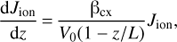 (C.2)
(C.2)
The ENA flux is then given by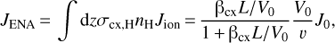 (C.4)
(C.4)
where v is the particle speed and we used βcx = σcxvnH.
Consider next the LOS directed along the infinite heliotail assuming that the plasma speed V is constant and parallel to the LOS. The solution for the ion flux is then (C.5)
(C.5)

The ratio of the ENA flux from the heliotail to the flux from the nose direction is then given by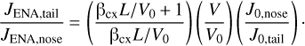 (C.7)
(C.7)
Since βcx decreases with energy, at high enough energy the ENA flux from the heliotail is higher than from the nose direction.
Taking L = 25 AU, nH = 0.1 cm−3 and J0, nose/J0, tail = 2 with V0 = 100 km s−1 for the nose and V = 26 km s−1 for the distant tail, we obtain JENA, tail/JENA, nose = 1.0 at the ENA energy 46 keV and 1.6 at 58 keV (the lowest HSTOF energy for H ENA). The choice of parameters is justified by Voyager 1 (L) and Voyager 2 (V0) observations, by slowing down of the flow in the heliotail from charge exchange with background hydrogen (V), and by nose-to-tail asymmetry of the termination shock (J0, nose/J0, tail). We use the Lindsay & Stebbings (2005) formula for the charge-exchange cross section.
Consider next the case of a time-dependent energetic ion flux J0 at the termination shock. The plasma flow is assumed to remain stationary. The ion flux downstream from the shock in the nose region is given by (C.8)
(C.8)
where τc(z) = − (L/V0)log(1 − z/L) is the convection time from the shock to z. In the tail region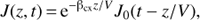 (C.9)
(C.9)
where z/V is the convection time. In the HSTOF energy range the ENA propagation time is short compared to the convection time, so that the time-dependent ENA flux is approximately given by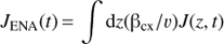 (C.10)
Suppose that the energetic ion flux at the termination shock falls abruptly from the initial value  to zero at the time T. The ENA flux at t < T is given by the time-stationary equations with
  . At t > T it behaves as
 (C.11)
for the nose region, and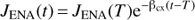 (C.12)
for the tail region. The characteristic decay times (1/(βcx + V0/L) or 1/βcx) are in each case equal to the LOS average of the convection time (τc(z) or z/V) weighted with the energetic ion distribution Jion(z), i.e.,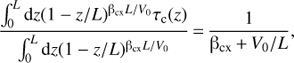 (C.13)
which supports our interpretation of the weighted average of the convection time as a characteristic time for time dependence of the ENA flux.
Appendix D:
Time dependence of the heliospheric ENA flux as observed by IBEX and INCA
The effects on the ENA flux of the solar wind decrease and the subsequent recovery were observed by IBEX and INCA. The results are discussed in recent publications by INCA (Dialynas et al. 2017; Dialynas et al. 2017) and IBEX (McComas et al. 2018) team members.
The evolution of the solar wind ram pressure is reflected in the IBEX yearly ENA maps (McComas et al. 2018, Figs. 1 and 2). Between the years 2005 and 2010 the solar wind ram pressure first falls down, then stays approximately constant between 2010 and 2014, and rapidly increases to a high level during the year 2015. The ENA intensity in the highest energy IBEX channel (4.3 keV) near the nose and ecliptic poles shows similar changes after a delay of 2−3 yr. In particular, the ENA response to the jump in the solar wind ram pressure during the year 2015 starts in late 2016 and becomes prominent in the year 2017. The recovery of the ENA flux is, however, so far confined to the region to the south of the nose, where the energetic particle pressure is high.
The solar wind evolution also affects the energetic ion flux measured by Voyager LECP, causing a drop in intensity, which reached a minimum in the year 2013; this drop was only observed by Voyager 2, since Voyager 1 was then already beyond the inner heliosheath). The INCA energy range overlaps with Voyager LECP, so that the evolution of the ion flux can be directly compared with the INCA ENA flux from the Voyager 1 and 2 directions (Dialynas et al. 2017, Figs. 2 and 3). The time profiles of the ENA flux and the energetic ion flux measured by Voyager 2 agree with each other, both passing through a minimum in the year 2013. A dip in the flux intensity is also found in the time profile of the ENA flux from the anti-nose (tail) direction. In Dialynas et al. (2017) this was proposed as the proof that the heliosphere cannot have an extended tail.
According to our results presented in Sect. 2, a large drop in the HSTOF ENA flux took place before the year 2008 in the HSTOF flank sector. The ENA flux decreases observed by IBEX and INCA occurred three or more years later, so that a common origin with the event observed by HSTOF is, in our opinion, unlikely. Moreover, the changes in the ENA flux noted by IBEX and INCA appeared in the ENA high intensity regions, which, after the year 2005, are outside the field of view of HSTOF. A direct comparison with the HSTOF observations is, consequently, not possible.
Appendix E:
Model of energetic ion distribution in the inner heliosheath
The energetic ion flux of energy E at a chosen point r in the inner heliosheath is calculated as follows.
The termination shock, heliopause, and plasma flow in between are given by a numerical MHD solution. We trace a plasma flow line from r back to the initial point rs on the termination shock. Along this line, we calculate the loss factor e−Λ due to energetic ion neutralization by charge exchange with the hydrogen background, Λ = ∫dsσcx, HvnH, where the integral runs along the flow line, σcx, H is the charge-exchange cross section, v is the ion speed, and nH the neutral H density.
We assume adiabatic evolution of the ion energy in the plasma frame, E ∝ ρ2/3, where ρ is the plasma density. The energetic ion flux f(r) in the plasma frame is then given by f(r, E) = e−Λfs(rs, Es), where fs is the flux at the termination shock and Es is related to E by the adiabatic evolution.
In the calculations reported here we assume a simple power law for fs: fs = CE−1.6 (Hsieh et al. 2010). The coefficient C is taken to scale as the inverse distance from the Sun to the termination shock. Since we are interested only in high energy ions, we disregard the difference between the ion speed in the plasma frame and the speed relative to the neutral H or the observer.
All Tables
All Figures
|
Fig. 1. Ecliptic longitude sectors used for presenting HSTOF data. The four sectors shown on the left are used in the recent studies. The forward sector, which includes the inflow direction of the ISM (eliptic longitude 255°), is also called the “apex”, or the “nose sector”. Early work employed two sectors with the extended “forward sector” that also included the flanks (see right side of figure). |
| In the text | |
|
Fig. 2. Energy-averaged hydrogen ENA flux measurements by HSTOF. The upper panel shows the ENA flux from the flank directions (120° − 210° and 300° − 30° ecliptic longitude sectors). The lower panel shows the flux from the forward sector (210° − 300°), the forward + flanks sector (255° ± 155°), and the heliotail sector (30° − 120° or 50° − 100°). The data are shown as ellipses; the vertical semiaxes represent statistical 1σ deviations and the horizontal axes indicate time intervals. |
| In the text | |
|
Fig. 3. As Fig. 2 but for the case of helium ENA. The upper panel shows He ENA flux from the flank directions (120° − 210° and 300° − 30° ecliptic longitude sectors). The lower panel shows the flux from the forward sector (210° − 300°) and heliotail sector (30° − 120°). |
| In the text | |
|
Fig. 4. Solar wind flux (yearly averages based on OMNI2 data) at 1 AU as a function of time. The time interval starts earlier than the HSTOF observations discussed in this paper because of expected delay between the changes in the solar wind and in the ion distributions in the heliosheath. |
| In the text | |
|
Fig. 5. Schematic view of the heliosphere from the interstellar inflow direction, and, in the upper right part of the figure, the view in the (v, B) plane. The shape of the heliosphere is affected by the interstellar magnetic field. The heliosphere is compressed in the direction perpendicular to the (v, B) plane, but also becomes asymmetric in the (v, B) plane. This effect can lead to the asymmetry between the right and left flanks of the heliosphere, as observed by HSTOF. |
| In the text | |
|
Fig. 6. Tail/apex ENA flux ratio. Crosses show our estimations using the data of IBEX Hi (0.7−4.4 keV, Schwadron et al. 2014) averaged over the period 2009−2013, and INCA (5.2−13.5 and 35−55 keV, Dialynas et al. 2017, Fig. 3a, average over the period 2003−2009). The continuous line indicates the toy model prediction. |
| In the text | |
|
Fig. 7. Estimations of the tail/apex ENA flux ratio as the function of time, based on the results from IBEX (solid lines) and INCA (dashed lines). The following cases are shown: (1) INCA, ENA energy 35−55 keV; (2) INCA, ENA energy 5−13 keV; (3) IBEX, ENA energy 4.3 keV; and (4) IBEX, ENA energy 0.7 keV. In the case of INCA, the ENA flux from the nose direction is replaced by the flux from Voyager 1 or Voyager 2 directions. See the text for detailed description. |
| In the text | |
|
Fig. 8. View of the heliosphere in the ecliptic plane (model 4 in Table 2). The boundaries of the flank regions are shown. The right flank is 1.4 times thicker than the left flank; we use mean thickness in the radial direction. The axes are scaled in AU. The ISM inflow direction is approximately along the vertical axis. |
| In the text | |
Current usage metrics show cumulative count of Article Views (full-text article views including HTML views, PDF and ePub downloads, according to the available data) and Abstracts Views on Vision4Press platform.
Data correspond to usage on the plateform after 2015. The current usage metrics is available 48-96 hours after online publication and is updated daily on week days.
Initial download of the metrics may take a while.