| Issue |
A&A
Volume 618, October 2018
|
|
|---|---|---|
| Article Number | A141 | |
| Number of page(s) | 15 | |
| Section | Stellar atmospheres | |
| DOI | https://doi.org/10.1051/0004-6361/201630352 | |
| Published online | 22 October 2018 | |
An empirical recipe for inelastic hydrogen-atom collisions in non-LTE calculations⋆
1 Laboratoire Univers et Particules de Montpellier, Université de Montpellier, CNRS, UMR 5299 Montpellier, France
2 Joint Institute for Nuclear Astrophysics, Center for the Evolution of the Elements, East Lansing, MI 48824, USA
3 Kavli Institute for Astrophysics and Space Research, Massachusetts Institute of Technology, Cambridge, MA 02139, USA
e-mail: This email address is being protected from spambots. You need JavaScript enabled to view it.
4 Institut d’Astronomie et d’Astrophysique, Université Libre de Bruxelles, CP 226, Boulevard du Triomphe, 1050 Brussels, Belgium
5 Department of Physics and Astronomy, Notre Dame University-Louaize, PO Box 72, Zouk Mikaël, Lebanon
6 Université Côte d’Azur, Observatoire de la Côte d’Azur, CNRS, UMR7293, CS 34229, 06304 Nice Cedex 4, France
Received:
23
December
2016
Accepted:
27
August
2018
Abstract
Context. Determination of high-precision abundances of late-type stars has been and always will be an important goal of spectroscopic studies, which requires accurate modeling of their stellar spectra with non-local thermodynamic equilibrium (NLTE) radiative transfer methods. This entails using up-to-date atomic data of the elements under study, which are still subject to large uncertainties.
Aims. We investigate the role of hydrogen collisions in NLTE spectral line synthesis, and introduce a new general empirical recipe to determine inelastic charge transfer (CT) and bound-bound hydrogen collisional rates. This recipe is based on fitting the energy functional dependence of published quantum collisional rate coefficients of several neutral elements (BeI, Na I, Mg I, Al I, Si I and Ca I) using simple polynomial equations.
Methods. We perform thorough NLTE abundance calculation tests using our method for four different atoms, Na, Mg, Al and Si, for a broad range of stellar parameters. We then compare the results to calculations computed using the published quantum rates for all the corresponding elements. We also compare to results computed using excitation collisional rates via the commonly used Drawin equation for different fudge factors, SMH, applied.
Results. We demonstrate that our proposed method is able to reproduce the NLTE abundance corrections performed with the quantum rates for different spectral types and metallicities for representative Na I and Al I lines to within ≤0.05 dex and ≤0.03 dex, respectively. For Mg I and Si I lines, the method performs better for the cool giants and dwarfs, while larger discrepancies up to 0.2 dex could be obtained for some lines for the subgiants and warm dwarfs. We obtained larger NLTE correction differences between models incorporating Drawin rates relative to the quantum models by up to 0.4 dex. These large discrepancies are potentially due to ignoring either or both CT and ionization collisional processes by hydrogen in our Drawin models.
Conclusions. Our general empirical fitting method (EFM) for estimating hydrogen collision rates performs well in its ability to reproduce, within narrow uncertainties, the abundance corrections computed with models incorporating quantum collisional rates. It performs generally best for the cool and warm dwarfs, with slightly larger discrepancies obtained for the giants and subgiants. It could possibly be extended in the future to transitions of the same elements for which quantum calculations do not exist, or, in the absence of published quantum calculations, to other elements as well.
Key words: atomic processes / line: formation / stars: abundances / stars: atmospheres / stars: late-type
Tables A.1–A.4 are only available at the CDS via anonymous ftp to cdsarc.u-strasbg.fr (130.79.128.5) or via http://cdsarc.u-strasbg.fr/viz-bin/qcat?J/A+A/618/A141
© ESO 2018
1. Introduction
In the era of large-scale surveys tracing the history of stellar populations (e.g., RAVE, Steinmetz et al. 2006; APOGEE, Allende Prieto et al. 2008; Gaia-ESO, Gilmore et al. 2012, etc.), there is an important need for high-accuracy, detailed chemical composition determinations. Most stellar spectroscopic analyses adopt the assumption of local thermodynamic equilibrium (LTE). This assumption is however not always valid, especially when collisions are not frequent enough to ensure excitation and ionization equilibrium of the atomic populations. Collisions in cool stellar atmospheres are mainly due to electrons and hydrogen atoms. Although electrons have larger thermal velocities than hydrogen atoms by a factor of approximately 43, they can be less numerous than hydrogen atoms in late-type stellar atmospheres (Lambert 1993). In fact, in low-metallicity stars, electron densities are much lower (by the order of 10−4) and non-LTE (NLTE) effects are expected to grow stronger, as well as in giants’ and supergiants’ rarefied atmospheres (Thévenin & Idiart 1999; Asplund 2005; Lind et al. 2011).
NLTE modeling requires a great deal of atomic data for each element under consideration. Large experimental and theoretical efforts have been devoted to measuring and calculating energy levels, ɡf-values, and broadening parameters (e.g., Anstee & O’Mara 1995; Castelli & Kurucz 2010; Peterson & Kurucz 2015; Barklem et al. 2015), for example. Hydrogen collision rates remain, however, a major source of uncertainty in NLTE calculations for cool stars (Asplund 2005; Barklem et al. 2010). Quantum mechanical collision rates have been computed for a small number of atoms over the past decade including Be (Yakovleva et al. 2016), Na (Barklem et al. 2010), Mg (Belyaev et al. 2012; Guitou et al. 2015), Al (Belyaev 2013), Si (Belyaev et al. 2014), K (Yakovleva et al. 2018), Ca (Barklem 2016; Mitrushchenkov et al. 2017; Belyaev et al. 2017), Mn (Belyaev & Voronov 2017) and Rb (Yakovleva et al. 2018).
In the absence of such calculations for other atoms, the Drawin approximation (Drawin 1968, 1969a,b; Steenbock & Holweger 1984; Lambert 1993) is customarily used to estimate the collisional cross-sections. This approximation was originally derived from the classical Thomson (1912) e− + atom ionization rate equation. The Drawin equation has been applied to allowed bound-bound (b−b) and ionization bound-free (b−f ) transitions, where it has been shown to overestimate the collisional rates by orders of magnitude (Barklem et al. 2010). A fudge-factor, SH, is usually applied in most studies to try to compensate for this overestimation. Several SH-factors have been proposed for different atoms. As an example, for Al I, values between 0.002 and 0.3 have been suggested (e.g., SH = 0.1, Mashonkina et al. 2016b; SH = 0.002, Gehren et al. 2004; Baumueller & Gehren 1996, 1997; SH = 0.1, Andrievsky et al. 2008; and SH = 0.3, Steenbock & Holweger 1992).
Recently, charge transfer (CT) rates, corresponding to the ion-pair production and mutual-neutralization processes: A + H ⇋ A+ + H− (A denoting an atom other than H), have been shown to be larger than the b−b rates (Barklem et al. 2010). During a collision, the valence electron of the atom A has the potential to tunnel to the H atom at an avoided crossing. Later, at a different avoided crossing, it may tunnel back to another covalent molecular level, leading to a different final state of the atom A, and an excitation or de-excitation of the atom. The electron may also stay with the H atom, leading to an ion-pair production. The former process is more likely to have a small-valued cross-section as it implies passing two avoided crossings, the higher-lying being passed with a small transition probability (Barklem et al. 2011). The CT rates therefore play an important, and in some cases, even dominating role in the collisional processes (Lind et al. 2011; Osorio et al. 2015; Guitou et al. 2015) and should therefore be included in NLTE calculations. In Ezzeddine et al. (2016), we used the Drawin formula to estimate CT rates, in the absence of any other approximation. We defined two scaling-factors SH for b−b and b−f, and SH(CT) for CT rates for Fe I transitions, and tried to calibrate them using benchmark star spectra (α Cen A, HD 140283 and the Sun). Our method used a χ2-minimization of differences between observed and calculated iron-line equivalent widths (EWs) for different sets of SH and SH(CT). We could not find a combination of SH and SH(CT) that would work for the three stars. This difficulty of the Drawin formula to reproduce the behavior and magnitude of hydrogen collision rates, independent of the stellar and atomic models used, calls for another approach, as long as no quantum calculation are available.
This is the motivation for our work, which introduces an empirical fitting method (EFM) to estimate the hydrogen collision rates for both b−b and CT processes. It is based on the observation that the existing well determined quantum rates all behave similarly, and can be described with simple fitting functions. Recent studies by Belyaev & Yakovleva (2017b,a) also used such observations to derive general recipes for estimating neutral and ionic hydrogencollisional rates forb−band CT rate coefficients based on a simplified approach of the Landau-Zener R-matrix model. Their results were published during the course and after the submission of this work. In their recipes they estimate b−b and CT reduced rate coefficients of dominant transitions as a function of collision energies and statistical probabilities of the relevant atomic levels, which they tested on K for neutral rates and Ba for ionic rates. We performed comprehensive tests of our method on four atoms belonging to different groups in the periodic table for which quantum rates have been calculated, namely Na, Mg, Al and Si. We built model atoms for each of these elements and implemented different recipes for H collisions, including our empirical fitting recipe, published quantum rates as well as rates computed using the Drawin equation. We then use them to perform and compare NLTE calculations for a large range of stellar parameters.
This article is divided as follows. In Sect. 2, we introduce the empirical fitting method and its application to estimate the hydrogen collision rates for both CT and de-excitation rates. In Sect. 3, we put our method to the test on four elements for which we built new model atoms. In Sect. 4, we compare the line profiles and NLTE abundance corrections obtained by the different models and present our results. Finally, conclusions are presented in Sect. 6.
2. Introducing the general empirical recipe
Our empirical recipe to estimate the hydrogen collisional rates for both CT and (de-)excitation processes is motivated by the similar behavior of the quantum-mechanical hydrogen collision rates for several neutral species of atoms including Be (Yakovleva et al. 2016), Na (Barklem et al. 2010), Mg (Belyaev et al. 2012; Guitou et al. 2015), Al (Belyaev 2013), Si (Belyaev et al. 2014), K (Yakovleva et al. 2018), Ca (Barklem 2016; Mitrushchenkov et al. 2017; Belyaev et al. 2017), Mn (Belyaev & Voronov 2017) and Rb (Yakovleva et al. 2018).
This similarity is shown in Fig. 1, where the CT rates at T = 6000 K are shown for these nine atoms.
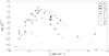 |
Fig. 1. CT rate coefficients (in logarithmic scale), log QCT, as a function of inverse transition energies |

We chose to plot the logarithm of the Maxwellian averaged cross-sections Q = QCT (cgs units) as a function of inverse transition energy 1/ΔE (eV−1), where ΔE = Eup − Elow is the energy difference between the upper and the lower level of the transition. As the upper state consists of H− + A+, its energy is the iron ionization potential decreased by 0.754 eV, the H− electron affinity. Figure 1 shows that the rates of all nine elements have a peak value of QCT ∼ 10−7 cm3 s−1 arising at 1/ΔE between 0.5 and 1eV−1. The empirical fitting method (EFM) is based on fitting these rates as a function of ΔE using simple general recipes, as explained in detail below. The hydrogen rate coefficients for K, Mn and Rb were published during the course of this work, and were thus excluded from the fitting process and analysis hereafter. However, their rates as shown in Fig. 1, behave similarly to the other six atoms. Their exclusion from the analysis should therefore not affect the final results of this work.
2.1. Charge transfer rates
Figure 2 shows the fits to the logarithm of the mutual-neutralization (downward CT) rate coefficients, log QCT, of Be I, Na I, Mg I, Al I, Si I and Ca I from Yakovleva et al. (2016), Barklem et al. (2010), Belyaev et al. (2012, 2014, 2017), Guitou et al. (2015), Belyaev (2013), respectively.
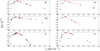 |
Fig. 2. CT rate coefficients log QCT at T = 6000 K, for Be I, Na I, Mg I, Al I, Si I and Ca I (filled triangles) from the quantum calculations of Yakovleva et al. (2016), Barklem et al. (2010), Belyaev et al. (2012, 2014, 2017), Guitou et al. (2015), Belyaev (2013), respectively. The polynomial fits as per the EFM (dashed red lines) are also displayed on the plots. |
We only include the rates at T = 6000 K, as they show a similar behavior at other temperatures. The temperature dependence is discussed further below.
We chose an inverse energy scale representation to allow simple linear fits of most of the data. Rates lying more than four orders of magnitude below the peak were ignored, as such rates will not contribute significantly to the NLTE calculations (Barklem et al. 2011). We are thus able to describe the CT rate coefficients, log QCT, of all six elements as a function of 1/ΔE with the following recipe:
 (1)
(1)
where a1 and a2 are the positive and negative slopes of the linear fits, respectively, and Qmax is the maximum peak rate at  . The temperature dependence of the CT fitting parameters a1, a2,
  and log Qmax were also investigated. As an illustration, the temperature dependence is shown for the case of Si in the upper panels of Fig. 3. The coefficient a1 is roughly linearly temperaturedependent, while log Qmax depends linearly on log T. The coefficients a2 and
  do not vary significantly with temperature. It follows that a1 and log Qmax can be written as a function of temperature T as:
 (2)
(2)
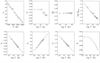 |
Fig. 3. Temperature dependence plots for the CT rate fitting coefficients a1, a2, |

Coefficients a11, a10, α and log Q0, as well as a2 and 1/ΔE0 obtained for the six elements are shown in Table 1. The average position in energy of the maximum rate, log Q0 = −7.35 ± 0.37, is well defined at 1/ΔE0 = 0.73 ± 0.10 eV−1, with a temperature exponent α = −0.35 ± 0.22. More scatter is found for the a coefficients, with an average a10 = 5.7 ± 3.7, a11 = −1.1 ± 0.9, and a2 = −2.4 ± 1.2. The temperature dependence is weak for all six elements, with a variation of log QCT by a factor of about 1.5 in the temperature range 3000−10 000 K. The slope at small energy difference, a2, is independent of the temperature, and at larger energy difference a1 decreases by less than 15%. The effects of the temperature dependence of the rates on NLTE abundance calculations are further discussed in Sect. 5.
CT and b−b hydrogen collision rate fitting coefficients obtained for the neutral species of Be, Na, Mg, Al, Si and Ca.
For the six elements, the functional dependencies on energy and temperature of the rates, and hence of the fitting coefficients, are very similar; the peak value of the CT rates, their position, and even the slopes with energy are quite close. The reason for this similarity in the behavior of the rates is the presence of avoided crossings of the AH molecular potentials and the A+H− ionic potential. The peaks shown for all the atoms at approximately the same transition energies correspond to transitions occurring at optimal internuclear distances (Barklem et al. 2011; Barklem 2018).
2.2. De-excitation (b−b) rates
The de-excitation (downward b−b) rates for Be I, Na I, Mg I, Al I, Si I and Ca I show a larger scatter than CT rates, with many more transitions; they show a general decrease with increasing transition energy (Fig. 4). The rates at large energy differences are in general much smaller than the rates for levels lying close to each other. An exception is Ca for which the collisional rates between some close lying levels are extremely small. The collisional b−b rates for all six elements can be best fit as a function of ΔE using a third degree polynomial:
 (3)
(3)
In addition, b3, b2 and b1 are linearly dependent on log T, while b0 does not vary much with temperature, as is demonstrated for Si in the lower panels of Fig. 3. This allows us to write the b−b fitting parameters as:
 (4)
(4)
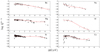 |
Fig. 4. De-excitation rate coefficients log Qb−b at T = 6000 K (in logarithmic scale) for Be I, Na I, Mg I, Al I, Si I and Ca I from the quantum calculations of Yakovleva et al. (2016), Barklem et al. (2010), Belyaev et al. (2012, 2014, 2017), Guitou et al. (2015), Belyaev (2013), respectively. Their corresponding polynomial fits (dashed red lines) are also shown. |
The b parameters for the six elements are listed in Table 1. The b0 coefficient, that is, the asymptotic value of log Qb−b for Δ E = 0 eV, lies between −9.7 and −11.3, with an average log Qb−b = −10.40 ± 0.9. The other polynomial fitting coefficients for the b−b rates (b31, b30, b21, b20, b11 and b10) vary more severely from one atom to the next than for the CT rates. This is due to the large number of b−b transitions of differing character. It is also probably affected by the dependency of the rates on a double tunneling of the electron between the ionic and the valence states, as explained in Sect. 2.1. Again, the b−b fitting coefficients’ temperature dependence and their effects on the NLTE abundance calculations are tested in Sect. 5.
3. Testing the empirical fitting method on Na, Mg, Al and Si atoms
The similar behavior of the CT and b−b collisional quantum rates of the six atoms described above prompted us to develop our empirical fitting method to estimate hydrogen collisional rates in NLTE abundance calculations, whenever quantum computations are not available. To further put our proposed method to the test, we performed NLTE abundance calculations for four of the six atoms described above, Na, Mg, Al and Si. These elements belong to four different groups in the periodic table: alkali metals (Na), alkaline earth metals (Mg), post-transition metals (Al) and metalloids (Si). The other two elements, Be and Ca also belong to the alkaline earth metals and are therefore expected to behave similarly to Mg.
For that purpose, we built model atoms for Na, Mg, Al and Si, which were used to compute NLTE calculations. We then compared NLTE line profiles and abundance corrections determined for representative lines of each element using hydrogen collisional rates implemented from (i) published quantum rates and (ii) our empirical fitting method using the fitting coefficients derived for each element from Table 1. For comparison, we also performed additional calculations for each element using hydrogen collisional rates computed using the classical Drawin equation (Drawin 1968, 1969a) and adopting different fudge factors: (iii) SH = 0.1 and (iv) SH = 1.0 for Na I, Mg I, Al I and Si I, as well as (v) SH = 0.002 for Al I as recommended by Gehren et al. (2004) and Baumueller & Gehren (1996, 1997). The calculations were tested on a grid of stellar atmospheric parameters corresponding to typical FGK stars. The model atoms and input model atmospheres used, as well as a detailed explanation of the tests performed to compare the results for each method, are presented below.
3.1. Model atoms for Na, Mg, Al and Si
The atoms for Na, Mg, Al and Si used in the tests of the NLTE calculations were homogeneously built by the code FORMATO2.0 (Merle et al., in prep.) using atomic data adopted from different atomic databases and references as described below.
3.1.1. Energy levels
Fine structure energy levels of the neutral and first ionized species of each element, as well as the mean ground level of the second ionized species, were included in each model atom. Fine-structure energy levels were extracted from the NIST1, VALD32, Kurucz atomic line3 and The Opacity Project (TOPBASE4) databases and the references therein. The number of fine-structure levels as well as the source databases used for each species of each element are listed in Table 2.
Atomic databases and references used for the sources of energy levels and radiative and collisional b−b and b−f transitions used for each species in our model atoms for Na, Mg, Al and Si.
3.1.2. Radiative transitions
Line data for radiative transitions between the energy levels were extracted from the NIST, VALD3 and Kurucz atomic line databases. The oscillator strengths were adopted from the corresponding references therein. The Van der-Waals hydrogen collisional broadening coefficients were calculated using the ABO theory (Anstee & O’Mara 1995; Barklem & O’Mara 1997; Barklem et al. 1998) for available transitions, and otherwise using the Unsöld approximation (Unsold 1955), enhanced by species-dependent fudge factors as recommended by Gustafsson et al. (2008).
All levels in the model atoms were also coupled to the first ionized species’ ground levels via bound-free (b−f ) radiative (photoionization) transitions. The b−f photoionization tables were extracted from the TOPBASE which were calculated using the close-coupling approximation and the R-matrix method. Due to the large number of points in the tables and the sharp resonance peaks in the data, the cross-sections were smoothed and re-sampled before being implemented in the atoms. For transitions for which no photoionization table exists, Kramer’s hydrogenic approximation (Travis & Matsushima 1968) was used to calculate the threshold cross-sections. Details on the number of b−b radiative transitions used for each atom, as well as the database sources used for each atom, are listed in Table 2.
3.1.3. e− collisional transitions
All levels in the model atoms are coupled via inelastic collisions with electrons. Quantum calculations for effective collisional strengths Υe− for electron collisions were implemented for the Mg I model atom following Merle et al. (2015). For transitions where no quantum data are available, classical and semi-classical approximations were used. For allowed b−b and ionization by electron collisional transitions, the Seaton (1962a) impact parameter approximation was used. For forbidden b−b transitions, Seaton (1962b) approximation was used with a collisional strength of Υe− = 1, as recommended for neutral atoms by Allen (1973).
3.1.4. H collisional transitions
Inelastic hydrogen collisions were included as follows: different model atoms were built for each element using different recipes for b−b and CT (whenever possible) hydrogen collision rates implemented for the neutral species, using: (i) published quantum rates for b−b and CT collisions (hereafter denoted as the QM models), (ii) our empirical fitting method with fitting coefficients from Table 1 for b−b and CT collisions (hereafter denoted as the EFM model), (iii) Drawin equation for b−b collisions with SH = 0.1 and (iv) Drawin equation for b−b collisions with SH = 1.0 (denoted as the DRW, SH = 0.1 and DRW, SH = 1.0 models, respectively). For Al, an additional atom was built implementing H rates using the Drawin equation for b−b collisions with SH = 0.002 (denoted as the DRW, SH = 0.002).
For a better comparison of the models, only the transitions for which quantum data are available in the QM models for each element have been implemented in the corresponding EFM models. For the DRW models, we ignored ionization collisions by hydrogen in the DRW models (Steenbock & Holweger 1984), which have been commonly implemented in previous NLTE calculations (e.g., Gehren et al. 2004; Mashonkina 2013).
In addition to the previous restriction, DRW b−b rates were only included for the collisional transitions with allowed radiative counterparts (i.e., with calculated oscillator strengths). For the first ionized species (considered dominant in all four elements in FGK-type stars), the Drawin approximation was used.
3.2. Stellar parameters and model atmospheres
To test our empirical fitting method, we perform NLTE calculations for each of the QM, EFM and DRW model atoms of each element for a grid of stellar parameters corresponding to typical FGK-type stars. The stellar atmospheric parameters used in the grid (effective temperature Teff; surface gravity log ɡ; metallicity [Fe/H]; and microturbulent velocity, ξt) are shown in Table 3, and were chosen to correspond to three stellar evolutionary stages: giants (log ɡ = 2.5), sub-giants (log ɡ = 3.5) and dwarfs (log ɡ = 4.5). Typical ξt values were adopted for each log ɡ value as shown in Table 3, such that ξt = 2.0 was chosen for the giants, ξt = 1.8 for the sub-giants and ξt = 1.5 for the dwarfs. Corresponding Teff values were adopted for each evolutionary stage following the Teff − log ɡ diagram from Heiter et al. (2015) for the Gaia benchmark FGK stars (see their Fig. 8). Teff = 4500 K was used for log ɡ = 2.5, Teff = 4500 K and 5500 K were used for log ɡ = 3.5, and Teff = 4500 K, 5500 K, and 6500 K were used for log ɡ = 4.5. For each log ɡ/ Teff combination, four metallicity values were adopted from [Fe/H]=−3.0 to [Fe/H]=+0.0 in steps of Δ = 1.0 dex. NLTE calculations were thus performed for a total of 24 atmospheric models for each atomic model of each element, giving a total of 96 models for each. One dimensional (1D) LTE MARCS model atmospheres (Gustafsson et al. 2008) were interpolated to the corresponding atmospheric parameters using the interpolation routine interpol_marcs.f written by Thomas Masseron5.
Grid of stellar parameters for which the NLTE calculations for all atoms were performed.
3.3. NLTE methods
The NLTE radiative transfer code MULTI2.3 (Carlsson 1986, 1992) was used to compute the level populations and the line EWs. An edited version of MULTI2.3 was used6 where CT collisional rates were computed from the input ion-pair production (downward CT) rate coefficients implemented in the model atoms, and the H− number densities determined using the Saha equation (Saha 1921). Background line opacity files excluding lines of the corresponding elements (e.g., Na background lines were excluded from the calculations for the Na atoms) were included in the MULTI2.3 calculations to account for line blanketing effects. The opacity files were computed for each model metallicity ([Fe/H]) and microturbulent velocity using the MARCS opacity sampling routines. We computed the corrections for each line, defined as the difference between the NLTE and LTE abundances that corresponds to the same EW, Δ log ε = log ε(NLTE) − log ε(LTE).
To determine the abundance corrections, we first computed the NLTE and LTE curve-of-growth from five abundance points for each model atom for the 24 atmospheric parameters defined in the grid in Sect. 3.2. The abundance points were varied around the central abundance value adopted in each model, in steps of Δ = ±0.3 dex each time. For models where NLTE abundance corrections > ± 0.6 dex were obtained, additional abundance points were added up to ±1.2 dex from the central abundance to avoid extrapolation. The abundance corrections between the NLTE and LTE curves of growth were derived by interpolating the NLTE curve of growth to the corresponding LTE EW of the median abundance, considered as the reference for each model. The interpolation method from Steffen (1990) was used. Corrections were considered for all lines except for those with EW < 0.5 mÅ. The NLTE corrections determined for the considered lines of Na I, Mg I, Al I and Si I at the corresponding Teff/log ɡ/[Fe/H] values for all different model atoms described in Sect. 3.1 are shown in Tables A.1–A.4.
4. Results
An important test of the EFM is for its ability to reproduce the line profiles and NLTE abundance corrections computed using the QM, for a range of stellar parameters. We represent below the comparisons of such results obtained with the two collision models for representative lines of Na I, Mg I, Al I and Si I. We also compare the line profiles and abundance correction differences obtained between the Drawin models (DRW) to those of the QM.
The aim of this study is to solely compare the NLTE abundance corrections obtained from different implementations of recipes for hydrogen collision rates in the atomic models using only the same H collisional transitions as those published for the quantum models. We therefore do not present detailed comparisons to observations or physical interpretation of the obtained NLTE corrections. We refer the reader to previous detailed NLTE studies for such interpretations such as, but not limited to, Mashonkina et al. (2000), Andrievsky et al. (2007), Lind et al. (2011) for Na I, Merle et al. (2011), Mashonkina (2013), Osorio et al. (2015), Bergemann et al. (2017) for Mg I, Mashonkina et al. (2016a), Nordlander et al. (2017) for Al I and Shi et al. (2008), Bergemann et al. (2013), Mashonkina et al. (2016a) for Si I.
4.1. Line profile comparisons
We compare the NLTE line profiles computed using the different collision models. We choose to show in Fig. 5, the line profiles computed using the QM, EFM, DRW, SH = 0.1 and DRW, SH = 1.0 models for the lines at Na I 6154 Å, Mg I 4730 Å and Si I 5772 Å, in addition to the DRW, SH = 0.002 model for Al I 6696 Å. The lines are shown at Teff = 4500, log ɡ = 2.5 and for both [Fe/H] = +0.00 and −3.00, respectively. We compare the lines computed with the different collision models relative to the QM, by calculating the χ2 difference between each (shown in Fig. 5). The strengths and shapes of the lines computed using the EFM are able to efficiently reproduce those of the QM for the four atomic species. For the solar case ([Fe/H] = +0.00), all collision models compare similarly well relative to the QM. The Na I 6154 Å, Mg I 4730 Å, and Al I 6696 Å lines computed with DRW models have slightly weaker cores than the QM and EFM models. As expected, the lines become much weaker for the extremely metal-poor case ([Fe/H] = −3.00) as compared to the solar one. The line profiles computed using the EFM and QM show very good agreement for the metal-poor stars, while those computed with the DRW models for Na I, Mg I, and Al I have weaker cores and wings. The Si I 5772 Å QM line can be best reproduced with the DRW, SH = 1.0 model for both [Fe/H] values, with the EFM models being slightly stronger. We obtained similar results for other lines of Na I, Mg I, Al I and Si I as well.
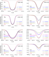 |
Fig. 5. Line profiles of Na I 6154 Å, Mg I 4730 Å, Al I 6696 Å and Si I 5772 Å computed using different hydrogen collision models: QM (black lines), EFM (red lines), DRW, SH = 0.1 (blue lines), DRW, SH = 0.1 (olive lines) and DRW, SH = 0.002 for Al I (magenta lines). The lines were computed at Teff = 4500, log ɡ = 2.5 and for two metallicities, [Fe/H] = +0.00 (left panels) and [Fe/H] = −3.00 (right panels). The χ2 differences obtained between each model relative to the QM are shown on the plots. |
4.2. NLTE abundance correction comparisons
We then investigate the ability of the EFM to reproduce the results of the QM models by determining the NLTE abundance correction differences between the two collision models for representative lines of Na I (7 lines), Mg I (8 lines), Al I (6 lines) and Si I (6 lines) listed in Tables A.1–A.4. This was done for the set of stellar parameters defined by our grid (Table 3).
4.2.1. Sodium
The overall differences in abundance corrections obtained between the QM and other collision models are shown for Na I in the box plots of the upper left panels of Fig. 6. Left-hand panels display box plots of the abundance correction differences obtained between the QM and the corresponding collision model including the considered seven Na I lines at four different [Fe/H] values (i.e., a total of 28 lines). This is shown for different spectral types defined by the corresponding stellar parameters: cool dwarfs (Teff = 4500, log ɡ = 4.5), cool giants (Teff = 4500, log ɡ = 2.5), subgiants (Teff = 5500, log ɡ = 3.5), and warm dwarfs (Teff = 6500, log ɡ = 4.5). Right-hand panels show similar plots for the differences obtained at different metallicities including all six considered Teff/log ɡ combinations (i.e., a total of 42 lines). On average, the Na I abundance corrections computed with the EFM models are in agreement with those computed using the QM collisions to within <0.03 dex, at different metallicities and spectral types. Approximately 50% of the lines (defined by the upper and lower limits of the box plots) lie within ±0.02 dex of the QM. Slightly larger differences, but within 0.04 dex, are obtained for the cool dwarfs and the [Fe/H] = −3.00 models. Ninety percent of all lines (defined by the upper and lower limits of the box whiskers) lie within ±0.05 dex of the reference QM values. Outlier models (∼1% of the lines) show slightly larger differences, up to 0.08 dex. These correspond particularly to the Na I lines at 6160 Å and 6154 Å for the cool dwarf case at [Fe/H] = −3.0. The overall differences between the QM and the Drawin models are also displayed. The abundance corrections obtained by the DRW, SH = 0.1 models are less discrepant relative to the QM than the SH = 1.0. Corrections computed with both DRW models overestimate the QM results by up to 0.10 dex for SH = 0.1 and 0.15 dex for SH = 1.0, especially for the cool dwarfs, independent of metallicities. The effect of collisions in Na I NLTE abundance corrections was tested in detail by Lind et al. (2011). They found that the CT hydrogen collisions can be important for cool dwarf models. While our DRW models differ from theirs in terms of ignoring ionization collisions by H, we find similar results to their findings for the cool dwarfs, where the largest differences in abundance corrections between the QM and DRW models are obtained, up to 0.20 dex. In general, our results show that our DRW models seem to be able to best reproduce the QM results for the considered Na I lines for the warm and solar [Fe/H] stars to within <0.05 dex. This is also in agreement with the results from Lind et al. (2011), who reported negligible hydrogen collision effects on the abundance corrections for solar-type models.
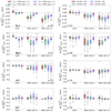 |
Fig. 6. Box plots showing the overall NLTE abundance correction differences obtained between models computed with the QM rates and those computed with the EFM, DRW, SH = 0.1 and DRW, SH = 1.0 rates (for Al I, we choose to show results for DRW, SH = 0.002 instead of DRW, SH = 1.0). Boxes in each panel display the differences obtained from representative lines of Na I, Mg I, Al I and Si I (shown in Table A.1) for the corresponding stellar parameters of cool dwarfs (in red), cool giants (in green), subgiants (in blue) and warm dwarfs (in magenta) in the left-hand panels. Right-hand panels show the same plots for different metallicities. The number of lines, n, used in each box plot is displayed. Black solid lines show the median values obtained for each model and each atom, colored boxes represent 50%, and whisker edges 90% of the lines. Gray circles show the remaining outlier lines. |
In Figs. 7 and 8, we show similar comparisons for four individual Na I lines at 5895 and 8183 Å, and at 5682 and 6154 Å, respectively, as a function of [Fe/H], for the cool giants, cool dwarfs, and warm dwarfs. The corrections determined using the EFM models for the four Na I lines are within <0.05 dex of the QM, for the set of stellar parameters considered. We also show for reference, on the same figures, the NLTE abundance corrections obtained by the QM models (denoted by  ). The differences between the QM and EFM models are typically smaller than
  , except for when
  where the differences become comparable. The corrections computed by the Drawin models, on the other hand, show larger discrepancies (>0.05) relative to the QM for the cool star models at lower metallicities ([Fe/H] ≤−2.0). The discrepancies are smaller for DRW, SH = 0.1 and are of the order of ∼0.1 dex relative to the QM. They are, however, in better agreement to within <0.05 for the warmer stars and solar-metallicity models. We also show the correction differences between the QM and EFM models (in absolute values) for Na I 5682 Å as a function of Teff, log ɡ, and [Fe/H] defined by the contour surface plots of Fig. 9. Values of
  (also in absolute values) are represented with the line iso-contours on the same figure. Again, the EFM models are able to efficiently reproduce the QM abundance corrections to within <0.05 dex, especially for the higher-gravity models for all four [Fe/H] considered. The correction differences (shaded contours) between the QM and EFM models are typically smaller than
  (iso-contours), which can reach up to ∼0.15 dex for this line at log ɡ = 2.5 for [Fe/H] = −1.0 and [Fe/H] = +0.0, respectively.
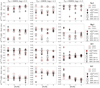 |
Fig. 7. Abundance correction differences obtained between the QM and the corresponding EFM (empty circles), DRW, SH = 0.1 (empty squares) and DRW, SH = 0.1 collision models (empty triangles), as well as DRW, SH = 0.002 for Al I, (empty stars) for select Na I, Mg I, Al I and Si I lines, as a function of [Fe/H]. This is shown for the cool giants and dwarfs (left-hand and middle panels), as well as the warm dwarfs (right-hand panels) stellar parameters. The NLTE abundance corrections obtained by the QM models are also shown (filled diamonds), for comparison. |
4.2.2. Magnesium
Similar to Na I, we compare the abundance correction differences obtained between the EFM and QM models for eight Mg I lines at 4571 Å, 4702 Å, 4730 Å, 5172 Å, 5183 Å, 5528 Å, and 5711 Å and the NIR line at 11828 Å. Results for 5528 Å and 11828 Å are displayed in Fig. 7, while those for 4571 Å and 5172 Å are shown in Fig. 8 as a function of stellar parameters. The Mg I abundance corrections determined with the EFM are able to reproduce those of the QM to within <0.02 dex for the cool dwarfs and <0.05 dex for the cool giants. Larger discrepancies exist for the subgiant (<0.12 dex) and warm dwarf cases (<0.1 dex). This is also shown in Fig. 6 upon considering a total of 32 Mg I lines for each spectral type (left panels) and 48 lines for each metallicity (right panels). The overall differences are smaller for the cool stars. They become slightly larger toward the Teff = 5500 K subgiants, where the largest discrepancies (∼ 0.3 dex) are obtained for Mg I 5711 Å at [Fe/H] = −3.00 (shown by the outlier points on Fig. 6). The same behavior is obtained for the four metallicities, with the smallest differences being obtained for the solar values.
For the warm dwarf models, the largest discrepancy of 0.15 dex is obtained for the Mg I line at 5172 Å, a component of the Mg I b triplets (5167, 5172, 5183). Being very strong at this warm temperature (Teff = 6500 K), this line is, however, rarely used in abundance analyses. The NLTE abundance corrections obtained by the QM models are negligible for the cool stars (< 0.05 dex). The differences between the QM and our DRW models are more significant for the cool giants and subgiants, with larger discrepancies obtained for SH = 0.1. In these cases, the abundance correction differences between the DRW and QM models are up to 0.25 dex, with some lines even deviating up to 0.40 dex. We compared our results to those obtained by Mashonkina (2013) for the same Mg I lines and similar stellar parameters. Our results show that the absolute correction differences between the QM and DRW models are over-estimated as compared to Mashonkina’s. For example, they obtain 0.02 dex and 0.03 dex absolute differences for the warm dwarfs at [Fe/H] = −1.00 between the QM and DRW, SH = 0.1 models for the Mg I lines 5172 Å and 4571 Å, respectively. We, on the other hand, obtain absolute differences of 0.17 dex and 0.08 dex, respectively, for the same lines and stellar parameters. Our values agree better for the 5528 Å line, with 0.01 dex difference between our results. Similar discrepancies are obtained for the cool giants. Such differences between both our studies could either be due to (i) neglecting ionization collisions in our DRW models, which leads to stronger absolute NLTE corrections as compared to her results, or (ii) implementing a smaller number of H b−b collisional transitions in our DRW models as compared to her model, where forbidden transitions and those for which no QM rates existed were excluded. The Mg I line abundance correction dependencies on hydrogen collisions were explicitly investigated by Osorio et al. (2015). They found that these dependencies varied from line to line as the level populations in the Mg I atom were affected differently by the different H collisional processes. Particularly, the CT rates were found to affect some lines more than others (such as the 5528 Å line), whereas excitation b−b collisional rates were found to be more important for others (such as for the 8806 Å line). Similar to our results for Na I, our results for the DRW models seem to best be able to reproduce the QM abundances for Mg I lines at the solar metallicities.
4.2.3. Aluminum
For Al I, we consider six representative Al I lines, namely, the doublet lines at 6696–6698 Å, the optical lines at 7836 Å and 8773 Å, as well as the NIR lines at 13123 Å and 16718 Å. The abundance corrections obtained by the EFM efficiently reproduce those of the QM to within 0.03 dex. This is shown for Al I 6696 Å and 8773 Å in Fig. 7, and for 13123 Å and 7836 Å in Fig. 8. Slightly larger discrepancies of up to 0.05 dex are obtained for the warm dwarfs. They are, however, comparatively smaller than the reference QM NLTE abundance corrections which can reach up to 0.6 dex for the doublet line at 6696 Å at [Fe/H] = −3.0.
Overall, the corrections derived with the EFM for all our considered Al I lines perform well as compared to the QM (within ±0.03 dex) for different stellar parameters. This is represented by the box plots of Fig. 6, when considering 24 Al I lines for each spectral type (left panel) and 36 lines for each metallicity (right panel). Unlike the DRW models, the EFM is better able to reproduce the QM abundances of Al I lines at the lowest metallicities.
The Drawin models can overestimate the abundances relative to the QM up to 0.4 dex for SH = 1.0 for the cool giants and 0.2 dex for the dwarfs. Nordlander et al. (2017) also compared their abundance corrections computed using the QM rates to those computed using the DRW, SH = 0.1 models by Andrievsky et al. (2008). They found correction differences up to 0.3 dex between the two studies for the dwarf stars. We compare our NLTE abundance corrections obtained with the QM models to those obtained by Nordlander et al. (2017) and find agreement in our results to within 0.1 dex for similar lines and stellar parameters, even though the authors implemented slightly different atomic data including more transitions for both electron and hydrogen collisions. Comparing our corrections obtained by the QM models to those computed by Mashonkina et al. (2016a), we see slightly larger discrepancies up to 0.2 dex. These discrepancies could, again, be due to the differences in our atomic models. These latter authors used the classical van Regemorter (1962) approximation for their electron b−b collision rates, whereas the semi-empirical Seaton (1962a) collisional recipe was used in ours. In addition to SH = 0.1 and SH = 1.0, we also consider SH = 0.002 for Al I as recommended by previous studies (Baumueller & Gehren 1996, 1997). The latter performs slightly better than the larger scaling factors at reproducing the QM corrections for some lines for the cool giants and dwarfs. That is not the case, though, for the warm dwarfs where SH = 0.002 produces larger discrepancies up to 0.4 dex at [Fe/H] = −3.0. These differences between our QM and DRW models could be due to the contributing effects of CT collisions in Al I, in addition to ignoring the hydrogen ionization collisions in our Al I DRW models as compared to previous NLTE studies, which could be driving the larger discrepancies relative to the QM. The discrepancies between the Drawin and QM models are also smaller at the solar metallicities, similar to what was obtained for Na I and Mg I.
4.2.4. Silicon
For Si I, we consider six commonly used lines in spectroscopic studies, namely, 4102 Å, 5772 Å, 6155 Å and 8752 Å as well as two NIR lines at 11984 Å and 11991 Å. The EFM corrections slightly underestimate those computed with the QM, by 0.05 dex for the cool giants, 0.02 dex for the cool dwarfs, and up to 0.1dex for the warm dwarfs at [Fe/H] ≤−2.0. These discrepancies between the EFM and the QM are furthermore highlighted for the Si I line at 5772 Å in Fig. 9, as function of Teff, log ɡ, and [Fe/H]. Indeed, the differences are pronounced at [Fe/H] = −3.0, especially toward the subgiant gravities. The NLTE abundance corrections obtained by the QM models, however, are small and are typically −0.05 dex for the cool giants and −0.1 dex for the cool dwarfs.
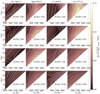 |
Fig. 9. Abundance correction differences obtained between the QM and our EFM models (in absolute values) for the lines Na I 5682 Å, Mg I 4702 Å, Al I 6696 Å and Si I 5772 Å as a function of Teff and log ɡ (represented by the shaded contour plots) and [Fe/H] (upper to lower panels). For comparison, the NLTE abundance corrections (also in absolute values) obtained by the QM models are represented by the iso-contour lines on the same plots using the same color scale. |
The abundances determined with the DRW, SH = 1.0 are similar to those obtained by the EFM and QM for different stellar parameters. The independence of the Si I NLTE corrections on the different H collisional models has also been shown in the previous studies of Bergemann et al. (2013) and Mashonkina et al. (2016a).
5. Removing the temperature dependence from the EFM
Finally, we test for the possible effects of removing the temperature dependencies of the EFM hydrogen collision rates from Eqs. (2) and (4), respectively. This is motivated by the fact that the fitting parameters depend weakly on temperature, as discussed in Sects. 2.1 and 2.2. Another motive is the possibility to decrease the number of fitting coefficients of the EFM from six for the CT and seven for the b−b rates, to four fitting parameters for each.
Applying the EFM to derive hydrogen collisional rates for atoms with no published quantum rates would require deriving these fitting parameters for the required atom by χ2 minimization fitting to spectra or measured EWs of benchmark or reference stars for a range of stellar parameters. This would require computing large grids of models for different combinations of fitting coefficients for each of the CT and b−b recipes in Eqs. (1) and (3). Decreasing the number of fitting parameters would typically simplify the process of deriving these coefficients. We therefore perform additional tests by computing NLTE abundances for the lines of each element using collision rates via the EFM with (i) constant temperature T = 4000 K for b−b rates, (ii) constant temperature T = 4000 K for both b−b and CT rates, (iii) constant temperature T = 6000 K for b−b rates, and finally (iv) constant temperature T = 6000 K for both b−b and CT rates. This was done again for the set of stellar parameters defined by our grid in Table 3.
We compared the NLTE abundance corrections computed with each of these four models for each element to those calculated with T-dependent EFM coefficients. The differences obtained from all the lines defined in Sect. 3 at all stellar parameters are represented by the box plots for each element in Fig. 10. The discrepancies between different T =constant models and the EFM are negligible for Na I lines, with differences of approximately zero (with a few outlier lines lying at < 0.004 dex). Using constant T = 6000 K collision rates for both b−b and CT collisions results in slightly larger but equally negligible differences up to −0.002 dex. For Mg I, the differences of most lines are within <0.005 dex for T = 4000 K and <0.01 for T = 6000 K, with a few outliers at <0.02 dex. For Al I, the constant T collisions lead to slightly larger corrections than the T-dependent EFM models to a maximum value of 0.02 dex, especially at T = 6000 K. A few outliers even deviate by up to −0.1dex from the EFM. Finally, for Si I lines, the corrections determined with the T-independent collisions differ slightly from the T-dependent ones within −0.005 dex at T = 4000 K and +0.01 dex at T = 6000 K.
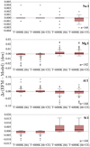 |
Fig. 10. Box plots representing the NLTE abundance correction differences obtained between models computed with T-dependent EFM rates and those computed with T-independent EFM rates for either the bb or both bb+CE collisions at T = 4000 K and T = 6000 K, respectively. The different panels show the results obtained at each model considered for each of the Na I, Mg I, Al I and Si I representative lines (Tables A.1– A.4) at all considered stellar parameters (Table 3). The number of lines, n, used by each model is also displayed on the plots. The solid black lines in the boxes show the median differences obtained at each model for each atom. Colored boxes represent 50%, and whisker edges (dotted black lines) 90% of the lines. Gray circles show the remaining outlier lines |
Overall, these results show that the NLTE calculations do not vary strongly by removing the T dependence from H collisional rates, except for a few outliers. This is especially the case upon using a constant T = 4000 K for both CT and b−b rates. The temperature dependencies can therefore be ignored in Eqs. (2.1) and (2.2). This allows the number of fitting coefficients of our proposed EFM model to be decreased to four for CT and for b−b rates, which can potentially be used to derive rate coefficients for elements for which no quantum rates yet exist. This is yet to be tested in future work.
6. Conclusions
We introduce an empirical fitting method (EFM) to estimate hydrogen collision rates to be used in NLTE abundance calculations. The method is based on fitting the published quantum rates of the neutral species for elements such as Be, Na, Mg, Al, Si and Ca with simple polynomial functions, whose rates show a very similar behavior as a function of transition energies. We provide two general fitting recipes, one for CT rates, and one for de-excitation rates, that can be used for all six elements. Sets of six and seven coefficients for b−b and CT collision processes, respectively, define the fits. The coefficients were found to vary slightly from one element to the next, but the variations remain within a range that suggest generality of the recipe. This implies that the recipes can potentially be used for elements with unknown hydrogen collision rates. The temperature dependence of the rates was taken into account, however, abundances were found to depend weakly on collision temperatures, which in principle can be removed from the fits. This decreases the number of fitting coefficients to four for each collisional process.
The fitting recipes were tested for their ability to reproduce the NLTE line profiles and abundance corrections of models incorporating quantum collisional rates (QM). These were determined for typical lines of four atoms for Na, Mg, Al and Si, over a grid covering a range of stellar parameters typical for FGK stars. For Na I lines, the NLTE corrections determined using the EFM are able to reproduce those computed with the QM rates to within ±0.03 dex for the warm dwarfs and subgiants, and to within 0.02 dex for the cool giants and dwarfs. For Mg I and Si I lines, while abundances for most lines lie within 0.05 dex of the QM abundances, larger differences were obtained for some cases up to 0.15 dex for Mg I, and 0.2 dex for Si I. This was especially the case for the subgiants and warm dwarfs. Smaller differences of <0.05 dex were obtained for the cool dwarfs and giants. The EFM performs well in reproducing the QM abundance corrections for the Al I lines. The majority of considered Al I lines lie within 0.03 dex of the reference QM models for different stellar atmospheric models. This is especially important for the metalpoor stars, where Al I NLTE abundance corrections can reach up to 0.6 dex at [Fe/H] = −3.0.
We also compared the abundance corrections obtained with the QM and EFM models to those calculated with the Drawin equation (DRW), incorporating the same excitation transitions as the QM, while ignoring ionization transitions by hydrogen. The absolute correction differences obtained between the QM and DRW models are larger in magnitude than those obtained between the QM and EFM models by up to 0.4 dex. This is especially the case for Na I, Mg I and Al I at lower metallicities. The discrepancies between the QM and DRW models at the optimal SH values for each species (0.1 for Na I, 1.0 for Mg I, 0.002 and 0.1 for Al I and 1.0 for Si I) are typically smallest for the solar metallicities. For the Si I lines, the corrections determined with the EFM are comparable to those computed with the DRW models for SH = 1.0. This agrees with previous studies for Si I (Bergemann et al. 2013; Mashonkina et al. 2016a) which showed that NLTE abundance corrections depend weakly on hydrogen collisions. Caution is advised, however, when comparing the abundance corrections derived by our DRW models to those determined in previous studies, as less H excitation and no ionization collisional transitions were incorporated in our models. This could potentially be driving the larger discrepancies obtained relative to the QM models, as compared to the literature.
Our proposed empirical fitting method, tested on four different neutral elements belonging to different groups from the period table, is able to reproduce the line profiles and NLTE abundance corrections of the same atoms incorporating ab-initio data, to within the abundance precisions described above for the different elements. It generally performs best for the cool and warm dwarfs, with slightly larger discrepancies obtained for the cool giants and subgiants. Future tests should exploit its ability to estimate the rates for energy levels that have not been included in the ab-initio calculations, and moreover, even potentially apply it to derive rates for other elements for which no quantum rates have yet been published.
Corresponding edits were made in the mul23_opacu.f routine in MULTI2.3.
Acknowledgments
We thank the anonymous referee for insightful comments and suggestions that have helped significantly to improve our paper. We thank Paul Barklem for valuable discussions on inelastic hydrogen collisions throughout the past years. Matthias Steffen is also thanked for making available his interpolation package. R.E. acknowledges support from a JINA-CEE fellowship, funded in part by the National Science Foundation under Grant No. PHY-1430152. T.M. and M.V.d.S.are supported by a grant from the Fondation ULB. This research was partially financed by the CEDRE PHC program, and the CNRS Programme National de Physique Stellaire. This work has made use of the VALD database, operated at Uppsala University, the Institute of Astronomy RAS in Moscow, and the University of Vienna and the Atomic Spectra Database hosted by the National Institute of Standards and Technology (NIST).
References
- Allen, C. W. 1973, Astrophysical quantities (London: University of London, Athlone Press) [Google Scholar]
- Allende Prieto, C., Majewski, S. R., Schiavon, R., et al. 2008, Astron. Nachr., 329, 1018 [Google Scholar]
- Andrievsky, S. M., Spite, M., Korotin, S. A., et al. 2007, A&A, 464, 1081 [NASA ADS] [CrossRef] [EDP Sciences] [Google Scholar]
- Andrievsky, S. M., Spite, M., Korotin, S. A., et al. 2008, A&A, 481, 481 [NASA ADS] [CrossRef] [EDP Sciences] [Google Scholar]
- Anstee, S. D., & O’Mara, B. J. 1995, MNRAS, 276, 859 [NASA ADS] [CrossRef] [Google Scholar]
- Asplund, M. 2005, ARA&A, 43, 481 [NASA ADS] [CrossRef] [Google Scholar]
- Barklem, P. S. 2016, Phys. Rev. A, 93, 042705 [NASA ADS] [CrossRef] [Google Scholar]
- Barklem, P. S. 2018, A&A, 612, A90 [NASA ADS] [CrossRef] [EDP Sciences] [Google Scholar]
- Barklem, P. S., & O’Mara, B. J. 1997, MNRAS, 290, 102 [Google Scholar]
- Barklem, P. S., Anstee, S. D., & O’Mara, B. J. 1998, PASA, 15, 336 [NASA ADS] [CrossRef] [Google Scholar]
- Barklem, P. S., Belyaev, A. K., Dickinson, A. S., & Gadéa, F. X. 2010, A&A, 519, A20 [NASA ADS] [CrossRef] [EDP Sciences] [Google Scholar]
- Barklem, P. S., Belyaev, A. K., Guitou, M., et al. 2011, A&A, 530, A94 [NASA ADS] [CrossRef] [EDP Sciences] [Google Scholar]
- Barklem, P. S., Anstee, S. D., & O’Mara, B. J. 2015, Astrophysics Source Code Library [record ascl:1507.007] [Google Scholar]
- Baumueller, D., & Gehren, T. 1996, A&A, 307, 961 [NASA ADS] [Google Scholar]
- Baumueller, D., & Gehren, T. 1997, A&A, 325, 1088 [NASA ADS] [Google Scholar]
- Belyaev, A. K. 2013, A&A, 560, A60 [NASA ADS] [CrossRef] [EDP Sciences] [Google Scholar]
- Belyaev, A. K., & Voronov, Y. V. 2017, A&A, 606, A106 [NASA ADS] [CrossRef] [EDP Sciences] [Google Scholar]
- Belyaev, A. K., & Yakovleva, S. A. 2017a, A&A, 608, A33 [NASA ADS] [CrossRef] [EDP Sciences] [Google Scholar]
- Belyaev, A. K., & Yakovleva, S. A. 2017b, A&A, 606, A147 [NASA ADS] [CrossRef] [EDP Sciences] [Google Scholar]
- Belyaev, A. K., Barklem, P. S., Spielfiedel, A., et al. 2012, Phys. Rev. A, 85, 032704 [NASA ADS] [CrossRef] [Google Scholar]
- Belyaev, A. K., Yakovleva, S. A., & Barklem, P. S. 2014, A&A, 572, A103 [NASA ADS] [CrossRef] [EDP Sciences] [Google Scholar]
- Belyaev, A. K., Voronov, Y. V., Yakovleva, S. A., et al. 2017, ApJ, 851, 59 [NASA ADS] [CrossRef] [Google Scholar]
- Bergemann, M., Kudritzki, R.-P., Würl, M., et al. 2013, ApJ, 764, 115 [NASA ADS] [CrossRef] [Google Scholar]
- Bergemann, M., Collet, R., Amarsi, A. M., et al. 2017, ApJ, 847, 15 [NASA ADS] [CrossRef] [Google Scholar]
- Carlsson, M. 1986, Uppsala Astronomical Observatory Reports, 33 [Google Scholar]
- Carlsson, M. 1992, in Cool Stars, Stellar Systems, and the Sun, eds. M. S. Giampapa, & J. A. Bookbinder, ASP Conf. Ser., 26, 499 [NASA ADS] [Google Scholar]
- Castelli, F., & Kurucz, R. L. 2010, A&A, 520, A57 [NASA ADS] [CrossRef] [EDP Sciences] [Google Scholar]
- Drawin, H.-W. 1968, Z. Angew. Phys., 211, 404 [Google Scholar]
- Drawin, H. W. 1969a, Z. Angew. Phys., 225, 470 [Google Scholar]
- Drawin, H. W. 1969b, Z. Angew. Phys., 225, 483 [Google Scholar]
- Ezzeddine, R., Merle, T., & Plez, B. 2016, Astron. Nachr., 337, 850 [NASA ADS] [CrossRef] [Google Scholar]
- Gehren, T., Liang, Y. C., Shi, J. R., Zhang, H. W., & Zhao, G. 2004, A&A, 413, 1045 [NASA ADS] [CrossRef] [EDP Sciences] [Google Scholar]
- Gilmore, G., Randich, S., Asplund, M., et al. 2012, The Messenger, 147, 25 [NASA ADS] [Google Scholar]
- Guitou, M., Spielfiedel, A., Rodionov, D. S., et al. 2015, Chem. Phys., 462, 94 [NASA ADS] [CrossRef] [Google Scholar]
- Gustafsson, B., Edvardsson, B., Eriksson, K., et al. 2008, A&A, 486, 951 [NASA ADS] [CrossRef] [EDP Sciences] [Google Scholar]
- Heiter, U., Jofré, P., Gustafsson, B., et al. 2015, A&A, 582, A49 [NASA ADS] [CrossRef] [EDP Sciences] [PubMed] [Google Scholar]
- Lambert, D. L. 1993, Phys. Scr. Volume T, 47, 186 [NASA ADS] [CrossRef] [Google Scholar]
- Lind, K., Asplund, M., Barklem, P. S., & Belyaev, A. K. 2011, A&A, 528, A103 [Google Scholar]
- Mashonkina, L. 2013, A&A, 550, A28 [NASA ADS] [CrossRef] [EDP Sciences] [Google Scholar]
- Mashonkina, L. I., Shimanski˘ı, V. V., & Sakhibullin, N. A. 2000, Astron. Rep., 44, 790 [NASA ADS] [CrossRef] [Google Scholar]
- Mashonkina, L. I., Belyaev, A. K., & Shi, J.-R. 2016a, Astron. Lett., 42, 366 [NASA ADS] [CrossRef] [Google Scholar]
- Mashonkina, L. I., Sitnova, T. N., & Pakhomov, Y. V. 2016b, Astron. Lett., 42, 606 [NASA ADS] [CrossRef] [Google Scholar]
- Merle, T., Thévenin, F., Pichon, B., & Bigot, L. 2011, MNRAS, 418, 863 [NASA ADS] [CrossRef] [Google Scholar]
- Merle, T., Thévenin, F., & Zatsarinny, O. 2015, A&A, 577, A113 [NASA ADS] [CrossRef] [EDP Sciences] [Google Scholar]
- Mitrushchenkov, A., Guitou, M., Belyaev, A. K., et al. 2017, J. Chem. Phys., 146, 014304 [NASA ADS] [CrossRef] [Google Scholar]
- Nordlander, T., Amarsi, A. M., Lind, K., et al. 2017, A&A, 597, A6 [NASA ADS] [CrossRef] [EDP Sciences] [Google Scholar]
- Osorio, Y., Barklem, P. S., Lind, K., et al. 2015, A&A, 579, A53 [NASA ADS] [CrossRef] [EDP Sciences] [Google Scholar]
- Peterson, R. C., & Kurucz, R. L. 2015, ApJS, 216, 1 [Google Scholar]
- Saha, M. N. 1921, Proc. R. Soc. London, Ser. A, 99, 135 [NASA ADS] [CrossRef] [Google Scholar]
- Seaton, M. J. 1962a, Proc. Phys. Soc., 79, 1105 [NASA ADS] [CrossRef] [Google Scholar]
- Seaton, M. J. 1962b, in Atomic and Molecular Processes, ed. D. R. Bates, 375 [Google Scholar]
- Shi, J. R., Gehren, T., Butler, K., Mashonkina, L. I., & Zhao, G. 2008, A&A, 486, 303 [NASA ADS] [CrossRef] [EDP Sciences] [Google Scholar]
- Steenbock, W., & Holweger, H. 1984, A&A, 130, 319 [NASA ADS] [Google Scholar]
- Steenbock, W., & Holweger, H. 1992, Lect. Notes Phys., 401, 57 [NASA ADS] [CrossRef] [Google Scholar]
- Steffen, M. 1990, A&A, 239, 443 [NASA ADS] [Google Scholar]
- Steinmetz, M., Zwitter, T., Siebert, A., et al. 2006, AJ, 132, 1645 [NASA ADS] [CrossRef] [Google Scholar]
- Thévenin, F., & Idiart, T. P. 1999, ApJ, 521, 753 [NASA ADS] [CrossRef] [Google Scholar]
- Thomson, J. J. 1912, Philos. Mag., 23, 499 [Google Scholar]
- Travis, L. D., & Matsushima, S. 1968, ApJ, 154, 689 [NASA ADS] [CrossRef] [Google Scholar]
- Unsold, A. 1955, Physik der Sternatmospharen, MIT besonderer Berucksichtigung der Sonne (Berlin: Springer) [Google Scholar]
- van Regemorter, H. 1962, ApJ, 136, 906 [NASA ADS] [CrossRef] [Google Scholar]
- Yakovleva, S. A., Voronov, Y. V., & Belyaev, A. K. 2016, A&A, 593, A27 [NASA ADS] [CrossRef] [EDP Sciences] [Google Scholar]
- Yakovleva, S. A., Barklem, P. S., & Belyaev, A. K. 2018, MNRAS, 473, 3810 [NASA ADS] [CrossRef] [Google Scholar]
- Zatsarinny, O., Bartschat, K., & Gedeon, S. 2009, J. Phys. Conf. Ser., 194, 042029 [NASA ADS] [CrossRef] [Google Scholar]
Appendix A: Line data - NLTE corrections
Tables A.1–A.4, listing the NLTE corrections obtained for selected lines of Na I, Mg I, Al I and Si I are only available at the CDS. The corrections are computed with four different atoms for each element of different implementations of hydrogen collisions using (i) the published quantum rates (QM), (ii) our proposed fitting method (EFM), (iii) the Drawin equation with SH = 0.1 (DRW, SH = 0.1) (iv) the Drawin equation with SH = 1.0 (DRW, SH = 1.0), as well as (v) the Drawin equation with SH = 0.002 (DRW, SH = 0.002) for Al I, for a range of stellar parameters defined in Table 3.
All Tables
CT and b−b hydrogen collision rate fitting coefficients obtained for the neutral species of Be, Na, Mg, Al, Si and Ca.
Atomic databases and references used for the sources of energy levels and radiative and collisional b−b and b−f transitions used for each species in our model atoms for Na, Mg, Al and Si.
Grid of stellar parameters for which the NLTE calculations for all atoms were performed.
All Figures
|
Fig. 1. CT rate coefficients (in logarithmic scale), log QCT, as a function of inverse transition energies |
| In the text | |
|
Fig. 2. CT rate coefficients log QCT at T = 6000 K, for Be I, Na I, Mg I, Al I, Si I and Ca I (filled triangles) from the quantum calculations of Yakovleva et al. (2016), Barklem et al. (2010), Belyaev et al. (2012, 2014, 2017), Guitou et al. (2015), Belyaev (2013), respectively. The polynomial fits as per the EFM (dashed red lines) are also displayed on the plots. |
| In the text | |
|
Fig. 3. Temperature dependence plots for the CT rate fitting coefficients a1, a2, |
| In the text | |
|
Fig. 4. De-excitation rate coefficients log Qb−b at T = 6000 K (in logarithmic scale) for Be I, Na I, Mg I, Al I, Si I and Ca I from the quantum calculations of Yakovleva et al. (2016), Barklem et al. (2010), Belyaev et al. (2012, 2014, 2017), Guitou et al. (2015), Belyaev (2013), respectively. Their corresponding polynomial fits (dashed red lines) are also shown. |
| In the text | |
|
Fig. 5. Line profiles of Na I 6154 Å, Mg I 4730 Å, Al I 6696 Å and Si I 5772 Å computed using different hydrogen collision models: QM (black lines), EFM (red lines), DRW, SH = 0.1 (blue lines), DRW, SH = 0.1 (olive lines) and DRW, SH = 0.002 for Al I (magenta lines). The lines were computed at Teff = 4500, log ɡ = 2.5 and for two metallicities, [Fe/H] = +0.00 (left panels) and [Fe/H] = −3.00 (right panels). The χ2 differences obtained between each model relative to the QM are shown on the plots. |
| In the text | |
|
Fig. 6. Box plots showing the overall NLTE abundance correction differences obtained between models computed with the QM rates and those computed with the EFM, DRW, SH = 0.1 and DRW, SH = 1.0 rates (for Al I, we choose to show results for DRW, SH = 0.002 instead of DRW, SH = 1.0). Boxes in each panel display the differences obtained from representative lines of Na I, Mg I, Al I and Si I (shown in Table A.1) for the corresponding stellar parameters of cool dwarfs (in red), cool giants (in green), subgiants (in blue) and warm dwarfs (in magenta) in the left-hand panels. Right-hand panels show the same plots for different metallicities. The number of lines, n, used in each box plot is displayed. Black solid lines show the median values obtained for each model and each atom, colored boxes represent 50%, and whisker edges 90% of the lines. Gray circles show the remaining outlier lines. |
| In the text | |
|
Fig. 7. Abundance correction differences obtained between the QM and the corresponding EFM (empty circles), DRW, SH = 0.1 (empty squares) and DRW, SH = 0.1 collision models (empty triangles), as well as DRW, SH = 0.002 for Al I, (empty stars) for select Na I, Mg I, Al I and Si I lines, as a function of [Fe/H]. This is shown for the cool giants and dwarfs (left-hand and middle panels), as well as the warm dwarfs (right-hand panels) stellar parameters. The NLTE abundance corrections obtained by the QM models are also shown (filled diamonds), for comparison. |
| In the text | |
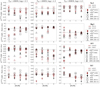 |
Fig. 8. As in Fig. 7 but showing different lines for Na I, Mg I, Al I and Si I. |
| In the text | |
|
Fig. 9. Abundance correction differences obtained between the QM and our EFM models (in absolute values) for the lines Na I 5682 Å, Mg I 4702 Å, Al I 6696 Å and Si I 5772 Å as a function of Teff and log ɡ (represented by the shaded contour plots) and [Fe/H] (upper to lower panels). For comparison, the NLTE abundance corrections (also in absolute values) obtained by the QM models are represented by the iso-contour lines on the same plots using the same color scale. |
| In the text | |
|
Fig. 10. Box plots representing the NLTE abundance correction differences obtained between models computed with T-dependent EFM rates and those computed with T-independent EFM rates for either the bb or both bb+CE collisions at T = 4000 K and T = 6000 K, respectively. The different panels show the results obtained at each model considered for each of the Na I, Mg I, Al I and Si I representative lines (Tables A.1– A.4) at all considered stellar parameters (Table 3). The number of lines, n, used by each model is also displayed on the plots. The solid black lines in the boxes show the median differences obtained at each model for each atom. Colored boxes represent 50%, and whisker edges (dotted black lines) 90% of the lines. Gray circles show the remaining outlier lines |
| In the text | |
Current usage metrics show cumulative count of Article Views (full-text article views including HTML views, PDF and ePub downloads, according to the available data) and Abstracts Views on Vision4Press platform.
Data correspond to usage on the plateform after 2015. The current usage metrics is available 48-96 hours after online publication and is updated daily on week days.
Initial download of the metrics may take a while.