| Issue |
A&A
Volume 617, September 2018
|
|
|---|---|---|
| Article Number | A90 | |
| Number of page(s) | 10 | |
| Section | Cosmology (including clusters of galaxies) | |
| DOI | https://doi.org/10.1051/0004-6361/201833471 | |
| Published online | 21 September 2018 | |
Fingerprint of Galactic Loop I on polarized microwave foregrounds
1
The Niels Bohr Institute & Discovery Center, Blegdamsvej 17, 2100
Copenhagen, Denmark
2
Key laboratory of Particle and Astrophysics, Institute of High Energy Physics, CAS, 19B YuQuan Road, Beijing, PR China
e-mail: This email address is being protected from spambots. You need JavaScript enabled to view it.
Received:
22
May
2018
Accepted:
15
June
2018
Abstract
Context. Currently, detection of the primordial gravitational waves using the B-mode of cosmic microwave background (CMB) is primarily limited by our knowledge of the polarized microwave foreground emissions. Improvements of the foreground analysis are therefore necessary. As we revealed in an earlier paper, the E-mode and B-mode of the polarized foreground have noticeably different properties, both in morphology and frequency spectrum, suggesting that they arise from different physicalprocesses, and need to be studied separately.
Aims. I study the polarized emission from Galactic loops, especially Loop I, and mainly focus on the following questions: Does the polarized loop emission contribute predominantly to the E-mode or B-mode? In which frequency bands and in which sky regions can the polarized loop emission be identified?
Methods. Based on a well known result concerning the magnetic field alignment in supernova explosions, a theoretical expectation is established that the loop polarizations should be predominantly E-mode. In particular, the expected polarization angles of Loop I are compared with those from the real microwave band data of WMAP and Planck.
Results and conclusions. The comparison between model and data shows remarkable consistency between the data and our expectations at all bands and for a large area of the sky. This result suggests that the polarized emission of Galactic Loop I is a major polarized component in all microwave bands from 23 to 353 GHz, and a considerable part of the polarized foreground likely originates from a local bubble associated with Loop I, instead of the far more distant Galactic emission. This result also provides a possible way to explain the E-to-B excess problem by contribution of the loops. Finally, this work may also provide the first geometrical evidence that the Earth was hit by a supernova explosion.
Key words: cosmic background radiation / cosmology: observations / methods: data analysis / ISM: bubbles / ISM: magnetic fields
© ESO 2018
1. Introduction
Galactic Loop I is a large circular structure on the north Galactic sky whose brightest part is also referred to as the north polar spur (NPS) (Berkhuijsen et al. 1971; Salter 1983). It shines from the radio band to the γ-ray band Haslam et al. (1981a,b), including microwaves (Bennett et al. 2013; Planck Collaboration I 2016), and possibly even affects the cosmic rays (Bhat et al. 1985). The origin of this structure is suggested to be an old supernova (Berkhuijsen et al. 1971; Salter 1983; Wolleben 2007) that created its own local bubble which happens to be in close contact with the Orion local bubble (Egger & Aschenbach 1995; Breitschwerdt & de Avillez 2006). The brightest part of Loop I is a few tens of degrees in width, and is about 60° away from its center, whose sky direction is around (l, b) = (329°, 17.5°) (Berkhuijsen et al. 1971; Mertsch & Sarkar 2013). The distance of the old supernova is not well determined, but could be of the order of 102 pc (Mertsch & Sarkar 2013). Estimating from its roughly 60° angular radius, the wavefront of the explosion must have already traveled at least half the distance between its point of origin and Earth.
Although it is quite natural to imagine that the Earth could have been hit by a supernova explosion, to date, there is only indirect evidence provided by statistical expectation (Whitten et al. 1976; Clark et al. 1977); oceanic traces of 60Fe (Knie et al. 2004), 44Ti (Fields & Ellis 1999; Burgess & Zuber 2000), and other isotopes (Fields et al. 2005); and a combined estimation (Benítez et al. 2002). In principle, much more direct evidence could be obtained by geometric considerations: before the explosion hits the Earth, observers facing the supernova can only see its signal from the front side. Therefore, if one sees the supernova signal from both front and back sides, then the Earth must have been hit by the supernova explosion. The most difficult part of this idea is how to associate a signal coming from the back side with a supernova remnant lying in the front side. Fortunately, in this work it is shown that this problem can be solved by comparing the polarization angles measured in the microwave bands with the assumption of a minimal Loop I model.
As briefly introduced in Appendix A, the polarized signals can be decomposed into the E and B modes. It was suggested by Liu et al. (2018) that for a better foreground removal, such EB decomposition should be done in form of (1)
(1)
If the (Q E, U E) and (Q B, U B) signals are found to be associated with different physical mechanisms, then such decomposition is a natural choice. This is confirmed in this work by showing that the loop polarizations are predominantly E-mode.
The paper is organized as follows: Sect. 2 explains why the loop polarizations are predominantly E-mode, which is also observable in real data. Section 3 proposes a simplified model for the Loop I polarization angles that contains no free parameters, and which is found to be consistent with the real foregrounds at 99.999% confidence level. This strongly supports that the polarized microwave foregrounds are largely from Loop I, as well as that the Earth has been hit by the Loop I supernova explosion. Finally, the results are discussed in Sect. 4 and conclusions are given in Sect. 5.
2. Loops and E-mode
2.1. Why the loops are predominantly E-mode
This work starts from a simple model of the loop polarizations, which allows several trivial parameters (position, size, radial profile, intensity, etc.) but there is only one major assumption: signals from the loop are polarized along the radial directions of the supernova. This assumption is based on the conclusion that the shell magnetic fields are along the tangent directions (van der Laan 1962), which was confirmed by Whiteoak & Gardner (1968) and Milne (1987), and recently reviewed and developed by Dubner & Giacani (2015) and Petruk et al. (2016). We also note that this major assumption is not a new one: application and verification of this assumption on the microwave maps can also be found in Vidal et al. (2015), for example.
More discussions supporting this major assumption can be found in Appendix B, but the assumption itself is pure geometry and is easy to apply. A typical model for Loop I polarization is therefore generated, as follows: First I take a Gaussian radial profile for the polarization intensity, which is maximized and equal to 1 at 58° to the center of Loop I (58° is the angular radius of the brightest part of Loop I), and with a 20° FWHM (the FWHM parameter will affect the shape of the angular power spectrum, but here we mainly pay attention to “zero or not”, and therefore this parameter is not important). Then the polarization angles are set to along the radial directions of Loop I. The result of this model is shown in Fig. 1 and compared with the real Loop I polarization angles at the WMAP K-band (22.8 GHz) with a 20° wide mask to emphasis the NPS region. However, we note that the model is actually full sky, with the main power being localized around Loop I. This is very convenient in avoiding the leakage from E-mode to B-mode, because such leakage does not exist for a full sky map. The full sky angular power spectra of the model is calculated and shown in the lower panel of Fig. 1.
 |
Fig. 1. Upper left: example of the expected loop polarization directions (by small black lines). Upper right: polarization directions of the WMAP K-band in the Loop I region, with Loop I marked by a black circle. The color scales of the upper panels are for the polarized intensity, which is 0 ~100 μK for the K-band and −1 ~ 1.2 for the model (here the absolute amplitude of polarization intensity is meaningless for the model, and therefore such an unphysical range is chosen to maximize the visibility of the thin lines). Lower: the angular power spectrum of the model shown in upper-left, calculated without a mask. We note that the polarization directions in the model are strictly along the normal vectors, and some small misalignments are only visual effects due to pixelization. |
The excellent agreement between the polarization angles of the model and data shown in the upper panels of Fig. 1 fully supports the above major assumption. Subsequently, by connecting Fig. 1 with the geometrical interpretation of the E and B modes in real space (see Appendix A), one can see that this major assumption can produce only E-mode polarizations. This is confirmed by the angular power spectra of the model in Fig. 1, which is calculated as described above. The angular power spectra have positive EE & TE spectra, but these are zero for BB & TB. We note that this important property depends only on the major assumption1.
Therefore, polarized loop signals will form an E-mode foreground family, whose presence will certainly provide net EE and TE excess. This can be naturally associated with the E-mode excess reported by Planck Collaboration Int. XXX (2016) in terms of an E-to-B ratio roughly equal to 2. This is discussed in Sect. 2.3.
2.2. E-mode loops/arches in real data
To directly investigate the E-mode loops in real data, the WMAP K-band and Planck 353 GHz full sky polarization maps are decomposed using Eq. (1), and the E and B mode polarization intensities calculated as  and
and  , respectively. The results of such decomposition are shown in Fig. 2. Apparently, after decomposition, all loop structures2 are visible in P
E but disappear in P
B, which strongly supports the conclusion that loop polarizations are an E-mode foreground family. This was also tested by Liu et al. (2018).
, respectively. The results of such decomposition are shown in Fig. 2. Apparently, after decomposition, all loop structures2 are visible in P
E but disappear in P
B, which strongly supports the conclusion that loop polarizations are an E-mode foreground family. This was also tested by Liu et al. (2018).
 |
Fig. 2. Polarization intensity maps and their EB decompositions at the K-band (upper) and 353 GHz (lower). From left to right: total polarized intensity P, P E, and P B. The loop-like structures are marked by black or white lines depending on visibility. They are apparently visible in E-mode (middle) but disappear in B-mode (right). |
The ratio between the E and B mode polarization intensities is calculated as ρ = P E/P B and presented in Fig. 3, especially for the arch regions. The median and mean values of ρ = P E/P B are compared for inside and outside the arch regions, and the results are listed in Table 1. For all cases, ρ are apparently higher for the inside regions, which further supports the argument that loop polarizations are mainly E-mode. A simple test is then done to show the significance of the values in Table 1: for each band, the corresponding arch mask is rotated to 192 evenly distributed directions (corresponding to N side = 4), and for each direction, the new mean value is calculated inside the new mask. For the K-band, none of the 192 new directions give a higher mean value of ρ than the unrotated one (5.4), therefore the confidence level is at least 99.5%. Similarly, for 353 GHz the confidence level is 99%.
 |
Fig. 3. Ratio ρ = P E/P B in K-band (upper) and 353 GHz (lower), both full sky and around the same arches as marked in Fig. 2. The outline of the BICEP2 zone is marked in thick dash line. |
2.3. Loops and E-mode excess
It was reported by the Planck Collaboration Int. XXX (2016) that there is an excess of the E-mode foreground in the 353 GHz band with an EE-to-BB ratio of approximately two, and possible explanations were proposed based on the MHD properties; see, for example, Caldwell et al. (2017), Kandel et al. (2017) and Kritsuk et al. (2018). With the proposals from Sect.s 2.1–2.2, a parallel direction is opened, in which the E-mode excess can be naturally explained by the existence of the loops. Detailed works in this direction will follow, and a tentative estimation is that, due to the reported E-to-B ratio, the loops can contribute as much as the ordinary diffuse Galactic foreground emission, which is expected to have similar E and B mode spectra.
We also note that, for the loop polarizations, the shape of their E-mode angular power spectra is determined by the choice of the trivial parameters. Since the real sky can possibly contain many loop-like structures (Kiss et al. 2004; Könyves et al. 2007; Mertsch & Sarkar 2013; Vidal et al. 2015), it is quite possible to fit the observed polarized foreground spectrum by a family of loops, which is an interesting direction for future work.
3. Model without free parameters
An important adjustment of the basic model discussed in Sect. 2.1 is to eliminate all free parameters and fix the model. This has the great advantage that no fitting is needed at all, and the model is therefore completely independent from the data.
This is done as follows:
-
Only the polarization angles are considered, so all parameters about amplitude become irrelevant.
-
The Loop I emission is regarded as coming from the associated bubble3 whose radius can be bigger than the distance to its center, such that the emission can cover the full sky.
-
Finally, with the major assumption mentioned at the beginning of Sect. 2.1 and the already known (l, b) coordinates of the Loop I central supernova remnant, all polarization angles can be calculated without any other parameters or assumptions.
Following the above procedures, one obtains a full sky pattern of the Loop I polarization angles. We note that, although the emissions from Loop I were not regarded as covering the full sky before, people have already discussed the possibility that the signal from Loop I is extended beyond the NPS region; for example, Planck Collaboration XXV (2016) and Vidal et al. (2015).
3.1. Visual inspection
A completely determined model means no need for fitting, and therefore the full sky polarization angles can be calculated straightforwardly and compared with the polarization angles measured at the WMAP K-band (2° smoothing), as shown in Fig. 4. By simple visual inspection, one can easily see qualitative similarity between the model and data for the greater part of the sky: In the north sky, starting from the central black line, the color on the left-hand side starts from green and goes anti-clockwise along the color disc4 until green again; while in the right hand side (still north) the color starts from yellow and goes clockwise to green. Similarly, in the south sky the color variation left of the central black line is clockwise from purple to blue, and for the right-hand side it is anticlockwise from purple to blue. All these color rotations are the same for both the data and the Loop I model, which indicates that the polarized microwave emission is associated with Loop I for a large area of the sky.
 |
Fig. 4. Left: polarization angles calculated from the minimal model, with no free parameters and no fitting. Middle: the real data (WMAP K-band). Right: real data and only E-mode. The color-to-angle mapping is given by the low-left color disk,and the black circle is the critical range that is 90° from the center of Loop I. |
We note that the model-to-data comparison can be made more fair by considering only the E-mode of the WMAP K-band data. Doing so, one does see better data-to-model consistency, which is expected, especially in the lower-right corner of the map, as also presented in Fig. 4.
3.2. Significance estimation
The visual inspection in Sect. 3.1 is good for understanding, but is not quantitative. For example, the red and yellow colors are visually very different, but the corresponding angles can be close to each other. Therefore, the consistency between data and model is quantitatively tested below using the mean angle difference (MAD) 〈δθ 〉 defined below.
Allowing the polarization angle difference to be  , by the definition of polarization angles,
  is identical to
  . Moreover, if one disregards the sign, then
  is also identical to
  . To reflect these symmetries, in this work, the polarization angle difference is defined as
 (2)
(2)
where δθ
always lies in the range 0°–90°, and all four angles  and
and  are regarded as equivalent. Subsequently, the MAD 〈δ
θ
〉 is defined as
are regarded as equivalent. Subsequently, the MAD 〈δ
θ
〉 is defined as (3)
(3)
where the arctan2 function is a variant of the arctan function that takes two parameters to return a result in the range [0, 2π]. With the above definition, the similarity between two sets of angles can be roughly evaluated by cos(〈δ θ 〉), where cos(〈δ θ 〉) = 1 indicates that the two sets of angles are identical. For two independent maps, the expectation of 〈δ θ 〉 should be centered around 45°, and due to the central limit theorem, for data sets with more degrees of freedom (such as more pixels), the distribution of 〈δ θ 〉 is more narrow and Gaussian.
The sky region at low Galactic latitudes is dominated by the strong emission from the Galactic plane, and therefore a ring mask is used to exclude |b| ≤ 20°. Meanwhile, the area with very low polarized signal is dominated by noise, which is uncorrelated with any real signal, and therefore a fraction ρ = 25% of the sky5 with the lowest P E is also excluded. The loop signal is expected to decay with increasing radius to the center, and so only the region less than 120° from the center of Loop I is used. The combined mask is shown in the left panel of Fig. 5.
 |
Fig. 5. Regions used to estimate the significance of the model-to-data association, where red means usable region and green means masked region. Left: the region used in Sect. 3.2. Middle and right: the inside and outside regions used in Sect. 3.3, which are 0°–90° and 90°–120° to the center of Loop I, respectively. The BICEP2 region is also marked in each panel. |
The MAD between the real K-band map and the minimal model is first calculated with the mask shown in the left panel of Fig. 5, which is 〈δ
θ
〉 = 15.6°, with cos(〈δ
θ
〉) = 0.96, very close to 1. Realistic simulations are then run: First the input (Q, U) Stokes parameter map is converted into  using HEALPix (Górski et al. 2005). Subsequently, the phases for
  and
and  are randomized before inverse transforming to real space using HEALPix to get a simulated map. Since the EE and BB spectra are unaffected by the phases, such an operation completely changes the morphology of the input map without changing its E and B spectra. We note that the B-mode is set to zero in the simulations because the model is also pure E-mode. Using 105 simulations generated like this, I find none that yield a MAD below 20° for the region in use, as illustrated by the histograms of all simulations in Fig. 6. According to this test, the E-mode of the K-band foreground map gives polarization angles that are consistent with those calculated in our minimal model at a 99.999% confidence level6.
 |
Fig. 6. Histograms of 105 mean angle differences 〈δ θ 〉 between the minimal model and simulations, on which results from the real data are marked by thin vertical lines, and the 45° expectation of 〈δ θ 〉 is marked by the central vertical line. |
3.3. Critical range and the BICEP2 region
Now I discuss how to determine whether the supernova has hit the Earth or not. The division between the front and back sides is made at 90° from the loop center, which is marked by a black circle in Fig. 4. If the similarity between the minimal model and the data is significant for both sides of the black circle, then it is suggested that the Earth has been hit by the Loop I supernova explosion.
For this purpose, the region shown in the left panel of Fig. 5 is divided into two sub-regions and shown in the same figure as the middle and right panels: the middle panel shows the inside region (front side, from 0° to 90°), and the right panel shows the outside region (back side, from 90° to 120°). The resulting MAD for the inside region is 〈δ θ 〉 = 16.2°, with cos(〈δ θ 〉) = 0.96; and for the outside region is 〈δ θ 〉 = 14.3°, with cos(〈δ θ 〉) = 0.97. Using 105 simulations generated as described in Sect. 3.2 for the two regions respectively, I find the values of both regions to be significant at a 99.999% confidence level, which are also shown in Fig. 6 by red and blue lines. Therefore, both the inside and outside regions are suggested to be associated with Loop I, which means we are likely sitting inside the bubble of Loop I.
Meanwhile, the above calculation is also done for the BICEP2 region shown in Fig. 5 and the result is included in Fig. 6, which has an exceptionally low value of 〈δ θ 〉 = 9.7° and cos(〈δ θ 〉) = 0.99. Due to the smaller size of the BICEP2 region, the distribution of 〈δ θ 〉 is much wider and is apparently non-Gaussian. Using 105 simulations, I find the association between Loop I and the BICEP2 region is still confirmed at 99.96%.
3.4. Other frequencies and CMB
The analyses presented in Sects. 3.2 and 3.3 are also done for all the WMAP and Planck frequency bands that contain polarization data, including the WMAP K, Ka, Q, V, W; and the Planck 30, 44, 70, 100, 143, 217, 353 GHz. The Planck SMICA CMB map with polarization is subtracted from each of them to roughly remove the CMB7, and the Planck LFI bandpass mismatch correction is applied to 30, 44, and 70 GHz bands. A complete list of 〈δ θ 〉 is presented as Table 2, in which one can see that all of them give apparently lower 〈δ θ 〉 than the 45° expectation, where the minimal confidence level is no less than 99% for each band. This means all WMAP and Planck frequency bands are significantly contaminated by the Loop I polarized emissions. If all bands are regarded as independent, then the combination of them gives a surprisingly high confidence level.
List of 〈δ θ 〉 in degrees between the minimal Loop I model and 23–353 GHz bands.
I also note that the Planck 30 and 44 GHz bands (marked in blue in the table) give apparently higher 〈δ θ 〉 than their neighbors, especially the 30 GHz band. This is most likely due to the bandpass mismatch leakage (Planck Collaboration II 2016; Planck Collaboration III 2016) that remains even after correction (Weiland et al. 2018). A similar abrupt 〈δ θ 〉 value exists for the Planck 100 GHz band in the BICEP2 region, which is also marked in blue. On the other hand, the case for the Planck 70 GHz band is slightly unclear: it is also contaminated by the bandpass mismatch leakage, but the amplitude of contamination is regarded as less than 30 and 44 GHz. One can still see from Table 2 that 70 GHz has moderately higher 〈δ θ 〉 than its neighbors, which could be due to either the remaining bandpass mismatch leakage, or relatively lower polarized foreground at 70 GHz. The latter could be good news for detection of the primordial B-mode; however, since a full consideration of the systematics is very complicated, the above discussions are only suggestive. An updated study will be possible when the future Planck data release becomes available, which may come with lower systematic errors.
The value of 〈δ θ 〉 is also calculated between the minimal model and the Planck SMICA CMB map. In this case, for the three masks shown in Fig. 5, 〈δ θ 〉 are 41.4°, 43.1° and 38.5°, respectively. Interestingly, these values are much closer to 45°, but are still systematically lower, which indicates a possible residual loop contamination even in the final CMB polarization product.
4. Discussion
It was pointed out by Liu et al. (2014) and von Hausegger et al. (2016) that the Galactic Loop I may leave a trace on the final CMB intensity map, which is partly verified in this work for the E-mode. This provides a good reason to follow the suggestions by Liu et al. (2018) to adopt the decomposition in Eq. (1), which may help to improve the estimation of the CMB B-mode.
For an incomplete sky coverage (which is the case for all individual ground missions), the above decomposition is inevitably affected by the E-to-B and B-to-E leakage. Although there are already many methods to prevent such leakages (Smith 2006; Kim & Naselsky 2010; Zhao & Baskaran 2010; Bunn & Wandelt 2017; Kodi Ramanah et al. 2018), they are mainly designed for Gaussian and homogeneous CMB signals, and are therefore problematic for non-Gaussian, inhomogeneous signals such as diffuse Galactic foregrounds. Therefore, a large (or even full) sky coverage – either by combining various ground missions or from a space mission (Hazumi et al. 2012; Challinor et al. 2018) – is apparently preferred for detection of primordial gravitational waves.
If the supernova explosion is spherically symmetric, then by our major assumption, the loop emission is 100% E-mode. However, in reality, the supernova explosion could be asymmetric, and therefore there could be residual B-mode emission from the loops. For example, a multiple supernova explosion scenario was studied by Vasiliev et al. (2017), in which the overall shape of the shell is naturally asymmetric. Also, in Fig. 2, although much fainter, one can still see some suspicious loop-like structures in the P B map, which might be this kind of residual. Meanwhile, another source of the B-mode from loops due to projection is also discussed in Appendix B.
Recent work (Liu et al. 2018) has confirmed that for both the E-mode and the B-mode families in the BICEP2 zone, the polarization angles are almost the same from 217 to 353 GHz; meanwhile, Table 2 tells us that in the BICEP2 zone, the polarization angle is tightly related to Loop I. These two facts highlight the possibility that the B-component from Loop I (if any) may also affect the high Galactic latitudes, such as the BICEP2 area.
It should also be noted that the LSA model (Page et al. 2007) for the Galactic magnetic field can also give results that are consistent with the WMAP K-band polarization angles, and can explain the typical foreground polarization fraction. The disadvantage of this model is that it requires the fitting of several free parameters regarding the Galactic spiral structure and the highenergy electron distribution, whereas the model in Sect. 3 has no free parameters and requires no fitting, making it the preferable option. Moreover, to avoid circular argument, a model based on fitting can only provide indications of the general trends of the data, and cannot be used for further purposes, such as explaining the E-mode excess – which can be done easily and naturally using a study such as the one presented here. In reality, however, the line-of-sight integration for the polarized signal consists of both local and remote parts, and therefore reality is more likely to be better represented by a combination of this work and the LSA model.
The polarized signal can change its polarization direction due to integration along the line-of-sight (LOS), and such integration can easily decrease the total polarization intensity, which is called depolarization. Such depolarization is considered both by Page et al. (2007) and in Appendix B, as well as in studies of three-dimensional foreground analysis (Sun et al. 2008; Fauvet et al. 2011; Green et al. 2015; Martínez-Solaeche et al. 2017). All these works depend on our knowledge of the Galactic and local magnetic field, which remains far from perfect. Therefore, a three-dimensional analysis for polarized foreground still requires better constraints.
5. Conclusion
The main conclusions of this work are listed below:
-
The supernova explosions can produce predominantly E-mode foreground (Sect. 2.1).
-
The E-mode loops provide a new way to explain the E-to-B excess phenomenon (Sect. 2.3).
-
A large part of the polarized foreground is likely coming from a local bubble associated with Loop I, which suggests that the Earth was hit by a supernova explosion (Sect. 3.3).
-
The E-mode foreground from Loop I is identified at all WMAP and Planck frequency bands and for a large area of the sky, including the high Galactic latitudes (Sect. 3.4). However, further confirmation is necessary, using future CMB maps that may have better-controlled systematic errors.
-
For an improved foreground analysis and removal, the foreground maps should be pre-decomposed into E and B modes as shown in Eq. (1), and the two components should be studied separately.
Several arches are placed along the loops in Fig. 2 similar to Planck Collaboration XXV (2016) and Vidal et al. (2015). Especially for the K-band, we refer to Vidal et al. (2015) and make the arches consistent with their Fig. 2, except that a few of the arches are split into two for better match.
In this work, the angular radius of the local bubble is not necessarily the same as the angular radius of Loop I, which is ~60°.
See the color disk in the lower left-hand corner of each panel in Fig. 4 for the rotational color-to-angle mapping.
It was confirmed that the result does not change significantly for ρ = 20%–30%, so in the following calculations ρ = 25% is adopted.
I note that the real foreground emissions are non-Gaussian and inhomogeneous, and therefore it is very difficult to make a random simulation that can fully reproduce all physical and statistical properties of the polarized foreground. The simulations here faithfully reproduce the angular spectrum of the foreground, but are still imperfect in reproducing the characteristic phases of  and
and  that represent the non-Gaussian, inhomogeneous properties of the foreground.
Due to its low amplitude, all results in this work are nearly the same with/without subtracting the CMB.
Acknowledgments
I sincerely thank Pavel Naselsky, Sebastian von Hausegger and James Creswell for valuable discussions and suggestions, as well as the anonymous referee for carefully reading the article and giving very helpful comments. This research has made use of data/product from the WMAP (The WMAP data release 2013) and Planck (The Planck data release 2015) collaborations. Some of the results in this paper are derived using the HEALPix (Górski et al. 2005) package. This work was partially funded by the Danish National Research Foundation (DNRF) through establishment of the Discovery Center and the Villum Fonden through the Deep Space project. Hao Liu is also supported by the Youth Innovation Promotion Association, CAS.
References
- Beck, R., Brandenburg, A., Moss, D., Shukurov, A., & Sokoloff, D. 1996, ARA&A, 34, 155 [NASA ADS] [CrossRef] [Google Scholar]
- Benítez, N., Maíz-Apellániz, J., & Canelles, M. 2002, Phys. Rev. Lett., 88, 081101 [NASA ADS] [CrossRef] [PubMed] [Google Scholar]
- Bennett, C. L., Larson, D., Weiland, J. L., et al. 2013, ApJS, 208, 20 [Google Scholar]
- Berkhuijsen, E. M., Haslam, C. G. T., & Salter, C. J. 1971, A&A, 14, 252 [NASA ADS] [Google Scholar]
- Bhat, C. L., Issa, M. R., Mayer, C. J., & Wolfendale, A. W. 1985, Nature, 314, 515 [NASA ADS] [CrossRef] [Google Scholar]
- Breitschwerdt, D., & de Avillez, M. A. 2006, A&A, 452, L1 [NASA ADS] [CrossRef] [EDP Sciences] [Google Scholar]
- Bunn, E. F., & Wandelt, B. 2017, Phys. Rev. D, 96, 043523 [NASA ADS] [CrossRef] [Google Scholar]
- Burgess, C. P., & Zuber, K. 2000, Astropart. Phys., 14, 1 [NASA ADS] [CrossRef] [Google Scholar]
- Caldwell, R. R., Hirata, C., & Kamionkowski, M. 2017, ApJ, 839, 91 [NASA ADS] [CrossRef] [Google Scholar]
- Challinor, A., Allison, R., Carron, J., et al. 2018, JCAP, 2018, 018 [CrossRef] [Google Scholar]
- Clark, D. H., McCrea, W. H., & Stephenson, F. R. 1977, Nature, 265, 318 [NASA ADS] [CrossRef] [Google Scholar]
- Dubner, G., & Giacani, E. 2015, A&ARv, 23, 3 [NASA ADS] [CrossRef] [EDP Sciences] [Google Scholar]
- Egger, R. J., & Aschenbach, B. 1995, A&A, 294, L25 [NASA ADS] [Google Scholar]
- Fauvet, L., Macías-Pérez, J. F., Aumont, J., et al. 2011, A&A, 526, A145 [NASA ADS] [CrossRef] [EDP Sciences] [Google Scholar]
- Fields, B. D., & Ellis, J. 1999, New Astron., 4, 419 [NASA ADS] [CrossRef] [EDP Sciences] [Google Scholar]
- Fields, B. D., Hochmuth, K. A., & Ellis, J. 2005, ApJ, 621, 902 [NASA ADS] [CrossRef] [Google Scholar]
- Górski, K. M., Hivon, E., Banday, A. J., et al. 2005, ApJ, 622, 759 [NASA ADS] [CrossRef] [Google Scholar]
- Green, G. M., Schlafly, E. F., Finkbeiner, D. P., et al. 2015, ApJ, 810, 25 [NASA ADS] [CrossRef] [Google Scholar]
- Haslam, C. G. T., Kearsey, S., Osborne, J. L., Phillipps, S., & Stoffel, H. 1981a, Nature, 289, 470 [NASA ADS] [CrossRef] [Google Scholar]
- Haslam, C. G. T., Klein, U., Salter, C. J., et al. 1981b, A&A, 100, 209 [NASA ADS] [Google Scholar]
- Hazumi, M., Borrill, J., Chinone, Y., et al. 2012, in Space Telescopes and Instrumentation 2012: Optical, Infrared, and Millimeter Wave,Proc. SPIE , 8442, 844219 http://adsabs.harvard.edu/abs/2012SPIE.8442E..19H [CrossRef] [Google Scholar]
- Kamionkowski, M., & Kovetz, E. D. 2016, ARA&A, 54, 227 [NASA ADS] [CrossRef] [Google Scholar]
- Kamionkowski, M., Kosowsky, A., & Stebbins, A. 1997a, Phys. Rev. Lett., 78, 2058 [NASA ADS] [CrossRef] [Google Scholar]
- Kamionkowski, M., Kosowsky, A., & Stebbins, A. 1997b, Phys. Rev. D, 55, 7368 [NASA ADS] [CrossRef] [Google Scholar]
- Kandel, D., Lazarian, A., & Pogosyan, D. 2017, MNRAS, 472, L10 [NASA ADS] [CrossRef] [Google Scholar]
- Kim, J., & Naselsky, P. 2010, A&A, 519, A104 [NASA ADS] [CrossRef] [EDP Sciences] [Google Scholar]
- Kiss, C., Moór, A., & Tóth, L. V. 2004, A&A, 418, 131 [NASA ADS] [CrossRef] [EDP Sciences] [Google Scholar]
- Knie, K., Korschinek, G., Faestermann, T., et al. 2004, Phys. Rev. Lett., 93, 171103 [NASA ADS] [CrossRef] [PubMed] [Google Scholar]
- Kodi Ramanah, D., Lavaux, G., & Wandelt, B. D. 2018, MNRAS, 476, 2825 [NASA ADS] [CrossRef] [Google Scholar]
- Könyves, V., Kiss, C., Moór, A., Kiss, Z. T., & Tóth, L. V. 2007, A&A, 463, 1227 [NASA ADS] [CrossRef] [EDP Sciences] [Google Scholar]
- Kritsuk, A. G., Flauger, R., & Ustyugov, S. D. 2018, Phys. Rev. Lett., 121, 021104 [NASA ADS] [CrossRef] [Google Scholar]
- Liu, H., Mertsch, P., & Sarkar, S. 2014, ApJ, 789, L29 [NASA ADS] [CrossRef] [Google Scholar]
- Liu, H., Creswell, J., & Naselsky, P. 2018, JCAP, 05, 059 [NASA ADS] [CrossRef] [Google Scholar]
- Martínez-Solaeche, G., Karakci, A., & Delabrouille, J. 2017, MNRAS, 476, 1310 [Google Scholar]
- Mertsch, P., & Sarkar, S. 2013, JCAP, 1306, 041 [NASA ADS] [CrossRef] [Google Scholar]
- Milne, D. K. 1987, Aust. J. Phys., 40, 771 [NASA ADS] [Google Scholar]
- Page, L., Hinshaw, G., Komatsu, E., et al. 2007, ApJS, 170, 335 [NASA ADS] [CrossRef] [Google Scholar]
- Petruk, O., Kuzyo, T., & Beshley, V. 2016, MNRAS, 456, 2343 [NASA ADS] [CrossRef] [Google Scholar]
- Planck Collaboration I. 2016, A&A, 594, A1 [NASA ADS] [CrossRef] [EDP Sciences] [Google Scholar]
- Planck Collaboration II. 2016, A&A, 594, A2 [NASA ADS] [CrossRef] [EDP Sciences] [Google Scholar]
- Planck Collaboration III. 2016, A&A, 594, A3 [NASA ADS] [CrossRef] [EDP Sciences] [Google Scholar]
- Planck Collaboration XXV. 2016, A&A, 594, A25 [NASA ADS] [CrossRef] [EDP Sciences] [Google Scholar]
- Planck Collaboration Int. XXX. 2016, A&A, 586, A133 [NASA ADS] [CrossRef] [EDP Sciences] [Google Scholar]
- Salter, C. J. 1983, Bull. Astron. Soc. India, 11, 1 [NASA ADS] [Google Scholar]
- Smith, K. M. 2006, Phys. Rev. D, 74, 083002 [NASA ADS] [CrossRef] [Google Scholar]
- Sun, X. H., Reich, W., Waelkens, A., & Enßlin, T. A. 2008, A&A, 477, 573 [NASA ADS] [CrossRef] [EDP Sciences] [Google Scholar]
- The Planck data release. 2015, https://www.cosmos.esa.int/web/planck/pla [Google Scholar]
- The WMAP data release. 2013, https://lambda.gsfc.nasa.gov/product/map/dr5/ [Google Scholar]
- van der Laan, H. 1962, MNRAS, 124, 125 [NASA ADS] [Google Scholar]
- Vasiliev, E. O., Shchekinov, Y. A., & Nath, B. B. 2017, MNRAS, 468, 2757 [NASA ADS] [CrossRef] [Google Scholar]
- Vidal, M., Dickinson, C., Davies, R. D., & Leahy, J. P. 2015, MNRAS, 452, 656 [NASA ADS] [CrossRef] [Google Scholar]
- von Hausegger, S., Liu, H., Mertsch, P., & Sarkar, S. 2016, JCAP, 03, 023 [NASA ADS] [CrossRef] [Google Scholar]
- Weiland, J. L., Osumi, K., Addison, G. E., et al. 2018, ApJ, submitted [arXiv:1801.01226] [Google Scholar]
- Whiteoak, J. B., & Gardner, F. F. 1968, ApJ, 154, 807 [NASA ADS] [CrossRef] [Google Scholar]
- Whitten, R. C., Cuzzi, J., Borucki, W. J., & Wolfe, J. H. 1976, Nature, 263, 398 [NASA ADS] [CrossRef] [Google Scholar]
- Wolleben, M. 2007, ApJ, 664, 349 [NASA ADS] [CrossRef] [Google Scholar]
- Zaldarriaga, M. 1998, ApJ, 503, 1 [NASA ADS] [CrossRef] [Google Scholar]
- Zaldarriaga, M., & Seljak, U. C. V. 1997, Phys. Rev. D, 55, 1830 [Google Scholar]
- Zhao, W., & Baskaran, D. 2010, Phys. Rev. D, 82, 023001 [NASA ADS] [CrossRef] [Google Scholar]
Appendix A: Illustration of the E and B modes in real space
Analysis of the full sky polarization data requires a prior definition of the local reference frame for each sky direction, which depends on the choice of the coordinate system. This is not rotationally invariant and is inconvenient, so it is usual to decompose the polarized signal into the sum of many circular structures, with each one being rotationally invariant. For each circular structure, there are two linearly independent components: E-mode components, in which the polarization direction is either parallel or perpendicular to the normal vectors, and B-mode components, in which the polarization direction is either 45° or 135° from the normal vectors, as illustrated in Fig. A.1. From the definition, one can see that the E and B modes are statistically equivalent for a Gaussian random field, as well as for an ordinary diffusive Galactic foreground. More information about definitions and practical ways to extract the E and B modes from CMB maps can be found in Zaldarriaga & Seljak (1997), Kamionkowski et al. (1997a,b), Zaldarriaga (1998), Kim & Naselsky (2010) and Kamionkowski & Kovetz (2016).
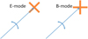 |
Fig. A.1. An illustration of the E and B modes. For each mode, only two polarization directions (arms of the cross) are allowed in respect to the normal vector (arrow). Only one radial direction is plotted as example, and a complete E or B mode is made up of all its rotations. Therefore both E and B modes are rotationally invariant by design. |
Appendix B: Illustration for the loop magnetic field and projection
Figure B.1 illustrates how the loop magnetic field affects the polarization observation, in which S is the center of the supernova remnant, P is one point on the shell, O is the observer, N is an auxiliary point above the paper with NP being perpendicular to the paper, and AB and XY are auxiliary lines that are perpendicular to the line-of-sight and radial direction of the supernova, respectively. For point P on the shell, due to the shell expansion, the magnetic field lines are suppressed and form along the shell; they should therefore be perpendicular to the normal vector PS . This allows two magnetic field components along PN and PY , respectively. The PN component is parallel to the tangent direction of the projected loop on the two-dimensional sky, and is therefore the one discussed in this paper. The PY component can be decomposed into two components along PO and PB , respectively.
 |
Fig. B.1. Illustration on how the polarized loop signal is projected. S is the supernova, O is the observer, P is one point on the shell, AB is perpendicular to OP , and XY is perpendicular to SP . N lies above the paper and NP is perpendicular to the OPS plane. |
The background interstellar magnetic field before the SN explosion can have both regular (smooth) and turbulent components; see for example Beck et al. (1996). The smooth component is expected to have only large-scale variation, while the turbulent component is expected to have random fluctuation at small scales. The threshold for “large-scale” and “small-scale” is not absolutely defined, but in this work, it is assumed that the smooth component has negligible variation at the size of an SN bubble, whereas the turbulent component has random directions in the bubble volume. In this context, their respective contributions are discussed below.
B.1. Contribution of the smooth background magnetic field
As mentioned above, the smooth component will be suppressed by the supernova, and the PS component will be erased. The PO component is therefore aligned with the line-of-sight (LOS), which can not generate any visible polarization (but is related to the Faraday rotation). The contribution of the PB component is projected from the PY component by a factor of sin(θ), which is already suppressed. Furthermore, since the LOS will cross a shell twice, at P and P′, the PB components at these two points will cancel each other out, which means a further cancellation. Therefore, after projection and LOS integration, the major component of the magnetic field that is effective for polarization is the PN component. However, the PB component after suppression and cancellation can be small but non-zero, which might be a source of the B-mode emission from loops.
A complete calculation of the LOS integration in case of smooth background magnetic field is very difficult. Therefore, a much-simplified toy model is provided for example, with the following assumptions/simplifications:
-
The observer stays at [x, y, z] = [0, 0, 0], the center of SN is [0, 0, 1], and the coordinate of P is [R sin(θ) cos(φ), R sin(θ) sin(φ), R cos(θ)].
-
The SN will only erase the PS component.
-
The background magnetic field (before SN explosion) is B = [sin(θ 1) cos(φ 1), sin(θ 1) sin(φ 1), cos(θ 1)], whose direction is uniformly distributed on the sphere. However, for one realization, B is a constant vector.
Therefore, the effective magnetic field along
PN
and
PB
at point P are:![Mathematical equation: $$ \begin{array}{l}{B_{{\rm{PN}}}}\, = \sin ({\theta _1})\sin (\delta )\\ {B_{{\rm{PB}}}}\, = \frac{{R - \cos (\theta )}}{{1 + {R^2} - 2R\cos (\theta )}}[R\cos ({\theta _1})\sin (\theta )\, + (1 - R\cos (\theta ))\cos (\delta )\sin ({\theta _1})], \end{array}\ $$](/articles/aa/full_html/2018/09/aa33471-18/aa33471-18-eq18.gif) (B.1)
(B.1)
where δ = φ 1 − φ.
The polarization angle is bound with the magnetic field, and so are the Stokes parameters. Therefore, Eq. (B.1) gives the following Stokes parameters: (B.2)
(B.2)
Here, according to the coordinate system shown in Fig. B.1, the Q Stokes parameter corresponds to the E-mode, and the U Stokes parameter corresponds to the B-mode.
Apparently, if B PN or B PB is zero, then U(R, θ, θ 1, δ) ≡ 0, and the signal is pure E-mode. Since B PN is a constant in the LOS integration, this provides a good example: if the smooth background magnetic field is along OS (so θ 1 = 0), then the final polarization signal is always pure E-mode.
For an LOS integration, the amplitude of the (Q, U) Stokes parameters is assumed to be scaled by (B.3)
(B.3)
where 1 + R
2 − 2R cos(θ) is the length of
PS
, and γ ≥ 0 is a free parameter that describes the decay of the SN signal according to the shell radius (this is a simplified assumption). Therefore, the integrated stoke parameters along the LOS are: (B.4)
(B.4)
With Eq. (B.4) and various values of θ, θ 1, δ, one can calculate the ratio ρ(θ, θ 1, δ) between the two components, which is exactly the EB-ratio at the given sky direction after LOS integration. With various parameters this ratio can either be greater or smaller than 1. For statistical purposes, uniformly distributed sky directions are assumed for the LOS, the initial magnetic field runs 104 simulations, and the median EB-ratio is roughly 1.7, which moderately prefers the E-mode.
To roughly illustrate the expected EB-ratio ρ(θ, θ 1, δ) for various choices of the parameters, log10(|ρ|) is plotted as function of θ, θ 1 and δ in Fig. B.2, and in each panel the unplotted parameters are simply random. I note that the results are not sensitive to γ. One can see that the E-mode is apparently preferred for θ around 75°, and is moderately preferred for all θ 1. There is also significant sinusoidal modulation associated with the δ parameter with peaks around δ = 0°, 90°, 180° … However, it must be emphasized that Fig. B.2 is only statistical, which cannot cast effective constraints on a specific realization.
 |
Fig. B.2. Logarithm EB-ratio log10(|ρ|) in case of smooth background magnetic field, and as function of θ (left), θ1 (middle) and δ (right). The unplotted parameters are random for each panel. The red lines are for ρ = 1, so the dots above the red line have higher E-mode, and the dots below the red line have higher B-mode. I note that the results are not sensitive to γ. |
B.2. Contribution of the turbulent background magnetic field
The turbulent magnetic field is expected to have random directions for different parts of the sky; however, due to the supernova explosion, the magnetic field components along the
PS
direction are erased, and the magnetic field is constrained within the
NPY
plane with uniformly distributed directions, which can be represented in a circular form: (B.5)
(B.5)
where u 0 is the magnetic field component along the PN direction, υ 0 is the component along the PY direction, φ is the random phase angle in the NPY plane, and |B| is the amplitude of the magnetic field.
For the region around P, the contribution of the turbulent magnetic field can be regarded as the integration of Eq. (B.5) with uniformly distributed φ. Considering the projection from the
NPY
plane to the
NPB
plane that is perpendicular to the LOS, Eq. (B.5) changes from circular to elliptical: (B.6)
(B.6)
where u is the magnetic field component along the
PN
direction, υ is the component along the
PB
direction, ψ is the phase angle of the polar system in the
NPB
plane, and |B′| is the amplitude of the effective magnetic field after projection. The polarization angle is simply ψ′ = ψ + 90°; therefore, for the synchrotron emission, the integrations of the Q, U Stokes parameters for the region around P are: (B.7)
(B.7)
As mentioned already in Appendix B.1, here the Q Stokes parameter represents the E-mode, and the U-Stokes parameter represents the B-mode. Therefore, one can see that the turbulent magnetic field always gives pure E-mode.
The physical meaning of Eq. (B.7) is: due to the “2ψ” rule of the polarization angles, the symmetry of the integral along the ellipse is broken, so the two directions separated by π no longer cancel each other, which is the source of non-zero E-mode. If 2ψ′ is replaced by ψ′ in Eq. (B.7), then both integrals are zero.
With Eq. (B.7), the conclusion is apparent: supernova explosion plus a turbulent background magnetic field will produce pure E-mode in the polarized signal. However, it is always possible that, due to asymmetry of the supernova explosion, the B-mode is small but non-zero.
Appendix C: Note added to proofs – updated table with the Planck final data release
During the production stage of this paper, Planck released its final results8, which is used to update Table 2. The new results are listed in Table C.1. The Planck final data release is expected to have lower systematics, and one can indeed see that the blue regions in Table 2, which were marked as suspicious due to systematics, become apparently lower in Table C.1, which makes the conclusions in this work more robust.
Same to Table 2, but the Planck results are updated with the Planck final data release.
All Tables
List of 〈δ θ 〉 in degrees between the minimal Loop I model and 23–353 GHz bands.
Same to Table 2, but the Planck results are updated with the Planck final data release.
All Figures
|
Fig. 1. Upper left: example of the expected loop polarization directions (by small black lines). Upper right: polarization directions of the WMAP K-band in the Loop I region, with Loop I marked by a black circle. The color scales of the upper panels are for the polarized intensity, which is 0 ~100 μK for the K-band and −1 ~ 1.2 for the model (here the absolute amplitude of polarization intensity is meaningless for the model, and therefore such an unphysical range is chosen to maximize the visibility of the thin lines). Lower: the angular power spectrum of the model shown in upper-left, calculated without a mask. We note that the polarization directions in the model are strictly along the normal vectors, and some small misalignments are only visual effects due to pixelization. |
| In the text | |
|
Fig. 2. Polarization intensity maps and their EB decompositions at the K-band (upper) and 353 GHz (lower). From left to right: total polarized intensity P, P E, and P B. The loop-like structures are marked by black or white lines depending on visibility. They are apparently visible in E-mode (middle) but disappear in B-mode (right). |
| In the text | |
|
Fig. 3. Ratio ρ = P E/P B in K-band (upper) and 353 GHz (lower), both full sky and around the same arches as marked in Fig. 2. The outline of the BICEP2 zone is marked in thick dash line. |
| In the text | |
|
Fig. 4. Left: polarization angles calculated from the minimal model, with no free parameters and no fitting. Middle: the real data (WMAP K-band). Right: real data and only E-mode. The color-to-angle mapping is given by the low-left color disk,and the black circle is the critical range that is 90° from the center of Loop I. |
| In the text | |
|
Fig. 5. Regions used to estimate the significance of the model-to-data association, where red means usable region and green means masked region. Left: the region used in Sect. 3.2. Middle and right: the inside and outside regions used in Sect. 3.3, which are 0°–90° and 90°–120° to the center of Loop I, respectively. The BICEP2 region is also marked in each panel. |
| In the text | |
|
Fig. 6. Histograms of 105 mean angle differences 〈δ θ 〉 between the minimal model and simulations, on which results from the real data are marked by thin vertical lines, and the 45° expectation of 〈δ θ 〉 is marked by the central vertical line. |
| In the text | |
|
Fig. A.1. An illustration of the E and B modes. For each mode, only two polarization directions (arms of the cross) are allowed in respect to the normal vector (arrow). Only one radial direction is plotted as example, and a complete E or B mode is made up of all its rotations. Therefore both E and B modes are rotationally invariant by design. |
| In the text | |
|
Fig. B.1. Illustration on how the polarized loop signal is projected. S is the supernova, O is the observer, P is one point on the shell, AB is perpendicular to OP , and XY is perpendicular to SP . N lies above the paper and NP is perpendicular to the OPS plane. |
| In the text | |
|
Fig. B.2. Logarithm EB-ratio log10(|ρ|) in case of smooth background magnetic field, and as function of θ (left), θ1 (middle) and δ (right). The unplotted parameters are random for each panel. The red lines are for ρ = 1, so the dots above the red line have higher E-mode, and the dots below the red line have higher B-mode. I note that the results are not sensitive to γ. |
| In the text | |
Current usage metrics show cumulative count of Article Views (full-text article views including HTML views, PDF and ePub downloads, according to the available data) and Abstracts Views on Vision4Press platform.
Data correspond to usage on the plateform after 2015. The current usage metrics is available 48-96 hours after online publication and is updated daily on week days.
Initial download of the metrics may take a while.