| Issue |
A&A
Volume 694, February 2025
|
|
|---|---|---|
| Article Number | A198 | |
| Number of page(s) | 12 | |
| Section | Cosmology (including clusters of galaxies) | |
| DOI | https://doi.org/10.1051/0004-6361/202452588 | |
| Published online | 14 February 2025 | |
Forecasts of effects of beam systematics and deprojection on the third-generation ground-based cosmic microwave background experiment
1
Department of Astronomy, University of Science and Technology of China, Chinese Academy of Sciences, Hefei, Anhui 230026, People’s Republic of China
2
School of Astronomy and Space Sciences, University of Science and Technology of China, Hefei 230026, People’s Republic of China
3
Dipartimento di Fisica, Università degli Studi di Torino, Via P. Giuria 1, 10125 Torino, Italy
4
INFN – Istituto Nazionale di Fisica Nucleare, Sezione di Torino, Via P. Giuria 1, 10125 Torino, Italy
5
Institute for Frontier in Astronomy and Astrophysics, Beijing Normal University, Beijing 102206, People’s Republic of China
6
Department of Astronomy, Beijing Normal University, Beijing 100875, People’s Republic of China
⋆ Corresponding authors; doujzh@mail.ustc.edu.cn; wzhao7@ustc.edu.cn; bhu@bnu.edu.cn
Received:
12
October
2024
Accepted:
29
December
2024
The ground-based cosmic microwave background (CMB) experiments are susceptible to various instrumental errors, especially for B-mode measurements. The difference between the response of two polarized detectors, referred to as the beam mismatch, would induce a T → P leakage when the detector pair is differenced to cancel the unpolarized signal. We applied the deprojection technique on the time-ordered mock data to mitigate the systematic contamination caused by beam mismatches by assuming the third-generation ground-based CMB experiment (S3). Our results show that the deprojection effectively recovered the input power spectra. We adopted the Needlet ILC (NILC) and constrained ILC (cILC) methods to reconstruct the foreground-cleaned TEB maps, and we evaluated the level of residual systematic errors after the foreground cleaning pipeline by comparing the power spectra between the systematics-added data after deprojection and the systematics-free data. The results show that the residual beam systematics cleaned by deprojection do not bias the CMB measurements of the T, E, and B modes nor the CMB lensing reconstruction or the estimation of the tensor-to-scalar ratio under the S3 sensitivity.
Key words: gravitational lensing: weak / instrumentation: detectors / cosmic background radiation
© The Authors 2025
 Open Access article, published by EDP Sciences, under the terms of the Creative Commons Attribution License (https://creativecommons.org/licenses/by/4.0), which permits unrestricted use, distribution, and reproduction in any medium, provided the original work is properly cited.
This article is published in open access under the Subscribe to Open model. Subscribe to A&A to support open access publication.
1. Introduction
Precise measurements of cosmic microwave background (CMB) polarization are particularly essential for modern cosmology and for exploring new physics beyond the ΛCDM model (Planck Collaboration VI 2020). The detection of the primordial B-mode polarization would reveal the mystery of the cosmic inflation era. The amplitude of the primordial B modes is commonly described by the ratio of the tensor power spectrum to the scalar power spectrum at some pivot scale, called the tensor-to-scalar ratio. Successive ground-based CMB experiments over the past decade have made great efforts to increase their sensitivities to enable a significant detection of the tensor-to-scalar ratio, such as BICEP/Keck Array (BICEP/Keck Collaboration 2021), the Atacama Cosmology Telescope (ACT) (Louis et al. 2017), the Cosmology Large Angular Scale Surveyor (CLASS) (Essinger-Hileman et al. 2014; Harrington et al. 2016), and the South Pole Telescope (SPT) (Sayre et al. 2020). The current best constraint on the tensor-to-scalar ratio is r < 0.032 (95% C.L.) and was obtained from the combination of Planck, BAO, and BICEP/Keck data (Tristram et al. 2022). Future CMB experiments such as the Ali CMB Polarization Telescope (AliCPT) (Li et al. 2019; Li et al. 2018), the Simons Observatory (Simons Observatory Collaboration 2019), the Q&U Bolometric Interferometer for Cosmology (QUBIC) (Mennella et al. 2019), LiteBIRD (Hazumi et al. 2019), and CMB-S4 (Abazajian et al. 2016, 2022; CMB-S4 Collaboration 2022) will continue to pursue the target of higher sensitivities on constraining r.
Precise measurements of the CMB polarization are challenging not only because it is weaker than the instrumental noise, but also because of complicated contaminants from astrophysics and instruments. Diffuse galactic foregrounds such as synchrotron and thermal dust emit strong polarized radiation at microwave frequency bands with a significant amplitude relative to the CMB polarization signal. Component separation methods are implemented on the multifrequency sky observations to remove the foregrounds (mostly) based on the fact that CMB and foregrounds have different spectral energy distributions (SED). Our imperfect knowledge of the actual optical response of the telescopes results in instrumental systematic effects, such as the unknown difference between the response of two polarized detectors that might transform a fraction of the CMB temperature modes into polarization modes. This is called the T → P leakage. The leakage must be mitigated especially because the temperature modes and the polarization modes peak at similar angular scales so that the leakage of the former has a higher magnitude than the signal of the latter. Additionally, the gravitational lensing effect where the matter field gravitationally deflects the CMB photons can covert part of E modes into B modes at intermediate and small scales, giving rise to lensing B modes that dominate the primordial B modes (Blanchard & Schneider 1987; Zaldarriaga & Seljak 1998). Fortunately, the lensing convergence can be reconstructed using either internal CMB anisotropies or external large-scale structure (LSS) tracers such as galaxy surveys, 21 cm observations, and measurements of the cosmic infrared background (CIB) (Hu 2001; Hu & Okamoto 2002; Okamoto & Hu 2003; Carron & Lewis 2017; Maniyar et al. 2021; Planck Collaboration IV 2020a).
We consider a typical configuration for a small-aperture ground-based CMB telescope. Specifically, we assumed a total of 7000 polarized detectors, evenly split between the 95 GHz and 150 GHz frequency bands. Each detector had a noise equivalent temperature (NET) of  . The full width at half maximum (FWHM) beam sizes were assumed to be 19 arcminutes and 11 arcminutes for the 95 GHz and 150 GHz bands, respectively. This setup reflects the typical design of a third-generation ground-based CMB experiment (S3) (Abazajian et al. 2016). We focus on exploring the impact of the beam mismatch, which is a difference in the beam shape or beam center between the two detectors of a detector pair that leads to the T → P leakage. An analysis technique called the deprojection was exploited to filter this contamination out (BICEP2 Collaboration 2015; Sheehy 2019). We used the deprojection algorithm to handle the time-ordered data (TOD) with the beam systematics, and we evaluated the effects of undeprojected residual systematics on the follow-up steps of our whole pipeline, including component separation, lensing reconstruction, and the estimation of the tensor-to-scalar ratio. The residual systematic error was found to be negligible given the sensitivity of S3.
The paper is organized as follows. In Sect. 2 we first review the formalism of beam mismatches modeled by six coefficients. Then, we introduce our deprojection pipeline to mitigate the systematics induced by beam mismatches. Finally, we summarize the simulations used to assess the effectiveness of deprojection. In Sect. 3 we introduce the foreground cleaning pipelines including Needlet ILC (NILC) and constrained ILC (cILC), which we used to clean the T or E modes and B modes, respectively. We present the results of the mock data after deprojection and foreground cleaning, carry out a lensing reconstruction process on the foreground-cleaned maps, and constrain the tensor-to-scalar ratio r using the cleaned B-mode power spectrum in Sect. 4. Finally, we conclude in Sect. 5.
2. Beam systematics and deprojection
The beam is the response of an antenna to sky radiation as a function of angle. Basically, each pixel on the focal plane includes a pair of two orthogonally polarized antennas that observe the same direction on the sky. The time streams from detectors a and b (a pair) are summed to obtain the total intensity (temperature) measurement, and they are differenced to cancel the unpolarized component. The radiation polarization is measured in this way. The typical beams of S3 are circular Gaussians with FWHM = 19 arcmin for 95 GHz, and 11 arcmin for 150 GHz, where there is no systematics in the ideal case. However, when the beams of the two antennas are mismatched, which means that their instrumental responses are different, the temperature signal is not completely canceled and could induce a spurious polarization signal in the pair difference data of the detector pair1. For the ith detector, the TOD stream reads
![$$ \begin{aligned} \begin{aligned} \tau _i(t)&=g_i\int d\nu \int d\Omega \prime A_i(\nu )B_i[\boldsymbol{\hat{n}}(t)-\boldsymbol{\hat{n}}\prime ] \\&[I\prime _{\nu }(\boldsymbol{\hat{n}}\prime )+Q\prime _{\nu }(\boldsymbol{\hat{n}}\prime )\cos 2\psi _i(t)+U\prime _{\nu }(\boldsymbol{\hat{n}}\prime )\sin 2\psi _i(t)]\;. \end{aligned} \end{aligned} $$](/articles/aa/full_html/2025/02/aa52588-24/aa52588-24-eq2.gif)
Of these, gi is the gain of the detector, Ai(ν) is the response of this detector at different frequencies, and ![$ B_i[\boldsymbol{\hat n}(t) - \boldsymbol{\hat n}{\prime}] $](/articles/aa/full_html/2025/02/aa52588-24/aa52588-24-eq3.gif) is the beam function, representing the spatial response of the detector.
is the beam function, representing the spatial response of the detector.  $](/articles/aa/full_html/2025/02/aa52588-24/aa52588-24-eq4.gif) are the Stokes parameters of the cosmic microwave background radiation at frequency ν and position
are the Stokes parameters of the cosmic microwave background radiation at frequency ν and position  . The terms
  and ψi(t) are determined by the scan strategy. In an ideal case,
  and Ai(ν) are delta functions. The beam systematic errors are included in the following way:
-
The pointing error refers to the deviation between the pointing direction read by the instrument
 and the true pointing direction of the telescope
  .
. -
The band pass mismatch for a pair of detectors a and b means Aa(ν)≠Ab(ν), which can introduce false signals when taking the difference between the readings of the detectors.
-
The beam mismatch for a pair of detectors a and b similarly refers to Ba(r)≠Bb(r), which can also introduce false signals in the detector difference.
-
The gain mismatch arises when ga ≠ gb. Like the previous two points, this can introduce false signals in the detector difference.
-
The detector polarization angle calibration is typically detected by two detectors set to an angle of 90°. However, due to the precision of the detector manufacturing, the preferred polarization angle can deviate, that is, ψa(t)−ψb(t)≠90°, which can introduce systematic errors during the subsequent map-making process.
The first four errors above are all equivalent to an overall miscalibration of the detectors and a differential response between a pair of detectors at the same frequency, where we refer to the latter as beam mismatch in the following. A detector polarization angle miscalibration would introduce the E → B leakage, which is beyond the scope of this work. Given the high amplitude of the CMB temperature anisotropies relative to the polarization signal, the leakage from T to P must be carefully taken into account. The T → P leakage due to beam mismatches can be written as the convolution of the unpolarized signal and the differential beam within a detector pair,
![$$ \begin{aligned} d_{T\rightarrow P}=T(\boldsymbol{\hat{n}})*[B_a(\boldsymbol{\hat{n}})-B_b(\boldsymbol{\hat{n}})]=T(\boldsymbol{\hat{n}})*B_\delta (\boldsymbol{\hat{n}}), \end{aligned} $$](/articles/aa/full_html/2025/02/aa52588-24/aa52588-24-eq10.gif)
where  refers to the temperature anisotropies,
  and
and  are the beams of two detectors, and
  is the differential beam of the pair.
As in BICEP2 Collaboration (2015) (hereafter BKIII), we modeled  as the difference of two elliptical Gaussian beams for simplicity. This can be parameterized by six parameters (or differential modes): the gain difference δg, the differences of the pointing center coordinates (with respect to the nominal beam center) δx and δy, the Gaussian beam-width difference δσ, and the differences of the plus- and cross-ellipticity δp and δc. The plus-ellipticity describes an ellipse whose major axis is oriented horizontally or vertically, and the cross-ellipticity describes an ellipse whose major axis is oriented ±45° with respect to the x-axis (see more details in BKIII, Appendix A). For each differential mode k = {g, x, y, σ, p, c}, δk = ka − kb is the difference of the beam parameter between two detectors.
  is the linear combination of the beams of the six modes, where each mode independently produces a pattern of the spurious polarized signal, also called a leakage template. For instance, since the beam of differential gain
  is simply the scaled version of the circular Gaussian beam, its leakage is the scaled version of the beam-smoothed temperature
  according to Eq. (2). Under the assumption that the mismatch is small, except the third and higher orders, all the templates are the beam-smoothed map of
  and its first and second spatial derivatives (see Table 1) (Hu et al. 2003). The map-making procedure is a linear operation, meaning that the total leakage is the linear combination of the leakage templates of these differential modes. Therefore, we filtered the leakage out by fitting these templates to our data and then subtracting them.
Six beam mismatch parameters added to the mock TOD and the corresponding leakage templates.
The leakage templates we used are from the Planck 100 and 143 GHz reobserved TOD, which we used to clean 95 and 150 GHz, respectively. The reobserved templates were produced as follows:
-
We first generated CMB, foreground, and noise simulations of the Planck HFI bands as introduced below.
-
We coadded all components and reconvolved the coadded sky maps with the S3 nominal beams. For Planck 100 GHz, we divided aℓm by the 100 GHz beam function and then multiplied them by the S3 95 GHz Gaussian beam. (This can be done on the input maps since the Planck and S3 nominal beams are circularly symmetric.)
-
We computed the first and second derivatives of the Planck T maps2.
-
We rescanned the T maps and their derivatives for each HFI band using the same pointing matrix as in S3.
For the realistic observations, we reobserved the PR4 (NPIPE) maps (Planck Collaboration Int. LVII 2020) using the S3 scan strategy. Our templates contained the noise component of the Planck HFI bands, which is not involved in the true T → P leakage, but we assumed that the noise is much lower than the temperature signal. We produced simulated S3 TOD from the CMB-plus-foreground coadded maps using Eq. (1), and we computed the pair-difference time stream of the TOD by differencing the a and b detector time streams within a pair: τdiff(t) = (τa − τb)(t)/2. We finally fit the templates to the pair difference TOD and subtracted the fitted templates. Noise is not involved in the data since we expect that the noise is uncorrelated to the templates from Planck HFI maps, and the separation of noise ensured clearer analyses of the different components in the following foreground-cleaning pipeline.
The assumed S3 experiment is located in the northern hemisphere. In its first observing season, it will scan 17% of the sky where the thermal dust emission is clean, centering at RA = 170° and Dec = 40° in the celestial coordinate system. The polarized maps have a map depth of about 18 μK-arcmin at 95 GHz and 24 μK-arcmin at 150 GHz.
Our mock dataset consisted of 300 simulated sky maps at Nside = 1024 in seven frequency bands, including the 95 and 150 GHz dual bands, the Planck HFI 100, 143, 217, 353 GHz bands, and the WMAP K band. The additional Planck and WMAP channels were for the purpose of cleaning the foregrounds more thoroughly. Each of the sky maps contained CMB, foregrounds, and white noise. First, we drew the six ΛCDM cosmological parameters within one standard deviation of the Planck 2018 best-fit cosmological constraints (Planck Collaboration VI 2020), from which we generated the lensed CMB power spectrum by CAMB (Lewis et al. 2000). The CMB realizations were generated from the lensed power spectrum with the tensor-to-scalar ratio r = 0, using the synfast facility from lenspyx (Reinecke et al. 2023). The Galactic foregrounds containing thermal dust, synchrotron, free-free, spinning dust, and CO emissions were produced using the Planck Sky Model (PSM) package (Delabrouille et al. 2013), which is the same as the foregrounds used in previous papers (Dou et al. 2024; Han et al. 2023b). The thermal dust polarization maps were generated by scaling the Planck 2018 GNILC polarized-dust template (Planck Collaboration IV 2020) to different frequencies using a modified blackbody SED with the dust temperature and spectral indices adopted from the best fit of the Planck 2015 GNILC dust maps (Planck Collaboration Int. XLVIII 2016). The synchrotron polarization template was based on the Planck 2018 SMICA map and was scaled by a power-law SED with a fixed βs of −3.08. We did not use the current best-fit values to avoid confirmation biases during foreground removal. For the 95 and 150 GHz bands alone, we generated the TOD simulations of CMB plus foregrounds following Eq. (1) and the S3 scan strategy, where we assumed the stochastic beam mismatch parameters whose mean and uncertainty are listed in Table 1. The values were chosen to be at the same level as the measured beam parameters of the BICEP2 instruments (BICEP2 Collaboration 2014; BICEP2/Keck Collaboration 2015). They measured the beam shape parameters for each detector using a chopped thermal source mounted on a mast, and calibrated the differential gains using the cross-correlation of temperature maps for individual detectors with Planck. We created white-noise simulations assuming that the realistic 1/f noise can be significantly removed by pair differencing and TOD polynomial filtering (BICEP2 Collaboration 2014). The white-noise simulations unrelated to systematics were generated from the noise covariance matrices of the S3 and WMAP-K bands (Bennett et al. 2013). For the Planck HFI bands, we adopted 300 FFP10 noise simulations from the Planck Legacy Archive3. The deprojection process was performed on the CMB-plus-foreground data assuming that the effects on the noise component are negligible.
3. Foreground-cleaning pipeline
We implemented the same foreground-cleaning methods as Han et al. (2023b) to qualify the deprojection performance on the foreground-cleaned maps. The T and E modes were cleaned by the NILC method, and the B modes were cleaned by the cILC method because the foreground dominates the B-mode signal.
The maps after foreground cleaning (NILC or cILC) consisted of four ingredients: the CMB signal, the residual foregrounds, the residual noise, and the systematic residual. For the purpose of examining the efficacy of the foreground cleaning methods, each component in the output map can theoretically be obtained by projecting ILC weights on the maps of the input component, given the linearity of ILC methods. However, the input CMB and foregrounds are mixed up during deprojection so that the systematic contamination on the CMB and foregrounds can never be separated afterward. Instead, we first subtracted the residual noise from the total residual (the foreground-cleaned map minus the input CMB map), which was the sum of the residual foregrounds and the systematic residual. We then projected the ILC weights on the deprojection residual maps at the 95 and 150 GHz bands to obtain the deprojection residual in the foreground-cleaned maps. Finally, we subtracted it from the sum to compute the residual foregrounds.
3.1. The NILC pipeline
The needlet internal linear combination (NILC) method (Delabrouille et al. 2009; Basak & Delabrouille 2012, 2013) is a widely used blind component-separation technique that linearly combines the raw data from different frequencies while minimizing the variance in the needlet space. Needlets are a special form of wavelets that permit a localization in harmonic and real (pixel) space. They are therefore suitable for component separation when the properties of the sky components vary significantly with the sky positions and scales. We adopted the NILC method for cleaning foregrounds in T- and E-mode maps, the details of which are described below.
The sky observations dν(p) at a frequency band ν and sky pixel p were first transformed into spherical harmonic coefficients using HEALPix4 (Gorski et al. 2005): dℓmν = ∫dν(p)Yℓm*(p)dΩ. The raw maps with different beams were then reconvolved into the common resolution by  , where bℓ is the beam transfer function. The common beam resolution (bℓout) was chosen as a Gaussian beam with FWHM = 11 arcmin, which is the resolution of the 150 GHz band. For the WMAP K band and 95 GHz, which have larger beam sizes than the common beam (bℓin < bℓout), we cut off the harmonic coefficients of these two bands with ℓ greater than 350 and 1200, respectively, to avoid an overamplification of the instrumental noise. The harmonic coefficients can be decomposed into a set of filtered maps,

where the needlet bands hℓj satisfy ∑j(hℓj)2 = 1, defining a localization scheme in harmonic space. We adopted the cosine needlet bands as shown in Fig. 1 of Han et al. (2023b). The eight needlet bands peak at 15, 30, 60, 120, 300, 700, 1200, and 2000 with ℓmax = 2000. For the WMAP K band, whose coefficients with ℓ > 350 were cut off, the needlets whose peaks (ℓpeak) are greater than 350 would not be applied to the K-band data (and so is for 95 GHz band). For each frequency band, the filtered maps were then transformed back to real space, forming a set of needlet maps. The needlet coefficient of the jth needlet and the kth pixel after transformation is given by
where Nj denotes the number of pixels of the jth needlet map, and  denotes the pixel center of the kth pixel of the jth needlet map.
When the data were transformed to needlet space, we applied the internal linear combination method to the multichannel data. First we estimated the data covariance matrix across the frequencies by averaging the needlet coefficient product  over a disk of pixels centered at pixel k. The empirical data covariance between ν1 and ν2 is written as
where wj(k, k′) are the weights that select the region around a pixel k to average out, and nk is the number of selected pixels. The NILC solution is a linear combination of the needlet coefficients of all frequencies,
where the NILC weights are given by
![$$ \begin{aligned} w^\mathrm{NILC}_{\nu , j}(\hat{p}_{jk}) = \left[\frac{\boldsymbol{\hat{C}}_{jk}^{-1} \boldsymbol{a}}{\boldsymbol{a}^t\boldsymbol{\hat{C}}_{jk}^{-1} \boldsymbol{a}}\right]_\nu \,. \end{aligned} $$](/articles/aa/full_html/2025/02/aa52588-24/aa52588-24-eq35.gif)
Here,  is the nν × nν empirical data covariance matrix, where nν is the number of frequency channels, and a is the spectral response vector that characterizes the variation in the signal with frequencies. Because the CMB signal is frequency independent in thermodynamic temperature units, we set a as a unit column vector with a length of nν. The relation
  ensures the precise recovery of the CMB component.
Finally, we performed an inverse needlet transformation to obtain the NILC-cleaned map,
The recovered CMB map in real space is given by  . We used a mask that preserved the pixels with a noise variance of the 150 GHz band smaller than 20 μK pixels, whose sky fraction was about 10% (see Fig. 2).
3.2. The cILC pipeline
Following the ILC method, the constrained ILC (cILC) method (Remazeilles et al. 2011, 2021) was developed to further mitigate the residual foreground contaminants by adding constraints on the ILC weights. We used the cILC method in harmonic space to produce foreground-cleaned B-mode maps because the foregrounds are several orders of magnitude higher than the CMB signal for B modes, and the standard ILC method is therefore insufficient to reduce the residual foregrounds to a level of r = 0.01 primordial tensor modes under the sensitivities of S3.
We modeled the B-mode observation at a frequency ν and pixel p as the sum of nc sky components and the thermal noise,
where sc(p) is the astrophysical emission template of component c, and nν(p) is the noise. The nν × nc mixing matrix A stores the spectral response information that describes the SED of component c at frequency ν. In our implementation, we only considered three dominant sky components: the lensed CMB, the polarized thermal dust, and the polarized synchrotron. The first column of the mixing matrix refers to the mixing vector of CMB, a. The second column corresponding to dust emissions was calculated assuming a modified blackbody SED with fixed Tdust = 19.6 K and βdust = 1.59. The third column, that is, the mixing vector of the synchrotron, follows the power law SED with fixed βsync = −3 in Rayleigh-Jeans brightness temperature units.
The cILC weights are given by
which satisfy the constraints of nulling the foreground components (dust and synchrotron),
where e is a row vector with length nc, whose element ec is one for the CMB and zero for the foreground components. The empirical data covariance matrix  is computed by
where ℓmin = min[0.6ℓ,ℓ−7], and ℓmax = max[1.4ℓ,ℓ+7], and we excluded the center multipole (ℓ′≠ℓ) to mitigate the ILC bias. The input maps were reconvolved to a common beam of 11 arcmin. The analysis was performed with ℓmax = 2000, while the harmonic coefficients of WMAP-K and 95 GHz bands were not involved as ℓ is greater than 350 and 1200, respectively. The cILC-cleaned CMB map was finally obtained by  . To reduce the foreground contaminants, we used a smaller mask (fsky ≈ 7%) to clean the B maps, which was produced by removing the pixels with a noise variance in the 150 GHz band larger than 10 μK-pixel and a declination above 65° (see the third row of Fig. 4).
4. Results
In this section, we detail the results of the fitted beam parameters from deprojection and the deprojected maps of the S3 dual bands. We then combine the S3 channels with four Planck HFI channels and WMAP K band in the foreground-cleaning pipeline to extract the CMB signal, and we reconstruct the lensing potential power spectrum from the foreground-cleaned maps. We finally evaluate the impacts of the systematic residual on the CMB power spectra, lensing potential, and the tensor-to-scalar ratio r.
4.1. Deprojection results
The assumed S3 telescope contains 1728 detector pairs on the focal plane for the 95 and 150 GHz bands, with a field-of-view width ∼30°. We considered one observing season (lasting about half a year), which was divided into 3183 scansets (each lasting roughly 30 minutes). A scanset covers tens of constant elevation scans (CES) that the telescope operates from one end to the other at a speed of ∼4° /s. Between the scansets, the telescope makes elevation nodding (elnod) scans to calibrate the relative gains of the detectors. We generated time streams from the simulated CMB plus foregrounds following the S3 scan trajectory. We derived the six leakage templates from the Planck simulations as described in Sect. 2. Although the input beam parameters are constant with time, we fit the time-ordered templates to the S3 TOD every 30 scansets for each detector pair to account for the time-varying beam systematics in realistic instruments. The histogram of the fitted beam mismatch parameters of 106 time chunks for one detector pair of a realization at 150 GHz is shown in Fig. 1. The scatter across time slices would be averaged in the map-making process, and the deviation of the mean from the true values (input parameters) due to noise fluctuations in templates leads to the undeprojected residual.
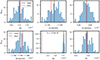 |
Fig. 1. Distribution of the recovered beam mismatch parameters of 106 time trunks for one detector pair of a noise-free simulation at 150 GHz. The dashed red lines represent the input beam parameter, and the dashed black lines indicate the mean over all time series. There is a bias on the differential plus-ellipticity of Δ ≈ 7.3 × 10⁻³ due to the cosmological TE correlation. |
We note a systematic bias on the recovered differential plus-ellipticity δp at a level of Δ = δprecov − δpinput ≈ 7.3 × 10⁻³. Due to the CMB-inherent TE correlation, the deprojection template of δp correlates with the polarized signal in the pair-difference time stream, resulting in a bias on the deprojection coefficient even when it is free of beam systematics (BICEP2 Collaboration 2015). This bias does not impair the filtering of T → P leakage, but leads to an additional filtering of cosmological E modes (the effects on the B modes are negligible). We corrected for the bias using the averaged deprojection coefficient estimated from systematics-free simulations, which is ⟨δprecov⟩ = 7.2 × 10⁻³⁵. We also checked the strong correlation between the time-averaged recovered coefficients and the input coefficients for all detector pairs in Appendix A.
Finally, we subtracted the fitted templates from the pair difference data for all time trunks of detector pairs. We simplified the map-making process by averaging the time streams of detectors pointed at each map pixel and adding white-noise maps to obtain the observed sky maps.
4.2. Frequency maps
We performed the deprojection procedure on CMB-plus-foregrounds TOD with beam systematics of the S3 95 and 150 GHz bands and implemented the map-making to obtain the frequency maps. The 150 GHz B-mode maps before and after the deprojection pipeline are plotted in the first row of Fig. 2, where the left plot shows the input CMB plus foregrounds without beam systematics, the middle plot shows the CMB plus foregrounds with beam systematics, and the right plot shows that after deprojection. The beam systematics with the level considered in this work only substantially affect the B modes, which induce a spurious signal mainly at small scales. The deprojection residual maps shown in the second row of Fig. 2 illustrate that the deprojection can recover the input T-, E-, or B-mode signal. The deprojection has no effect on the T modes, but the noise fluctuation in the deprojection template may lead to a residual T-to-P leakage on the E and B modes. However, our results show that the residual leakage almost vanishes in deprojected maps.
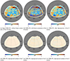 |
Fig. 2. Maps of CMB plus foregrounds at S3 150 GHz. First row: Input B-mode CMB and foregrounds without beam systematics (left), CMB plus foregrounds with beam systematics (middle) and after deprojection (right). Second row: Difference between the deprojected map and the input map without beam systematics for the T (left), E (middle), and B (right) modes. The results of 95 GHz are similar to the 150 GHz results. |
We used the PCL-TC estimator (as detailed in Appendix B) to estimate the power spectra of 150 GHz maps, as shown in Fig. 3. The band powers have a multipole bin size of 30 and ℓmax = 700. Only in the BB power spectrum can the beam systematics bias the power spectrum of input CMB plus foregrounds significantly, while the power spectra of deprojected maps for all modes fit the input spectra well. The residual after deprojection (plotted as the dashed cyan curve) for BB is about 2∼3 orders of magnitude lower than the input CMB plus foreground power spectrum (solid black curves).
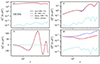 |
Fig. 3. TT, EE, TE, and BB power spectra of the 150 GHz CMB plus foregrounds map with beam systematics before (blue curves) and after deprojection (red curves) for one realization. The input CMB+FG. power spectrum without beam systematics is shown as a solid black curve for comparison with the deprojected one, and their difference, the residual after deprojection, is shown as a dashed cyan curve. The results of 95 GHz are similar to the 150 GHz results. |
4.3. Foreground-cleaned maps
After propagating the maps with beam systematics through the deprojection pipeline, we used the NILC method to clean the foregrounds of T- and E-mode maps and used the cILC approach to clean the B-mode maps. The cleaned maps are plotted in Fig. 4. The left column shows the input CMB maps without adding beam systematics, the middle column shows the NILC-cleaned T and E maps from seven bands, and the right column shows the difference between the cleaned map and the input CMB. The residual maps are dominated by the noise fluctuation for the B modes, while the NILC maps for the T and E modes are dominated by signal.
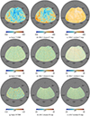 |
Fig. 4. Maps of the input CMB (left column), the foreground-cleaned maps (middle column), and their difference, i.e., the residual maps (right column) for the T, E, and B modes. The first row shows T maps, the second row shows E maps, and the third row shows B maps. |
For the B modes, we computed the systematic residual map by projecting the cILC weights on the 95 and 150 GHz deprojection residual maps plotted in Fig. 2. In this way, we separated the three components in the B-mode cILC residual map from each other, as shown in Fig. 5. The small-scale artifacts in the systematic contamination map are clearly visible. The residual on the boundaries would be removed through mask apodization in the power spectrum estimation.
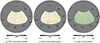 |
Fig. 5. cILC residual B maps of the systematics (left), foreground (middle), and noise (right) components for one realization. |
The power spectra of the NILC- and cILC-reconstructed maps are shown in Fig. 6. The orange curves refer to the residual noise power spectrum obtained from projecting the NILC or cILC weights on the input noise maps. The green curves, as mentioned in Sect. 3, represent the sum of the foreground and beam systematic residuals. For the B modes, the two contaminant components are separately plotted as red and purple curves. The foreground residual dominates the systematic residual at large scales (ℓ ≲ 300). The deprojection residual is negligible compared to the CMB B-mode power spectrum at all scales. Our foreground cleaning methods are sufficient to recover the CMB signal, and the residual contaminants remain much lower than the reconstructed CMB power spectrum for the T and E modes and lower than the noise fluctuation for the B modes.
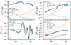 |
Fig. 6. Power spectra including NILC-cleaned TT (left top), NILC-cleaned EE (right top), NILC-cleaned TE (left bottom), and cILC-cleaned BB (right bottom) power spectra with ℓmax = 1500. The input CMB (solid black curves), the reconstructed CMB (blue bars), and the residual noise (orange curves) power spectra are plotted in each panel. The green curves represent the sum of the systematic and foreground residuals. For the BB spectra, the deprojection and foreground residuals are separately shown as red and purple curves, respectively. The power spectra are binned over every 30 multipoles except for the BB spectra, where a logarithm binning at ℓ > 100 was adopted for clarity. |
4.4. Lensing reconstruction
In addition to the primordial B-mode signal, S3 can also detect the lensing signal with a moderate significance because the noise performance is excellent. In what follows, we evaluate the systematic effects on the lensing reconstruction by using the simulated 4 modules*yr data. We fed the 301 simulation sets mentioned above through the lensing pipelines (Carron & Lewis 2017; Liu et al. 2022a; Han et al. 2023a) and tested their performance.
In the presence of lensing-induced correlations among different multipole moments, the off-diagonal terms of the covariance matrix of the CMB fields become nonzero. This allowed us to calculate the quadratic estimator (Hu & Okamoto 2002; Okamoto & Hu 2003) using pairs of filtered maps in their quadratic form (Carron & Lewis 2017; Maniyar et al. 2021), as described in Eqs. (3.4) to (3.8) of Liu et al. (2022b). In this approach, one map in the pair is Wiener filtered, while the other is inverse-variance filtered. To mitigate biases introduced by random disconnected noise, masking effects, and foreground residuals, we employed a Monte Carlo simulation method to estimate these contributions and performed a mean-field subtraction by averaging over the quadratic estimators, using 60 simulation sets.
Normalization was conducted in two stages: We first assessed the averaged noise level for the entire mock dataset and computed the normalization factor analytically, assuming an effective isotropic noise level. Then we corrected for normalization bias arising from noise inhomogeneities through numerical simulations. The raw power spectrum of the lensing is simply
where  denotes the harmonic transformation of the reconstructed lensing potential. However, the outcome of the quadratic estimator contains not only the lensing potential signal, but also the Gaussian reconstruction noise sourced by the CMB and instrumental noise (N0 bias) and the nonprimary couplings of the connected four-point function (Kesden et al. 2003) (N1 bias). We calculated the realization-dependent N0 bias (RDN0) using 240 simulation sets, while the N1 bias was calculated analytically. After subtracting these biases, we obtained the final estimated power spectrum,

In Fig. 7 we show the reconstructed lensing potential power spectrum from polarization data, which combines the EE, EB, and BB estimators. The discrepancy in the figure between the reconstructed data point and the theoretical prediction (black curve) originates in the Gaussian uncertainty of the single realization that represents the “real” data. Thus, it is expected that some of the data points may deviate by up to 1σ from the theoretical curve considering that each ℓ bin is independent.
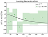 |
Fig. 7. Reconstructed lensing potential power spectrum from the polarization estimator (green points). The colored boxes denote the 1σ error regions calculated from 240 simulation sets. |
To evaluate the outcome of our lensing reconstruction, we estimated the signal-to-noise ratio (S/N) via the Fisher-matrix method,
and we used the theoretical instead of the reconstruced Cℓ in the numerator to ensure a stable prediction. ℂℓℓ′ is the covariance matrix obtained from 240 simulation sets, which reads
![$$ \begin{aligned} \mathbb{C} _{\ell \ell ^{\prime }} = \frac{1}{N-1} \sum \limits _{n=1}^{N=240} \bigg [\Big (\hat{C}^{\phi \phi }_{\ell } - \overline{C}^{\phi \phi }_{\ell }\Big )\times \Big (\hat{C}^{\phi \phi }_{\ell ^{\prime }} - \overline{C}^{\phi \phi }_{\ell ^{\prime }}\Big ) \bigg ] , \end{aligned} $$](/articles/aa/full_html/2025/02/aa52588-24/aa52588-24-eq50.gif)
where  is the averaged lensing-potential power spectrum based on the simulation sets. The final S/N obtained from the multipole range of ℓ ∈ (20, 340) is S/N ≈4.2, and this number is consistent with Han et al. (2023b), where we reported an S/N ≈4.5 with the same foreground-removing and lensing- reconstruction pipeline using a database without systematics. We therefore conclude that the systematic residual does not contaminate the lensing reconstruction strongly.
4.5. Tensor-to-scalar ratio bias
In this section, we estimate the bias on the tensor-to-scalar ratio r due to the beam systematic residual by comparing the estimated r bias of the simulations with (after deprojection) and without the beam systematics.
We sampled the posterior distribution of the tensor-to-scalar ratio r from the averaged cILC-cleaned BB power spectra by an MCMC analysis. We assumed the Gaussian likelihood of r given the cleaned band powers  as
as
![$$ \begin{aligned} \begin{aligned} - 2 \ln \mathcal{L} (r) = \sum _{\ell _b \ell _{b^{\prime }}}&\left[\hat{C}_{\ell _b} - rC_{\ell _b}^{r=1} - C_{\ell _b}^\mathrm{lens} \right]\left[M^{-1}_{\rm fid}\right]_{ \ell _b \ell _{b^{\prime }}} \\&\left[\hat{C}_{\ell _{b^{\prime }}} - rC_{\ell _{b^{\prime }}}^{r=1} - C_{\ell _b}^\mathrm{lens} \right], \end{aligned} \end{aligned} $$](/articles/aa/full_html/2025/02/aa52588-24/aa52588-24-eq53.gif)
where ℓb, ℓb′ are indices for multipole bins, rCℓbr = 1 + Cℓblens refers to the theoretical binned BB power spectrum with a multipole range of ℓ ∈ [40, 200] including 5 ℓb,  is the B-mode spectrum due to gravitational lensing,
  is the B-mode spectrum sourced by tensor perturbations with r = 1, and
 ![$ [\boldsymbol M_{\mathrm{fid}}]_{\ell_b \ell_{b{\prime}}} = \langle(\hat C_{\mathrm{fid,}\ell_b} - \langle \hat C_{\mathrm{fid,}\ell_b}\rangle) (\hat C_{\mathrm{fid,}\ell_{b{\prime}}} - \langle \hat C_{\mathrm{fid,}\ell_{b{\prime}}}\rangle)\rangle $](/articles/aa/full_html/2025/02/aa52588-24/aa52588-24-eq56.gif) is the fiducial covariance matrix computed from 300 systematics-free simulations. We derived the posterior distribution function assuming a uniform prior of r ∈ [0, 1]. We constructed an MCMC chain consisting of 10 000 samples that satisfied the posterior distribution using the emcee (Foreman-Mackey et al. 2013) Python package. We obtained the 1σ confidence interval (C.I.) and the 95% upper limit of r for the deprojection- and systematics-free cases.
is the fiducial covariance matrix computed from 300 systematics-free simulations. We derived the posterior distribution function assuming a uniform prior of r ∈ [0, 1]. We constructed an MCMC chain consisting of 10 000 samples that satisfied the posterior distribution using the emcee (Foreman-Mackey et al. 2013) Python package. We obtained the 1σ confidence interval (C.I.) and the 95% upper limit of r for the deprojection- and systematics-free cases.
The distribution of r is shown in Fig. 8. The resulting 1σ C.I. for the systematics-free case is r = 0.019 ± 0.013 and the 95% C.I. is r < 0.043, while for the deprojection case, the results are nearly the same. We note that in the selected scales ℓ ∈ [40, 200] where the B-mode spectrum is sensitive to tensor perturbations, the deprojection residual is negligible compared to the tensor power spectrum  and foreground contaminants (see Fig. 6). Therefore, the beam systematics imprint negligible effects on the measurements of r.
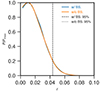 |
Fig. 8. Distribution of the tensor-to-scalar ratio for the cases with and without beam systematics. The dashed vertical lines represent the 95% upper bound, which is 0.043 for the two cases. |
5. Conclusions
We forecast the systematic effects of beam mismatches on the forthcoming S3 observations. We adopted the deprojection technique in the map-making procedure to mitigate the T → P leakage induced by the random beam mismatches added to the S3 mock TOD, and we then assessed the performance of the deprojection on the foreground cleaning, lensing reconstruction, and r-estimation. First, we compared the CMB-plus-foregrounds after deprojection and the input CMB-plus-foregrounds without instrumental effects in terms of the TEB maps and the angular power spectra. The CMB and foregrounds are mixed up in deprojection and thus cannot be separated from each other. We found that the residual leakage can be ignored compared to the input CMB-plus-foregrounds.
Then, we imposed the foreground-cleaning methods, NILC for T and E modes and cILC for B modes, on the 300 simulations of seven frequency bands including the S3 bands, the Planck HFI bands, and the WMAP K band, where the S3 mock data are deprojected. The power spectrum of the biases consisting of the residual T → P leakage and foregrounds was shown to be negligible compared to the noise uncertainties for the TT, EE, TE, or BB power. We evaluated the effect of beam systematics on the lensing reconstruction. Our lensing-potential power spectrum reconstructed from the polarization estimator has a similar signal-to-noise ratio as that obtained in previous analyses without systematics, which demonstrates that the lensing reconstruction is almost unaffected by residual systematics. Finally, we set constraints on the tensor-to-scalar ratio r using the cleaned BB spectrum, where we obtained similar results with and without beam systematics because the deprojection technique mitigates the systematics to a negligible level. Our results justify the use of a deprojection to filter the T → P leakage due to beam mismatches in S3 experiments, and the residual leakage can be ignored in the following data analysis pipeline. The effects of far sidelobes are not involved in this work since they are related to the specific shielding system of the telescope (BICEP2/Keck Collaboration 2015) and the calibration or modeling of the realistic beam maps (Gallardo et al. 2018). The undeprojected residual due to the differential beams of the sidelobes will be calibrated in future works.
If the beams of the two detectors within a pair were distorted identically, the total miscalibration effect would not induce the T → P leakage, but other systematics instead (BICEP/Keck Collaboration 2023). Several filtering systematics that may cause the E → B leakage have been discussed in Ghosh et al. (2022).
Acknowledgments
We thank Zirui Zhang, Siyu Li and Jing Jin for helpful discussions. This work is supported by the National Key R&D Program of China Grant No. 2021YFC2203102, 2020YFC2201603, NSFC No. 12325301 and 12273035. Jiakang Han thanks Stefano Camera for various support for this project. Some of the results in this paper have been derived using the pymaster, emcee, healpy, and HEALPix packages.
References
- Abazajian, K. N., Adshead, P., Ahmed, Z., et al. 2016, ArXiv e-prints [arXiv:1610.02743] [Google Scholar]
- Abazajian, K., Abdulghafour, A., Addison, G. E., et al. 2022, ArXiv e-prints [arXiv:2203.08024] [Google Scholar]
- Alonso, D., Sanchez, J., & Slosar, A. 2019, MNRAS, 484, 4127 [Google Scholar]
- Basak, S., & Delabrouille, J. 2012, MNRAS, 419, 1163 [Google Scholar]
- Basak, S., & Delabrouille, J. 2013, MNRAS, 435, 18 [Google Scholar]
- Bennett, C. L., Larson, D., Weiland, J. L., et al. 2013, ApJS, 208, 20 [Google Scholar]
- BICEP/Keck Collaboration (Ade, P. A. R., et al.) 2021, PRL, 127, 151301 [NASA ADS] [CrossRef] [Google Scholar]
- BICEP/Keck Collaboration (Ade, P. A. R., et al.) 2023, ApJ, 949, 43 [NASA ADS] [CrossRef] [Google Scholar]
- BICEP2 Collaboration (Ade, P., et al.) 2014, ApJ, 792, 62 [CrossRef] [Google Scholar]
- BICEP2 Collaboration (Ade, P. A. R., et al.) 2015, ApJ, 814, 110 [Google Scholar]
- BICEP2/Keck Collaboration (Ade, P. A. R., et al.) 2015, ApJ, 806, 206 [NASA ADS] [CrossRef] [Google Scholar]
- Blanchard, A., & Schneider, J. 1987, A&A, 184, 1 [NASA ADS] [Google Scholar]
- Carron, J., & Lewis, A. 2017, PRD, 96, 063510 [NASA ADS] [CrossRef] [Google Scholar]
- CMB-S4 Collaboration (Abazajian, K., et al.) 2022, ApJ, 926, 54 [CrossRef] [Google Scholar]
- Delabrouille, J., Cardoso, J.-F., Jeune, M. L., et al. 2009, A&A, 493, 835 [NASA ADS] [CrossRef] [EDP Sciences] [Google Scholar]
- Delabrouille, J., Betoule, M., Melin, J.-B., et al. 2013, A&A, 553, A96 [NASA ADS] [CrossRef] [EDP Sciences] [Google Scholar]
- Dou, J., Ghosh, S., Santos, L., & Zhao, W. 2024, JCAP, 05, 006 [CrossRef] [Google Scholar]
- Essinger-Hileman, T., Ali, A., Amiri, M., et al. 2014, in Millimeter, Submillimeter, and Far-Infrared Detectors and Instrumentation for Astronomy VII, eds. W. S. Holland, & J. Zmuidzinas, Int. Soc. Opt. Photon. (SPIE), 9153, 91531I [NASA ADS] [CrossRef] [Google Scholar]
- Foreman-Mackey, D., Hogg, D. W., Lang, D., & Goodman, J. 2013, Publ. Astron. Soc. Pac., 125, 306 [CrossRef] [Google Scholar]
- Gallardo, P. A., Cothard, N. F., Puddu, R., et al. 2018, in Millimeter, Submillimeter, and Far-Infrared Detectors and Instrumentation for Astronomy IX, eds. J. Zmuidzinas, & J. R. Gao, Int. Soc. Opt. Photon. (SPIE), 10708, 107082L [NASA ADS] [Google Scholar]
- Ghosh, S., Delabrouille, J., Zhao, W., & Santos, L. 2021, JCAP, 2021, 036 [CrossRef] [Google Scholar]
- Ghosh, S., Liu, Y., Zhang, L., et al. 2022, JCAP, 10, 063 [CrossRef] [Google Scholar]
- Gorski, K. M., Hivon, E., Banday, A. J., et al. 2005, ApJ, 622, 759 [Google Scholar]
- Han, J., Cao, Y., & Hu, B. 2023a, Sci. Sin. Phys. Mech. & Astron., 53, 119511 [CrossRef] [Google Scholar]
- Han, J., Hu, B., Ghosh, S., et al. 2023b, JCAP, 04, 063 [CrossRef] [Google Scholar]
- Harrington, K., Marriage, T., & Ali, A. 2016, in Millimeter, Submillimeter, and Far-Infrared Detectors and Instrumentation for Astronomy VIII, eds. W. S. Holland, & J. Zmuidzinas, Int. Soc. Opt. Photon. (SPIE), 9914, 99141K [NASA ADS] [CrossRef] [Google Scholar]
- Hazumi, M., Ade, P. A. R., Akiba, Y., et al. 2019, J. Low Temp. Phys., 194, 443 [Google Scholar]
- Hu, W. 2001, ApJ, 557, L79 [NASA ADS] [CrossRef] [Google Scholar]
- Hu, W., & Okamoto, T. 2002, ApJ, 574, 566 [CrossRef] [Google Scholar]
- Hu, W., Hedman, M. M., & Zaldarriaga, M. 2003, PRD, 67, 043004 [NASA ADS] [CrossRef] [Google Scholar]
- Kesden, M., Cooray, A., & Kamionkowski, M. 2003, PRD, 67, 123507 [NASA ADS] [CrossRef] [Google Scholar]
- Lewis, A., Challinor, A., & Lasenby, A. 2000, ApJ, 538, 473 [Google Scholar]
- Li, H., Li, S.-Y., Liu, Y., et al. 2019, Natl. Sci. Rev., 6, 145 [Google Scholar]
- Li, H., Li, S.-Y., Liu, Y., Li, Y.-P., & Zhang, X. 2018, Nat. Astron., 2, 104 [CrossRef] [Google Scholar]
- Liu, H., Creswell, J., & Dachlythra, K. 2019a, JCAP, 2019, 046 [Google Scholar]
- Liu, H., Creswell, J., von Hausegger, S., & Naselsky, P. 2019b, PRD, 100, 023538 [NASA ADS] [CrossRef] [Google Scholar]
- Liu, J., Han, J., & Hu, B. 2022a, Sci. Sin. Phys. Mech. & Astron., 52, 269811 [CrossRef] [Google Scholar]
- Liu, J., Sun, Z., Han, J., et al. 2022b, Sci. China Phys. Mech. Astron., 65, 109511 [NASA ADS] [CrossRef] [Google Scholar]
- Louis, T., Grace, E., Hasselfield, M., et al. 2017, JCAP, 06, 031 [CrossRef] [Google Scholar]
- Maniyar, A. S., Ali-Haïmoud, Y., Carron, J., Lewis, A., & Madhavacheril, M. S. 2021, PRD, 103, 083524 [NASA ADS] [CrossRef] [Google Scholar]
- Mennella, A., Ade, P., Amico, G., et al. 2019, Universe, 5, 42 [NASA ADS] [CrossRef] [Google Scholar]
- Okamoto, T., & Hu, W. 2003, PRD, 67, 083002 [NASA ADS] [CrossRef] [Google Scholar]
- Planck Collaboration IV. 2020, A&A, 641, A4 [NASA ADS] [CrossRef] [EDP Sciences] [Google Scholar]
- Planck Collaboration VI. 2020, A&A, 641, A6 [NASA ADS] [CrossRef] [EDP Sciences] [Google Scholar]
- Planck Collaboration VIII. 2020, A&A, 641, A8 [NASA ADS] [CrossRef] [EDP Sciences] [Google Scholar]
- Planck Collaboration Int. XLVIII. 2016, A&A, 596, A109 [NASA ADS] [CrossRef] [EDP Sciences] [Google Scholar]
- Planck Collaboration Int. LVII. 2020, A&A, 643, A42 [NASA ADS] [CrossRef] [EDP Sciences] [Google Scholar]
- Reinecke, M., Belkner, S., & Carron, J. 2023, A&A, 678, A165 [NASA ADS] [CrossRef] [EDP Sciences] [Google Scholar]
- Remazeilles, M., Delabrouille, J., & Cardoso, J.-F. 2011, MNRAS, 410, 2481 [Google Scholar]
- Remazeilles, M., Rotti, A., & Chluba, J. 2021, MNRAS, 503, 2478 [NASA ADS] [CrossRef] [Google Scholar]
- Sayre, J. T., Reichardt, C. L., Henning, J. W., et al. 2020, PRD, 101, 122003 [NASA ADS] [CrossRef] [Google Scholar]
- Sheehy, C. 2019, arXiv e-prints [arXiv:1911.03547] [Google Scholar]
- Simons Observatory Collaboration (Ade, P., et al.) 2019, JCAP, 2019, 056 [CrossRef] [Google Scholar]
- Tristram, M., Banday, A. J., Górski, K. M., et al. 2022, PRD, 105, 083524 [NASA ADS] [CrossRef] [Google Scholar]
- Zaldarriaga, M., & Seljak, U. 1998, PRD, 58, 023003 [NASA ADS] [CrossRef] [Google Scholar]
- Zhao, W., & Baskaran, D. 2010, PRD, 82, 023001 [NASA ADS] [CrossRef] [Google Scholar]
- Zonca, A., Singer, L., Lenz, D., et al. 2019, JOSS, 4, 1298 [NASA ADS] [CrossRef] [Google Scholar]
Appendix A: Recovered beam parameters versus the input ones
Figure A.1 shows the comparison between the fitted beam mismatch parameters in deprojection and the input values for 1728 detector pairs of a realization at 150 GHz. The red solid curves refer to y = x, and the red dashed curve was vertically offset by the estimated mean bias on δp (7.2 × 10⁻³). The Pearson correlation coefficient R approaching 1 for all parameters indicates a strong correlation between the deprojection coefficients and the input parameters, demonstrating the precision of deprojection. The standard deviation of the bias (Δ) on each coefficient is significantly lower than the median measurement uncertainty for individual detectors by BICEP2/Keck Array (see BICEP2/Keck Collaboration 2015, Table 3), but is too optimistic since the noise was not added to the data.
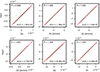 |
Fig. A.1. Scatter plot of the recovered beam mismatch parameters averaged over time trunks (x-axis) vs. the input values (y-axis) for all 1728 detector pairs of a simulation at 150 GHz. The red solid curves have a slope of 1 and a y-intercept of 0. The red dashed curve has been offset vertically by the mean bias on δp estimated from systematics-free simulations. The correlation coefficient R and the standard deviation of the bias on the deprojection coefficient σ(Δ) are exhibited. |
Appendix B: PCL-TC estimator
The E → B mixing is introduced when the partial-sky Q and U maps are converted to the E and B modes in harmonic space (Zhao & Baskaran 2010; Ghosh et al. 2021). We used the template cleaning method (Liu et al. 2019a,b) to get rid of the resulting E → B leakage. To estimate the full-sky B-mode power spectrum from foreground-cleaned maps, we adopted the pseudo-Cℓ method to account for mode-coupling induced by masking and multipole binning using the NaMASTER (Alonso et al. 2019)6 package. The whole process is called the “PCL-TC” estimation.
The template cleaning method is a pixel-based technique to remove E → B leakage due to partial-sky effects. The steps are as follows:
-
First convert the masked (Q, U) maps into (aℓmE, aℓmB) using the map2alm function of healpy (Zonca et al. 2019). Transform aℓmB into the B map being contaminated by the E → B leakage, Bc.
-
Convert the E-only modes (aℓmE, 0) back into maps (QE, UE) using the alm2map function of healpy. Multiply them by the mask and convert them into
 using map2alm. The B map derived from
  is taken as our E → B leakage template, Bt.
 -
Linearly fit the masked leakage template Bt to the masked contaminated map Bc in the pixel space. Finally subtract the fitted leakage to obtain the pure B-mode map:
 where α is the linear coefficient.
Deprojection, as any other filtering operation on Q and U time streams, can produce a small amount of E → B mixing. The E → B leakage due to deprojection can also be corrected for by taking advantage of the deprojected E-mode only data to get a B-mode leakage template (see Ghosh et al. 2022, Sect. 4.2).
After the foreground cleaning, we corrected for the common beam (11 arcmin) and pixel window functions in the aℓm’s. Finally we computed the full-sky bandpowers with a bin size of 30 using the decouple_cell module of pymaster.
All Tables
Six beam mismatch parameters added to the mock TOD and the corresponding leakage templates.
All Figures
|
Fig. 1. Distribution of the recovered beam mismatch parameters of 106 time trunks for one detector pair of a noise-free simulation at 150 GHz. The dashed red lines represent the input beam parameter, and the dashed black lines indicate the mean over all time series. There is a bias on the differential plus-ellipticity of Δ ≈ 7.3 × 10⁻³ due to the cosmological TE correlation. |
| In the text | |
|
Fig. 2. Maps of CMB plus foregrounds at S3 150 GHz. First row: Input B-mode CMB and foregrounds without beam systematics (left), CMB plus foregrounds with beam systematics (middle) and after deprojection (right). Second row: Difference between the deprojected map and the input map without beam systematics for the T (left), E (middle), and B (right) modes. The results of 95 GHz are similar to the 150 GHz results. |
| In the text | |
|
Fig. 3. TT, EE, TE, and BB power spectra of the 150 GHz CMB plus foregrounds map with beam systematics before (blue curves) and after deprojection (red curves) for one realization. The input CMB+FG. power spectrum without beam systematics is shown as a solid black curve for comparison with the deprojected one, and their difference, the residual after deprojection, is shown as a dashed cyan curve. The results of 95 GHz are similar to the 150 GHz results. |
| In the text | |
|
Fig. 4. Maps of the input CMB (left column), the foreground-cleaned maps (middle column), and their difference, i.e., the residual maps (right column) for the T, E, and B modes. The first row shows T maps, the second row shows E maps, and the third row shows B maps. |
| In the text | |
|
Fig. 5. cILC residual B maps of the systematics (left), foreground (middle), and noise (right) components for one realization. |
| In the text | |
|
Fig. 6. Power spectra including NILC-cleaned TT (left top), NILC-cleaned EE (right top), NILC-cleaned TE (left bottom), and cILC-cleaned BB (right bottom) power spectra with ℓmax = 1500. The input CMB (solid black curves), the reconstructed CMB (blue bars), and the residual noise (orange curves) power spectra are plotted in each panel. The green curves represent the sum of the systematic and foreground residuals. For the BB spectra, the deprojection and foreground residuals are separately shown as red and purple curves, respectively. The power spectra are binned over every 30 multipoles except for the BB spectra, where a logarithm binning at ℓ > 100 was adopted for clarity. |
| In the text | |
|
Fig. 7. Reconstructed lensing potential power spectrum from the polarization estimator (green points). The colored boxes denote the 1σ error regions calculated from 240 simulation sets. |
| In the text | |
|
Fig. 8. Distribution of the tensor-to-scalar ratio for the cases with and without beam systematics. The dashed vertical lines represent the 95% upper bound, which is 0.043 for the two cases. |
| In the text | |
|
Fig. A.1. Scatter plot of the recovered beam mismatch parameters averaged over time trunks (x-axis) vs. the input values (y-axis) for all 1728 detector pairs of a simulation at 150 GHz. The red solid curves have a slope of 1 and a y-intercept of 0. The red dashed curve has been offset vertically by the mean bias on δp estimated from systematics-free simulations. The correlation coefficient R and the standard deviation of the bias on the deprojection coefficient σ(Δ) are exhibited. |
| In the text | |
Current usage metrics show cumulative count of Article Views (full-text article views including HTML views, PDF and ePub downloads, according to the available data) and Abstracts Views on Vision4Press platform.
Data correspond to usage on the plateform after 2015. The current usage metrics is available 48-96 hours after online publication and is updated daily on week days.
Initial download of the metrics may take a while.