| Issue |
A&A
Volume 617, September 2018
|
|
|---|---|---|
| Article Number | A96 | |
| Number of page(s) | 13 | |
| Section | Cosmology (including clusters of galaxies) | |
| DOI | https://doi.org/10.1051/0004-6361/201833288 | |
| Published online | 27 September 2018 | |
Cosmic microwave background constraints in light of priors over reionization histories
1
Institut Lagrange de Paris (ILP), Sorbonne Universités, 98bis boulevard Arago, 75014
Paris, France
e-mail: This email address is being protected from spambots. You need JavaScript enabled to view it.
2
Institut d’Astrophysique de Paris (IAP), UMR7095, CNRS & Sorbonne Universités, 98bis boulevard Arago, 75014
Paris, France
Received:
24
April
2018
Accepted:
24
May
2018
Abstract
Non-parametric reconstruction or marginalization over the history of reionization using cosmic microwave background data necessarily assumes a prior over possible histories. We show that different but reasonable choices of priors can shift current and future constraints on the reionization optical depth, τ, or correlated parameters such as the neutrino mass sum, Σmν, at the level of 0.3–0.4 σ, meaning that this analysis is somewhat prior dependent. We point out some prior-related problems with the commonly used principal component reconstruction, concluding that the significance of some recent hints of early reionization in Planck 2015 data has been overestimated. We also present the first non-parametric reconstruction applied to newer Planck intermediate (2016) data and find that the hints of early reionization disappear entirely in this more precise dataset. These results limit possible explanations of the EDGES 21cm signal which would have also significantly reionized the universe at z > 15. Our findings about the dependence on priors motivate the pursuit of improved data or searches for physical reionization models which can reduce the prior volume. The discussion here of priors is of general applicability to other non-parametric reconstructions, for example of the primordial power spectrum, of the recombination history, or of the expansion rate.
Key words: cosmic background radiation / dark ages / reionization / first stars / cosmological parameters
© ESO 2018
 Open Access article, published by EDP Sciences, under the terms of the Creative Commons Attribution License (http://creativecommons.org/licenses/by/4.0), which permits unrestricted use, distribution, and reproduction in any medium, provided the original work is properly cited.
1. Introduction
The exact details of the epoch of reionization, during which the universe transitioned from a mostly neutral hydrogen gas into the highly ionized state we see today, are still of considerable uncertainty. This transition left several imprints on the cosmic microwave background (CMB) which can be used to constrain the physics of reionization, but also serve as a “nuisance” uncertainty which must be marginalized over when considering constraints on other parameters.
One of the most widely used methods for reconstructing or marginalizing over the reionization history from CMB data has been based on decomposing the history into a set of principal component amplitudes (PCAs), described initially by Hu & Holder (2003; hereafter HH03). This has been applied to a number of datasets, for example the WMAP data (Mortonson & Hu 2008b; Pandolfi et al. 2011, the former hereafter MH08), and most recently the Planck 2015 data (Heinrich et al. 2017; Heinrich & Hu 2018; Obied et al. 2018). The latter works argue that the generic reconstruction reveals a > 2σ preference for a high-redshift (z ≳ 15) contribution to the optical depth, τ. Other works have used alternate methods, some finding somewhat similar preference for a high-redshift contribution (Hazra & Smoot 2017), while others finding none at all (Villanueva-Domingo et al. 2018).
In this work, we point out two problems with PCA analyses that have to-date been largely or completely overlooked. Correcting these problems will lead to finding reduced evidence of early reionization in the Planck 2015 data.
The first problem has been mentioned in Mortonson & Hu (2008b), Heinrich & Hu (2018), and described in some detail in Lewis et al. (2006), although not explicitly in relation to the PCA model. The issue is that taking a flat prior on amplitudes of the reionization principal components induces a non-flat prior on τ. Heinrich & Hu (2018) argue that this effect is unimportant, but do not perform direct or fully conclusive tests. Here we have performed the very direct test of simply calculating the effective τ prior induced by the flat mode priors, finding that it is roughly τ ≈ 0.20 ± 0.07. Using a maximum entropy procedure, we remove the effects of this prior, finding that it accounts for a significant part of the shift to higher τ reported by Heinrich et al. (2017).
Another problem with existing PCA analyses lies in the choice of physicality priors. These priors are necessary to ensure that the reconstructed ionization fraction at any given redshift remains within physical range (i.e. remains positive but less that the maximum corresponding to a fully ionized universe). Due to the nature of the PCA decomposition, the standard physicality priors necessarily allow some unphysical models (this may seem quite counter-intuitive, but we will give a simple geometric picture of why this is indeed the case). However, existing analyses have used a sub-optimal set of physicality priors which allowed more unphysical models than necessary. We will derive the optimal set of priors, and show that switching to these leads to significant changes in constraints. Together with removing the impact of the informative τ prior, we find that evidence for early reionization in the Planck 2015 data is reduced from > 2σ to 1.4σ.
Since the PCA results depend significantly on the details of the physicality priors, which will always be necessarily imperfect, we conclude that the PCA procedure is poorly tailored to the problem of generic reionization history reconstruction. We seek a better method, in particular one which does not allow unphysical models. To this end, we propose what we will call the FlexKnot model. This model interpolates the history using a varying number of knots, with the exact number of knots determined by the data itself via a Bayesian evidence calculation. The model is somewhat similar to the Hazra & Smoot (2017) approach, but improves upon it by not requiring an a posteriori and fixed choice of knot positions, which otherwise creates undesired regions of high prior probability at certain redshifts. The FlexKnot model follows almost exactly the same procedure used previously to generically reconstruct the primordial power spectrum from Planck data (Vázquez et al. 2012; Planck Collaboration XX 2016), and is particularly well suited to the problem here as well.
Using these reionization models, we calculate new constraints on the history of reionization coming from Planck intermediate data, in particular using the simlow likelihood (Planck Collaboration Int. XLVI 2016). We will refer to the combination of Planck 2015 data and the simlow likelihood as the Planck 2016 data. This likelihood has already been used to explore various parametric reionization models (Planck Collaboration Int. XLVII 2016); however, a generic reconstruction fully capable of detecting an early component to reionization (should it be there) has not yet been performed. We report results from this particular dataset here.
The Planck 2016 data represents a significant increase in constraining power on reionization as compared to the 2015 data, and we find that the remaining 1.4σ hints of an early reionization component are completely erased. Instead, we tightly constrain the z > 15 contribution to the optical depth to be < 0.015 at 95% confidence, and find good agreement with a late and fast transition to a fully ionized universe, consistent with the conclusions of Planck Collaboration Int. XLVII (2016).
Even though the simlow data are quite constraining, some dependence on priors remains when performing generic reconstruction. In particular, the difference between a flat prior on τ and a flat prior on the knot positions leads to an 0.4σ shift in the resulting τ constraint. Both of these priors are fairly reasonable, and we consider it difficult to argue very strongly for one or the either of these priors in a completely generic setting. We thus consider this indicative of a level of systematic uncertainty stemming from our imperfect knowledge of the model, which we then propagate into shifts on other parameters which are correlated with τ, given both current data and future forecasts.
We specifically focus on the sum of the neutrino masses, Σmν, which is expected to be measured extremely precisely by next generation CMB experiments (Abazajian et al. 2015). Using Fisher forecasts, we show that a possible 0.4σ bias on τ from switching priors manifests itself as a 0.3σ bias on Σmν given expect constraints from a Stage 4 CMB experiment (CMB-S4; Abazajian et al. 2016). We comment on the ability of combining with other probes, such as DESI-BAO, or a cosmic-variance-limited CMB large-scale polarization measurement, to reduce this uncertainty.
Given these biases, we conclude that generic reconstructions of the reionization history are likely not enough to achieve the most accurate bounds on Σmν. This motivates work on obtaining constraints with physical models which have free parameters that can realistically account for our lack of exact knowledge about the physics of reionization. Although not directly used throughout the paper, will also comment on the possibility for other probes of reionization to reduce the dependence on priors, specifically measurements of the patchy kinetic Sunyaev-Zeldovich effect (Gruzinov & Hu 1998; Knox et al. 1998) and direct probes of the ionization state of the inter-galactic medium (Bouwens et al. 2015).
The paper is outlined as follows. In Sect. 2 we discuss the reionization models we consider, and in Sect. 3 we focus on the implicit τ prior induced by these procedures. These sections are a fairly technical description of the methodology used, and those wishing to see the results should skip to Sects. 4–6 where we discuss constraints from Planck 2015, intermediate, and future data, respectively.
2. Reionization models
2.1. TANH model
The reionization history often assumed in CMB analyses because it has a useful parametric form and matches physical expectations somewhat well involves a single smooth step from an almost fully neutral universe1 to one with hydrogen fully ionized and helium singly ionized. The free electron fraction, in our convention the ratio between the number density of free electrons and hydrogen nuclei, xe ≡ ne/nH, is taken to be ![Mathematical equation: $ \begin{aligned} x_\mathrm{e}^\mathrm{TANH}(z) \,{=}\, \frac{1+f_\mathrm{He}}{2}\left\{ 1+\tanh \left[\frac{y(z^*) - y(z)}{\Delta y}\right]\right\} , \end{aligned} $](/articles/aa/full_html/2018/09/aa33288-18/aa33288-18-eq1.gif) (1)
(1)
with y(z) = (1 + z)3/2 and Δy = 3/2(1 + z)1/2Δz, giving a transition centered at redshift z* with width Δz = 0.5. Here the factor fHe is the number density ratio of helium to hydrogen nuclei (we have neglected all other atoms). We will refer to this model as the TANH model.
The contribution to the optical depth between any two redshifts z1 and z2 for this (or any) reionization history can be written as (2)
(2)
where σT is the Thompson scattering cross-section. This is often used to parametrize Eq. (1) in terms of the total optical depth τ ≡ τ(0, zearly) rather than z* (where zearly is some redshift before reionization began, but after recombination ended).
Note that in this convention for xe, the maximum ionization fraction can be greater than one, in particular can be as large as  before the second recombination of helium. We also note that second helium recombination is expected to be a small contribution to τ, on the order of ≈0.001 depending on the exact values of other cosmological parameters. As this is already fairly small, we ignore any model-dependence in helium second reionization and model it as another transition with the same hyperbolic tangent form as in Eq. (1) but with z* = 3.5 and Δz = 0.5, normalized such that it increases the ionization fraction from
  to 1 + 2fHe.
2.2. PCA model
The TANH model has some parametric freedom, more-so if Δz is also taken as a free parameter. However, we would like a model which can reproduce any arbitrary history, thus allowing us to generically reconstruct xe(z) from the data.
HH03 proposes a model based on decomposing the free electron fraction history into eigenmodes such that (3)
(3)
for some fiducial  , eigenmode amplitudes mi, and eigenmode templates Si(z). These templates have support between some zmin and zmax and are uniquely defined by three properties:
-
1.
they form a special orthonormal basis2 for xe(z), implying that ∫dz Si(z)Sj(z) = δij.
-
2.
they diagonalize the covariance of the amplitude parameters given cosmic-variance-limited large-scale polarization data,
 ;
; -
3.
they are ordered by increasing σi.
2.3. Geometric view of physicality priors
The HH03 procedure also calls for a set of “physicality priors” on these mode amplitudes. These are necessary because otherwise nothing prevents the mode amplitudes from taking on values such that the bound  fails to hold for some z, and this would have no physical meaning. Mortonson & Hu (2008a) derive two sets of priors to enforce physicality. The first is an upper and lower bound on each mi such that
  with
with![Mathematical equation: $ \begin{aligned} m_i^{\pm } = \int \text{ d}z \left\{ S_i(z)\left[1-2x_\mathrm{e}^\mathrm{fid}(z)\right] \pm |S_i(z) | \right\} /2. \end{aligned} $](/articles/aa/full_html/2018/09/aa33288-18/aa33288-18-eq10.gif) (4)
(4)
The second is an upper bound on the sum of the squares of the mode amplitudes,![Mathematical equation: $ \begin{aligned} \int \text{ d}z \sum _i m_i^2 \,{<}\, \int \text{ d}z \, \big [x_\mathrm{e}^\mathrm{max} - x_\mathrm{e}^\mathrm{fid}(z)\big ]^2. \end{aligned} $](/articles/aa/full_html/2018/09/aa33288-18/aa33288-18-eq11.gif) (5)
(5)
These priors may seem a bit abstruse, but they have a quite simple geometric interpretation which has not been highlighted before. We will give this interpretation here, aided by Fig. 1. This will also aid in spotting some improvements that can be made.
To start, consider the reionization history, xe(z), evaluated at N redshifts, zi, and stacked into a vector xi ≡ xe(zi). The physicality region in the xi vector space is trivial, each xi must individually fall between 0 and  . This region is thus an N-dimensional hypercube with one vertex at the origin, extending into the positive hyper-quadrant, and with edge length
  .
.
The decomposition into mode amplitudes is given by applying the transformation S to the residual between xi and the fiducial model, (6)
(6)
where Sij ≡ Si(zj), i.e. it is a matrix for which each row is one of the eigenmodes. The physicality region in the mi vector space is thus a translated and transformed version of the original hypercube. We note that because S is special orthonormal and thus can only contain rotations, the region remains a hypercube.
Let us now visualize this transformation in two dimensions, represented in the left panel of Fig. 1. The solid blue square is the physicality region in terms of xi, here just x1 and x2. The solid orange square is the same region after transformation by Eq. (6), assuming some arbitrary S for demonstration purposes, and taking  following Mortonson & Hu (2008a) and all other subsequent PCA analyses.
If we were simultaneously fitting m1 and m2 in our analysis, the physicality region would be trivial to enforce, and would be given simply by the solid orange square. However, the point of the PCA procedure is that we do not need to simultaneously fit both parameters, as higher order modes like m2 can be effectively marginalized over by just fixing them, since they have no observable impact and are decorrelated with the lower order modes like m1. Usually we fix m2 = 0, but any other value should work just as well. In designing the physicality prior for m1, we need to ensure that all values that m1 could take are allowed, not just those allowed when m2 = 0, since this was just an artificial method of marginalization3. Put another way, one must consider that a model which appears to be unphysical could be brought back into physicality by adjusting the higher order mode amplitudes which were artificially set to zero. This leads to two priors which can be constructed.
The first prior is simply the bounding box of the solid orange square and is depicted as the dashed orange square. We refer to this as the “hyperbox” prior4. This prior just takes a hard bound on each mi corresponding to the largest and smallest possible value for that mi anywhere within the physicality region. This is indeed exactly what is calculated by Eq. (4). One can see this by noting that the xj which maximizes mi in Eq. (6) is such that  if Sij is positive, and zero otherwise, and that Eq. (4) is the transform of this xj.
The second prior comes from noting that as long as  , the top right corner of the physicality region in terms of x (i.e., the top right corner of the solid blue square in Fig. 1), will always be the furthest point from the origin even after transformation. Its distance from the origin will be unaffected by the rotation S, only by the translation by xfid, thus we can exclude points further than
  in the mode parameter space. This leads to the physicality region depicted by the dashed circle, and we will refer to this as the “hypersphere” prior. One can recognize this as the second MH08 prior in Eq. (5) by noting that integral over z there is analogous to the sum that appears in the vector norm,
  .
.
The intersection of these two priors is shaded orange, and corresponds to the full MH08 physicality region. Note that although the two priors do remove some of the allowed unphysical regions of parameter space, they can never remove all of them. As we will see in Sect. 5, this unavoidably allowed unphysical region has undesirable consequences.
While the amount of unphysical parameter space allowed by the hyperbox prior does not depend on our choice of xfid, this is not the case for the hypersphere prior. Indeed, the geometric picture makes it clear that we could reduce the allowed unphysical regions by picking xfid = xmax/2, i.e., placing the fiducial model at the center of the original hypercube5. This is depicted in the right panel of Fig. 1. This choice is optimal in the sense that no other choice of xfid excludes as much of the unphysical region, given the two priors we have constructed. As we will see in Sect. 3, using the optimal physicality region is also useful because the increased symmetries in this case allow an analytic calculation of the induced τ prior.
The physicality prior obtained by taking xfid to be in the center of the physicality region is objectively better than other choices, and should be used. It does not bias the analysis in any other way, in fact it prevents biases from an over-allowance of unphysical parameters. We will show in Sects. 4 and 5 that the “sub-optimality” of the MH08 prior has a significant impact on constraints from data.
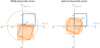 |
Fig. 1. Geometric picture of the PCA physicality priors in two-dimensions, demonstrating why they necessarily allow unphysical regions of parameter space. The solid blue square is the physicality region in terms of the ionization fraction, x1 and x2, at individual redshifts. The solid orange square is the physicality region in terms of the mode amplitudes, m1 and m2. The two types of physicality priors corresponding to Eq. (4) and Eq. (5) are shown as the dashed square and dashed circle, respectively. Their intersection, shaded orange, is the full physicality region. The left panel takes a fiducial ionization history, xfid = 0.15, consistent with Mortonson & Hu (2008a) and subsequent works. The right panel shows that the undesired but allowed unphysical parameter space can be reduced (but not fully) with a better choice of fiducial model. |
2.4. HS17 model
As discussed in the previous section and elsewhere (e.g. Mortonson & Hu 2008a), one draw-back of the PCA model is the necessary inclusion of unphysical parameter space in the prior. In some sense this is because the PCA procedure rotates the parameters from a space in which the prior is easy to describe to one in which the likelihood is easy to describe. If we are in a regime where the prior is completely uninformative, this is a very beneficial rotation; here, however, this is not quite the case.
One solution is thus to not perform the PCA rotation at all, and keep the values of ionization fraction at some given redshifts (the xi) as the parameters. Then we can always fully and sufficiently enforce physicality by requiring that  for all z. Variations on this avenue have been explored, for example, by Colombo & Pierpaoli (2009), Lewis et al. (2006), and Hazra & Smoot (2017). In this section we consider for definiteness the latter model, which we denote the HS17 model.
The HS17 model takes uniform priors on the values of xe(z) at z = 6, 7.5, 10, and 20, with end-points at  and xe(30) = 0 fixed, and interpolates everywhere in between these knots using piecewise cubic Hermite interpolating polynomials (PCHIP). Although the choice is ad-hoc and made somewhat a posteriori (which makes judging the statistical evidence for this model difficult), it does likely capture much of the observable features of the reionization history. A larger problem, however, is that it creates an undesired prior distribution, shown in the middle panel of Fig. 2. While the prior on xe(z) at the z-values of the knots is uniform, it becomes triangular at the mid-point between knots, leading to the odd patterns seen in this figure. With a simple modification of this model, which we give in the next section, we are able to remove this oddly patterned prior.
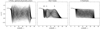 |
Fig. 2. One thousand reionization histories sampled from their prior distribution given the different models we consider. In the PCA case, the prior over PCA modes is taken to be uniform within the physicality region; in the two knot cases, the prior is uniform on the position and/or amplitude of each knot (thus none of these priors correspond to a flat τ priors). The left panel shows the extent to which the PCA procedure allows unphysical models, even when using the optimal physicality priors. The middle panel shows that the HS17 prior creates odd features and tighter peaked priors in the regions between the knot locations (which are indicated with arrows). The right panel is the prior for the FlexKnot model and represents our best solution for creating a reasonable and “homogeneous” prior. |
2.5. FlexKnots
To remedy the non-idealities of both the PCA and HS17 models discussed thus-far, we develop the following model and analysis procedure, inspired by the primordial power spectrum reconstruction in the Planck analysis (Vázquez et al. 2012; Planck Collaboration XX 2016).
The model, which we call the FlexKnot model, has knots which can move left and right in addition to up and down. Our parameters are thus a set of xi and zi, with uniform priors across the ranges (7)
(7)
 (8)
(8)
Additionally, given any set of zi, we compute the reionization history by first sorting them before interpolating between the knots (see also Appendix A2 of Handley et al. 2015b). We perform interpolation using the PCHIP scheme, similarly as to what is done in HS17.
Samples from this prior with 5 knots are shown in the right-most panel of Fig. 2. We see that the prior distribution is much more uniform than the HS17 prior, with no clustering around any particular redshift or ionization fraction value. This is the effect of the left/right freedom of knots, coupled with the sorting procedure.
A final question for the FlexKnot model remains, mainly how many knots to allow? We follow Planck Collaboration XX (2016) in marginalizing over the number of knots by computing the Bayesian evidence for each of n knots, (9)
(9)
where ℒn and 𝒫n are the likelihood and prior given n, and computing the posterior distribution marginalized over n, (10)
(10)
Here, y can represent the ionization fraction history, τ, or any other derived quantity of interest. The πn are the prior weights which we give to a model with n knots; we set this equal to one, i.e, we assume that every number of knots is equally probable. The evidence computation is performed in practice with POLYCHORD (Handley et al. 2015a; Handley et al. 2015b).
Given the necessity of choosing the πn, one should ask: have we really gained anything by this procedure, or have we just swapped the requirement of making one choice of prior for another? To answer this, note that although some choice still remains, we have reduced the problem of picking a functional prior over all possible histories to one of simply picking a prior over which integer number of knots to take. This is a massive reduction in how arbitrary a choice we are required to make, and represents the key strength of this procedure. Additionally, as we will show in the next section, the data themselves largely disfavor the need for anything beyond one or two knots anyways, thus we are not particularly sensitive to the πn, as long as a reasonable choice is made.
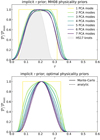 |
Fig. 3. Solid colored lines: implicit prior on τ from the PCA model when taking a flat prior on the mode amplitudes, computed via Monte Carlo. The top panel assumes the MH08 physicality region, whereas the bottom panel assumes our optimal physicality region. In the case of the bottom panel, analytic calculation of the prior is possible via Eq. (15) and shown as dotted lines. The top panel also shows the implicit prior for the HS17 model. |
3. Implicit prior on τ
3.1. Calculating the prior
Although the details of how reionization proceeds are of significant physical interest, it is mostly the total overall integrated optical depth to reionization, τ, that plays an important role in terms of CMB constraints. This is because τ modulates the amplitude of temperature and polarization power spectra at multipoles greater that a few tens by e−2τ, and is thus a source of degeneracy for the scalar amplitude, As, which does the same. The parameter As itself is then degenerate with a number of other physical quantities of interest via various means (Planck Collaboration Int. LI 2017). It is thus important to examine what these different methods of reconstruction have to say in terms of τ.
In particular, what prior over τ do the different approaches assume? Take, for example, the PCA model. Because the modes contribute linearly to xe(z) and because τ is in turn a linear functional of xe(z), each mode contributes linearly to the total optical depth, (11)
(11)
where τfid is the optical depth corresponding to  and
and (12)
(12)
In all analyses to-date, the prior taken on the mi has been uniform inside of the physicality region. We can compute the τ prior induced by this choice by propagating the mi prior to τ via Eq. (11). If the mi are uncorrelated in the prior (which is a decent approximation if using the MH08 physicality priors where the hypersphere prior plays a sub-dominant role) the induced τ prior will be a convolution of a number of “top-hat” functions, which should tends toward some smooth distribution. The exact solution (including both hyperbox and hypersphere) can be obtained numerically by Monte Carlo sampling from the mi prior and computing τ for each sample. This is shown in the top panel of Fig. 3. Indeed, we find that the prior is centered on τ ≈ 0.2 and has width around σ(τ) ≈ 0.07, tightening and smoothing out as more modes are added. The mean prior value of τ ≈ 0.2 is the optical depth corresponding to an ionization level of  throughout the entire z = [6, 30] reconstruction region, as this is what is given by the mean mode values,
  , independent of fiducial model (here ignoring the hypersphere prior, which is a good approximation in terms of the mode mean).
It is important to note the existence of this prior when comparing constraints on τ from two different models, for example the TANH model (which takes a flat τ prior) and the PCA model. In such comparisons, we change not only the model but also implicitly change the prior. Given that the prior we see in Fig. 3 tends toward quite high values of τ, it should not be entirely surprising if we find a higher τ posterior in the PCA case. In Sect. 4 we will quantify the impact this has on the Heinrich et al. (2017) analysis.
What about the induced prior in the case of the optimal physicality prior instead of the MH08 one? Here, the extra symmetries of the problem allow us to derive the following useful analytic solution. First, consider the simplified case of computing the τ prior induced by only the hypersphere prior. This is given by![Mathematical equation: $ \begin{aligned} \mathcal P (\tau ) \,{=}\, \int _\mathbb{S }\; \displaystyle \prod _{i\,{=}\,1}^{N} \text{ d}m_i \;\delta \left[\tau - \tau \big (\{m_i\}\big )\right], \end{aligned} $](/articles/aa/full_html/2018/09/aa33288-18/aa33288-18-eq31.gif) (13)
(13)
where the region 𝕊 is an N-dimensional hypersphere with radius  and centered on the origin, and δ is the Dirac δ-function. In geometric terms, Eq. (13) calculates the volume of the intersection of the hyperplane defined by τ − τ({mi}) = 0 with the hypersphere 𝕊. This intersection is itself an N − 1 dimensional hypersphere. Its radius, ρ, is smaller than r due the hyperplane having sliced through 𝕊 at a position displaced from its center. The displacement distance is controlled by τ and given by D = |τ − τfid|/|g|, where we have defined a vector normal to the hyperplane, (g)i ≡ dτ/dmi. This allows us to compute the smaller radius, ρ2 = r2 − D2, and, using the formula for the volume of a hypersphere, we arrive at the final answer,
![Mathematical equation: $ \begin{aligned} \mathcal P (\tau ) \propto \frac{\pi ^{\frac{N-1}{2}}}{\Gamma \bigg (\frac{N}{2}-1\bigg )} \rho ^{N-1} \propto \left[1-\frac{(\tau -\tau _\mathrm{fid})^2}{r^2|\mathbf{g}|^2}\right]^{\frac{N-1}{2}}. \end{aligned} $](/articles/aa/full_html/2018/09/aa33288-18/aa33288-18-eq33.gif) (14)
(14)
Note that, as written, neither of these forms are a properly normalized probability distribution (however, this is not a requirement for our purposes, and the proper normalization is straightforward to compute if desired).
We now need to include the fact that the hyperbox prior excludes some of the hypersphere prior, as represented in two dimensions in the right panel of Fig. 1. In general, this breaks the symmetries which made Eq. (14) so simple. We find, however, that because dτ/dm1 is much larger than any of the other derivatives, it is predominantly only the exclusion in the m1 direction which needs to be accounted for. This leaves enough symmetry that the resulting solution is simple enough to be useful.
The above calculation needs to be amended in the following way. Define 𝕊′ to be intersection of the hypersphere with the region defined by  ; i.e., 𝕊′ is a hypersphere with two opposite hyper-spherical caps removed. As τ is increased or decreased from τfid, changing where the hyperplane intersects with 𝕊′, the intersection region initially does not also intersect with the caps, leaving the solution unchanged from before. Once it does intersect with the caps, the intersection region is now no longer an N − 1 dimensional hypersphere, but rather an N − 1 dimensional hypersphere with a single hyper-spherical cap removed. Thus, the induced prior will be instead
 (15)
(15)
where V is the volume of the removed hyper-spherical cap relative to the volume of the entire hypersphere. This fraction can be written in terms of the regularized incomplete beta function, Ix(a, b) (Li 2011), and is given by (16)
(16)
where h is the height of the cap, h = ρ − m( + ) csc θ + Dcot θ, and θ is the angle between the hyperplane and the m̂1 direction, cos θ = g1/|g|.
The bottom panel of Fig. 3 shows this analytic result for several values of N, alongside the Monte Carlo calculation performed similarly as before. The “kink” near τ ∼ 0.1 (visible particularly in the N = 2 curve, although present in all of them) corresponds to when the correction, V, turns on; without this, we would not recover the correct shape in the tails of the distribution. With it, however, we find very good agreement between the Monte Carlo simulations and the analytic result, particularly deep in the low-τ tail which is most important since this is the region picked out by the data. This analytic result will be useful in the next section where we discuss flattening the prior. Note also that the prior volume for τ shrinks noticeably as compared to the MH08 physicality region; we will show in Sect. 4 that this smaller and more optimal prior volume is enough to affect constraints from Planck data.
Similarly as to the PCA model, both the HS17 knot model and our FlexKnot model give a non-flat τ prior if the prior on the knot amplitudes and/or positions is taken as flat. The prior for the HS17 model is shown in the top panel of Fig. 3. The FlexKnot prior is not shown, but is qualitatively similar to the others.
3.2. Flattening the prior
Having ascertained that all of the generic reconstruction methods we have discussed implicitly place a non-flat prior on τ, we now discuss how to modify these analyses so that any desired τ prior can be used, in particular a uniform one. This will be useful in performing more consistent comparisons between models by using the same prior on τ for all models.
Intuitively, if we have an MCMC chain for an analysis that was performed with some particular τ prior, we can importance sample the chain to give additional weight to samples with a low prior probability for τ, in effect counter-balancing the original prior and forcing it to be flat. More explicitly, we can create a posterior where we have assumed a flat τ prior by computing![Mathematical equation: ${{\mathcal{P}}^{\text{flat}-\tau }}(\theta |d)=\frac{{{\mathcal{P}}^{\text{orig}}}(\theta |d)}{{{\mathcal{P}}^{\text{orig}}}(\tau (\theta ))}\propto \mathcal{L}(d|\theta )\underbrace{\left[ \frac{{{\mathcal{P}}^{\text{orig}}}(\theta )}{{{\mathcal{P}}^{\text{orig}}}(\tau (\theta ))} \right]}_{{{\mathcal{P}}^{\text{flat}-\tau }}(\theta )}, $](/articles/aa/full_html/2018/09/aa33288-18/aa33288-18-eq37.gif) (17)
(17)
where the posterior 𝒫orig(θ | d) given data d is the original posterior that did not assume a flat τ prior, 𝒫orig(θ) and 𝒫orig(τ(θ)) are the original priors in terms of all parameters θ and the induced τ prior, respectively, and ℒ(d | θ) is the likelihood of the data given parameters. In the case of the PCA model with optimal physicality priors, 𝒫orig(τ(θ)) is conveniently calculable analytically and given in Eq. (15). For other models, it can be obtained via Monte Carlo simulations and a smooth function can be fit (e.g. here we use kernel density estimates with tools from Lewis & Xu 2016).
We should note that this procedure is not unique, and many 𝒫flat-τ(θ) exist corresponding to a flat prior on τ. However, it can be rigorously shown that the choice we have made in Eq. (17) maximizes the possible entropy in 𝒫flat-τ(θ), subject to the condition that the resulting τ prior is flat (Handley & Millea 2018, we also give a simplified but less general proof of this in Appendix A). This is to say that Eq. (17) is very well motivated because it is the choice that takes the original prior and modifies it in such a way that the induced τ prior is flat while introducing the minimal amount of new information. We thus make use of this procedure in the following section.
4. Hints of early reionization in Planck 2015 data?
In this section, we consider the impact of the priors discussed thus far on claims in Heinrich et al. (2017) and Heinrich & Hu (2018) for evidence of early reionization in the Planck 2015 data.
Heinrich et al. (2017) show that the value of τ inferred from the Planck 2015 data is almost 1σ higher under the PCA model than with the TANH model. We reproduce6 this result in the top panel of Fig. 4, where the black and blue lines there correspond to the black and blue lines in Fig. 5 of Heinrich et al. (2017). When we use a flat prior on the modes and the MH08 physicality region as they have, we find very good consistency with their results. We expect that some of the shift to higher τ is due to the high τ prior implicit in the flat mode prior; to quantify the exact effect we flatten the τ prior using the procedure described in the previous section and show the result in orange. Indeed, the shift to higher τ is partly reduced. We also switch to the optimal physicality region, and show the final result in shaded green. This further reduces the inferred value of τ, which now agrees much better with the TANH result. We explicitly find (18)
(18)
and (19)
(19)
which is a shift of only 0.3σ. We stress that the difference between this and the nearly 1σ shift found by Heinrich et al. (2017) is due purely to a different choice of priors over reionization histories inherent in the PCA procedure.
Although highlighting the shift in τ, Heinrich et al. (2017) do not make the claim that one should regard the value of τ inferred from the PCA procedure as model independent; the results of the previous paragraph should make that point very clear. However, a strong claim is made, further argued in Heinrich & Hu (2018) and Obied et al. (2018), that the PCA procedure provides reionization-model-independent proof of early reionization because the value of τ(15, 30) is greater than zero at 2σ.
The derived parameter τ(15, 30) is not fundamentally different from the derived parameter τ, and thus its posterior distribution will qualitatively depend on our choice of priors in the same way. In the bottom panel of Fig. 4 we perform a similar set of tests for τ(15, 30) as we just have for τ. The blue line is the PCA result with flat mode prior and the MH08 physicality region. We find it is higher than zero by 2.1σ, again in good agreement with the Heinrich et al. (2017) result. We switch to the optimal physicality region in purple and additionally to a flat prior on τ(15, 30) in shaded green, yielding, (20)
(20)
This represents a decrease in the evidence for non-zero τ(15, 30) from 2.1σ to 1.4σ. Thus, similarly as before for τ, we do not find robustness to choice of priors in this detection of early reionization. Evidently, part of the evidence for early reionization found by Heinrich et al. (2017) is actually due to the choice of prior rather than being driven by the data.
Heinrich & Hu (2018) make the contrary argument, claiming that the PCA evidence for early reionization is robust to the choice of prior. Here, we point out some problems with the arguments therein. First, they show that increasing the zmax of the reconstruction does not reduce preference for early reionization, arguing that this shows priors are uninformative. In fact, their results actually highlight the opposite. In particular, increasing the zmax of the reconstruction increases the mean value of the prior on τ(z, zmax) for all z. As a result, one would expect the mean value of the posterior of this quantity to increase with higher zmax, which is exactly what is seen in all cases in Table I of Heinrich & Hu (2018). Furthermore, they perform a likelihood ratio test (which is, by definition, independent of priors), finding that the χ2 is decreased by 5–6 with a five-parameter PCA model as compared to the one-parameter TANH model. Without a quantitative argument as to the effective degrees of freedom of the PCA model that are constrained by the data (which is not made), it is impossible to judge the significance of the decrease in χ2. Conversely, we consider the very direct tests performed here of computing and flattening the prior to be more conclusive as to the impact of these priors on Planck 2015 data.
Of course, some small hints of non-zero τ(15, 30) remain even in the case of the constraints shown in Eq. (20). However, we will show in the next section that these hints are consistent with arising from a noise fluctuation, since they disappear almost entirely with the addition of the newest Planck large-scale polarization data.
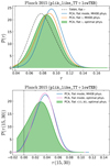 |
Fig. 4. Constraints on the total optical depth (top panel), and on the optical depth between z = 15 and z = 30 (bottom panel), when using 2015 PlanckTT+lowTEB data. Various reionization models and priors are used (labeled in each plot), in addition to marginalization over other ΛCDM parameters. Top panel: apparent preference for higher τ when using the PCA model as reported in Heinrich et al. (2017) was significantly impacted by the choice of prior. Bottom panel: evidence for early reionization was also partly impacted, although some preference remains. We consider the shaded green contour, which corresponds to a flat τ prior and optimal physicality region, as the most well-motivated constraint from this dataset. |
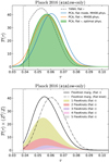 |
Fig. 5. Constraints on the total optical depth when using the Planck intermediate simlow likelihood alone. Various reionization models and priors are used (labeled in each plot), with other ΛCDM parameters fixed to their best-fit values from PlanckTT data. In the bottom panel, the height of each FlexKnot model is proportional to its Bayesian evidence, with an overall scaling so that their sum (the black curve) gives a properly normalized probability distribution. This curve corresponds to marginalization over the number of FlexKnot to use. |
5. Reionization from Planck intermediate data
The Planck polarization likelihood used in the previous section and by Heinrich et al. (2017) and Heinrich & Hu (2018) is the most recent public Planck likelihood available and is based on polarization maps from Planck-LFI data (Planck Collaboration II 2016). Reionization constraints from lower-noise HFI data were presented in an intermediate release (Planck Collaboration Int. XLVI 2016). Additionally, Planck Collaboration Int. XLVII (2016) also explored various parametric reionization models extending beyond just the TANH case. In general, good consistency with a near-instantaneous transition was found, and the optical depth constraints tightened and shifted to lower central values of τ ≈ 0.055–0.060, with σ(τ) ∼ 0.01. Although no evidence for early reionization was found, no completely generic reconstruction was performed, and the parametric models considered did not fully accommodate an early component should one have been present (Heinrich et al. 2017). We thus give here results from a fully generic reconstruction of the reionization history using the simlow likelihood.
So as to most clearly judge the impact of the large-scale polarization data, we compute constaints using only simlow. To do so, we fix non-reionization cosmological parameters to their best-fit values from the high-ℓ TT data, in particular holding the quantity 109Ase−2τ fixed (which better approximates the impact of the TT data as compared to holding just As fixed). The black dashed contour in the top panel of Fig. 5 shows constraints on τ from simlow assuming the TANH model, as also presented in Planck Collaboration Int. XLVI (2016) and Planck Collaboration Int. XLVII (2016). Note that a significant part of the posterior density is cut off by Gunn-Peterson bound requiring full reionization by z = 6, which for the TANH model translates to τ > 0.0430. Due to the finite width of reionization assumed in the TANH case (Δz = 0.5), this is slightly higher than the absolute minimum possible for instantaneous reionization at z = 6, which is τ > 0.0385. The remaining lines show results using the PCA model and various choices of prior. As before, when flattening the τ prior we see a downward shift in τ. Switching to the optimal physicality priors now mostly has the effect of removing some weight at τ < 0.0385, which before was unphysically allowed by the MH08 region. Switching to the optimal physicality region remedies some of this effect and gives (21)
(21)
This is in good agreement with the TANH result, as well as those from the parametric models of Planck Collaboration Int. XLVII (2016).
In the bottom panel of Fig. 5, we show constraints from the FlexKnot model. In all cases except for the dot-dashed line, we use a flat prior on τ. The posteriors on τ with varying numbers of knots are shown as the shaded contours. Each posterior has been normalized to unity then multiplied by 𝒵0/𝒵i, where 𝒵i is the evidence for that number of knots and 1/𝒵0 = ∑i1/𝒵i. This means that the height of each curve is proportional to the evidence of that model, and makes it easy to see that the 1-knot model has most evidence, and the evidence decreases for all subsequent models. Summing up these curves produces the posterior on τ marginalized over the number of knots, which is shown in black, and is properly normalized to unity by the choice of 𝒵0. In this case we find (22)
(22)
This as well is in very good agreement with the results above, demonstrating the lack of evidence in the simlow data for anything other than a single late and near-instantaneous transition to a fully ionized universe.
Even more directly, we show in Fig. 6 the posterior constraints on the history itself using the FlexKnot model, marginalized over the number of knots. Here we see the tight restriction on any amount of non-zero ionization fraction at high redshifts, independent of exactly which τ prior we use. Indeed, the posterior on the z > 15 contribution to the optical depth is bounded to be (23)
(23)
Although we consider the FlexKnot result more robust than the PCA one, we also compute the PCA bound on this quantity to stress that the disappearance of the hints of early reionization in the intermediate Planck data is more related to the data rather than the model used. Even in the PCA case, we find (24)
(24)
which is weaker but still largely rules out the central value of even the prior-adjusted results given by Planck 2015 data (Eq. (20)).
Of course, the FlexKnot model is not immune to choice of τ prior. For comparison, we show as the dot-dashed line in Fig. 5 the FlexKnot result, marginalized over knots, but with a flat prior on the knot positions and amplitudes instead of a flat prior on τ. We find (25)
(25)
which is 0.4σ higher than the result with a flat τ prior (Eq. (22)). We regard this difference as quantifying an unavoidable systematic uncertainty in τ due to imperfect knowledge of the model parameter priors which is inherent in fully generic reconstructions of the reionization history. In the next section, we consider the impact of this uncertainty on other cosmological parameters that are correlated with τ, both from current and future data.
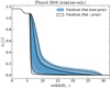 |
Fig. 6. Constraints on the ionization fraction as a function of redshift from simlow-only data, using either a flat prior on the knot positions or a flat prior on τ. The blue and black contours represent the middle 68% and 95% quantile of the posterior at each redshift. |
6. Impact on future data
We now turn to forecasting the impact of reionization uncertainty on future data. There are two question we would like to answer. The first is whether the increased errors bars on τ when performing a generic reconstruction cause any significant degradation in constraints on other parameters of interest. In the case of Fig. 5 we see around a 25% larger error bar in the FlexKnot case as compared to the TANH case7. We will check the impact of this degradation, as well as forecasting whether this can be improved upon with better data. Secondly, we will take the shift in the τ posterior between a flat knot prior and a flat τ prior and propagate it into shifts on other parameters of interest given future data, to check the extent to which these future constraints are prior-dependent. In our discussion, we focus on the sum of neutrino masses, Σmν, as it is the cosmological parameter expected to be most impacted by the details of reionization (Allison et al. 2015).
The first dataset we consider is a combination of CMB-S4 with existing Planck data (including the intermediate simlow likelihood). We perform a Fisher forecast using the standard procedure (Dodelson 2003), using a fiducial Planck 2015-like cosmology, with τ = 0.055 and Σmν at the minimum value of 60 meV. For CMB-S4, we assume a temperature noise level  , a fraction of covered fsky = 0.5, and a beam size of θFWHM = 3arcmin. For the noise levels of the reconstructed lensing deflection power spectrum, we use the noise power spectrum calculated by Pan & Knox (2015)
8 based on an iterative quadratic EB estimator (Okamoto & Hu 2003; Smith et al. 2012). We assume the largest scales measurable by CMB-S4 are ℓmin = 50. This is combined with the constraints on τ from simlow discussed in the previous section, which are treated as independent. In combining with the remaining Planck 2015 data, to take into account correlations between Planck and CMB-S4 due to sky coverage and multipole overlap, we compute a Planck-like Fisher forecast rather than use the real Planck constraints. The temperature and polarization noise levels assumed for Planck are those given by Planck Collaboration (2006), taking an optimal noise weighting of the 100, 143, and 217 GHz, channels, and a sky coverage of fsky = 0.75. These reproduce the uncertainties on parameters from the real Planck data to within around 15%, which should be good enough for our purposes.
, a fraction of covered fsky = 0.5, and a beam size of θFWHM = 3arcmin. For the noise levels of the reconstructed lensing deflection power spectrum, we use the noise power spectrum calculated by Pan & Knox (2015)
8 based on an iterative quadratic EB estimator (Okamoto & Hu 2003; Smith et al. 2012). We assume the largest scales measurable by CMB-S4 are ℓmin = 50. This is combined with the constraints on τ from simlow discussed in the previous section, which are treated as independent. In combining with the remaining Planck 2015 data, to take into account correlations between Planck and CMB-S4 due to sky coverage and multipole overlap, we compute a Planck-like Fisher forecast rather than use the real Planck constraints. The temperature and polarization noise levels assumed for Planck are those given by Planck Collaboration (2006), taking an optimal noise weighting of the 100, 143, and 217 GHz, channels, and a sky coverage of fsky = 0.75. These reproduce the uncertainties on parameters from the real Planck data to within around 15%, which should be good enough for our purposes.
For this first dataset, we forecast a 1σ error bar on Σmν of 59.9 meV assuming the TANH model, or 66.0 meV with the 25% looser τ prior coming from the FlexKnot model. This fairly modest degradation is depicted by the error bars labeled P16+S4 in Fig. 7. What about the impact from the 0.4σ shift in τ depending on the prior assumed? The Fisher methodology allows us to propagate this into a shift in Σmν via (26)
(26)
where ρ is the correlation coefficient between τ and Σmν. For the P16+S4, we find ρ = 0.8, thus the shift in Σmν is 0.3σ. This is depicted by the black arrow in Fig. 7. It is arbitrarily chosen to point to lower Σmν, which is the direction of shift we would expect when going from a flat knot prior to a flat τ prior.
The existence of this shift is a main conclusion from this work, and has not been considered before. To the extent that both flat knot and flat τ priors are reasonable, this can be considered as an extra source of “model uncertainty” in the future CMB determination of neutrino mass. The magnitude of the effect is not disastrous, but not negligible either. We comment now on a few avenues to reduce its impact.
The first comes from adding in other expected future constrains from measurements of the baryon acoustic oscillations (BAO) feature in the galaxy correlation function by DESI (Levi et al. 2013). We use the Fisher matrix for DESI calculated by Pan & Knox (2015), based on the sensitivities presented in Font-Ribera et al. (2014). The addition of this dataset brings us significantly closer to a guaranteed detection of the neutrino mass. Here we find a 1σ error bar on Σmν of 26.3 meV or 28.8 meV, again depending on the reionization model used9. Although the error bars shrink, the addition of DESI actually increases the correlation between τ and Σmν slightly to ρ = 0.9. This arises because DESI is completely insensitive to the τ − As degeneracy responsible for the correlation, but reduces other physical degeneracies impacting the Σmν determination, thus leaving the former degeneracy more prominent. In this case, we find a 0.35σ shift in Σmν depending on the τ prior used. While this is a larger relative shift, on an absolute scale it is about half the shift as compared to without DESI.
To reduce ρ and thus the impact of reionization uncertainty, we need data which directly constrains τ and/or As. This could be provided, for example, by more precise large-scale polarization data. There is room for some improvement as the Planck data is not yet at the cosmic variance limit. We thus consider the limiting case of a full-sky cosmic-variance limited EE measurement across multipoles 2–30 (which we will label cvlowEE). This should be the upper bound of what could be achieved with next-generation satellite missions, e.g. LiteBIRD, PIXIE, COrE, or PICO (Matsumura et al. 2016; Kogut et al. 2011; The COrE Collaboration 2011). To obtain the most accurate forecasts, we run MCMC chains using the exact full-sky Cℓ likelihood (e.g. Hamimeche & Lewis 2008). This is more accurate than Fisher forecasts, which do not easily deal with the sharp edges of the physicality priors. Using the TANH model, we forecast an error bar of (27)
(27)
and with the FlexKnot model marginalized over the number of knots, we obtain (28)
(28)
This leads to a 15% degradation of the error bar in Σmν, somewhat better than the 25% degradation we found previously with simlow. Additionally, ρ is reduced to 0.5, meaning the shift in Σmν due to the choice of τ prior is now only 0.2σ. Evidently, these improved large-scale polarization measurements would be quite valuable, not just for reducing the absolute uncertainty on τ, but also for reducing our dependence on its prior.
When we combine all datasets discussed thus far, including both cvlowEE and DESI-BAO, we find an expected constraint of ~15 meV, with the τ prior able to shift things only by ~3 meV. This would be enough for a ∼4σ guaranteed detection of non-zero neutrino masses even if the true value is at the minimum.
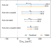 |
Fig. 7. Fisher forecasted 1σ error bars on the sum of neutrino masses, Σmν, assuming a fiducial value at the minimum allowed sum of 60 meV. Different datasets are labeled on the left, with P16 corresponding to Planck 2015 data combined with the intermediate simlow likelihood, S4 corresponding to CMB-S4, BAO to DESI-BAO, and cvlowEE to a cosmic-variance-limited full-sky EE measurement up to ℓ = 30. Orange error bars use the TANH reionization model, and blue errors bars are slightly degraded due to having marginalized over all possible reionization histories via the FlexKnot model. The black arrows show the expected shift when considering a flat knot prior vs. a flat τ prior. |
7. Discussion and conclusions
In this work we have examined the impact of priors on generic reconstruction of the reionization history. We have pointed out some problems with PCA procedure, mainly that (1) the priors that are usually taken over the mode amplitudes correspond implicitly to a somewhat informative prior on τ and (2) a sub-optimal set of physicality priors has been used to-date. Ultimately, the dependence of the final posterior on the details of these physicality priors argues that the PCA procedure is not well suited to this problem. This is not to say there are issues with PCA analyses in general, simply that in situations where hard priors exist and are informative (such as here), the PCA method is a sub-optimal tool. Indeed, we have shown the significant extent to which some of these priors have impacted the analysis of Heinrich et al. (2017) and Heinrich & Hu (2018), artificially increasing the significance of some hints of a high-redshift reionization component.
Even so, the PCA analysis can still be quite useful in providing a simple and convenient approximate likelihood as described in Heinrich et al. (2017). One can then easily project different physical models onto the principal components to obtain constraints on the physical model parameters, effectively applying the priors of the physical model and alleviating some of the problems that arise when attempting to interpret the PCA results on their own.
We have also described the FlexKnot model, which we argue is better to use in a completely generic reionization reconstruction setting since physicality can be enforced exactly and the question of how many knots to use can be self-consistently dealt with via a Bayesian evidence computation.
Using these models, we have presented the first generic reconstruction results from the Planck 2016 intermediate simlow likelihood. We find no evidence for early reionization, instead only very tight upper limits on any contribution at z ≳ 15. This is true even when using the as-argued sub-optimal PCA model, thus the qualitative conclusion of preference only for a late and fast reionization is quite robust to modeling choices. These results negate the need for explanations of an early reionization contribution, for example from metal-free stars (Ahn et al. 2012; Miranda et al. 2017), and can instead be used to place constraints on these scenarios.
Recently, the EDGES collaboration has detected an absorption feature in the sky-averaged spectrum, presumably due to 21 cm absorption by neutral hydrogen during the epoch of reionization (Bowman et al. 2018). In the standard picture, the upper and lower frequencies of the feature indicate that photons from early stars were numerous enough to equilibrate the gas temperature and 21cm spin temperature near z = 20, and then raise the spin temperature above the CMB temperature near z = 15. Due to the amplitude and shape of the detected feature, however, some non-standard explanation is required. The results discussed here can limit such possible explanations, as no modifications to the standard picture must be made which would lead to reionizing the universe to a level large enough to violate the bound on the optical depth at z > 15 given in Eq. (23). For example, Ewall-Wice et al. (2018) discuss an explanation of the EDGES signal in which a radio background from accretion onto the black hole remnants of metal-free stars causes the absorption feature to appear deeper against the continuum than in the standard scenario. It is shown that X-rays also produced by the accretion would result in some significant reionization at z > 15, already in some tension with even the high τ(15, 30) obtained by Heinrich & Hu (2018); given the tighter upper bounds we find here, this explanation is now heavy disfavored in its simplest form.
Regardless of the generic reconstruction models we consider, we find there is some sensitivity to whether a flat prior on τ is taken, or one which is flat on PCA mode amplitudes or knot positions and/or amplitudes. Other priors for this problem exist as well, for example Jeffreys priors or reference priors (Jeffreys 1946; Bernardo 1979), and these would be well worth exploring too. Nevertheless, it is unclear that a very strong argument could be made for which particular prior is the correct one. Thus here we instead take the shifts in τ we find when switching between the priors we have considered as an unavoidable modeling uncertainty arising from the generic reconstruction.
We showed that this uncertainty can have significant impact on determination of the sum of neutrino masses from future experiments. For example, different priors can cause a shift of 0.35σ on Σmν from future Planck + CMB-S4 + DESI-BAO measurements. One avenue for improvement would be to obtain something approaching a cosmic-variance-limited measurement of large-scale CMB polarization. Some other avenues exist as well.
For example, several direct constraints exist on the ionization state of the universe at various redshifts (summarized, e.g. by Bouwens et al. 2015). Here we have applied only one of them, mainly the stringent bound on the end of reionization from observations of the Gunn-Peterson optical depth in high-redshift quasars. We have done so in a fairly unsophisticated way by simply requiring that  . A more detailed study of the impact that these direct constraints have is warranted.
Another approach is to use physically motivated models of reionization, rather than the generic unphysical reconstruction methods presented here. These could potentially shrink the prior parameter space further to where priors become unimportant. The challenge here is finding models which have parameters that can be marginalized over to accurately represent uncertainty as to the physics of reionization and the types of sources which can contribute ionization radiation. In addition, with physical models, we may better be able to fold in constraints from other sources, such as measurements of the patchy kinetic Sunyaev-Zeldovich effect which can further constrain reionization (Gruzinov & Hu 1998; Knox et al. 1998; Zahn et al. 2012; Planck Collaboration Int. XLVII 2016; Park et al. 2013). We have not applied these bounds here as it is not straightforward how to do so for the generic reionization histories we consider, but in principle these could reduce our dependence on priors. Additionally, using novel analysis methods (Smith & Ferraro 2017; Ferraro & Smith 2018), experiments like CMB-S4 could potentially measure this effect to high significance. Further down the road, methods described in Liu et al. (2016) or Meyers et al. (2018) could also push beyond the CMB cosmic variance limit we have calculated and remove the uncertainty on other cosmological parameters due to τ entirely. Future prospects are thus optimistic, although work remains to be done.
There is a small residual ionization level on the order of 10−4 remaining after recombination. We ignore this as the data considered here is insensitive to it.
For clarity, we suppress writing the integration limits zmin and zmax for the rest of the paper. The exact normalization is purely a definitional choice. Similarly, the distinction of special orthonormal basis, i.e. that S is purely a rotation, is not usually made, but we choose to do so here for definiteness and for aiding the subsequent geometrical interpretation.
Pandolfi et al. (2011) use a physicality prior such that the ionization fraction must be physical at all redshifts, which is equivalent to (incorrectly) limiting m1 assuming m2 = 0. This rules out value of m1 which are not inherently unphysical, and thus potentially biases results.
Note that in dimensions higher than the two depicted in Fig. 1, this region does not necessarily have equal edge length in all directions, and is thus truly a hyperbox as opposed to a hypercube.
Equivalently, we could modify the hypersphere prior to be centered on the physicality region rather than on the origin, but we choose to discuss this in terms of picking a different xfid simply for convenience so that Eq. (5) is unchanged.
One small difference is that Heinrich et al. (2017) use the full TT, TE, and EE data, whereas here we use only the “robust” TT data. We have checked that this makes a very small difference to the conclusions in this section, as expected since the TT data is much more constraining.
We compute the TANH error bar here by taking the standard deviation the TANH posterior. Despite that this is clearly non-Gaussian as it is cut off by the Gunn-Peterson prior, it gives us a rough estimate to use in combination with Fisher forecasts.
Provided by the authors upon request.
These predictions are slightly less optimistic than the ones presented in the main body of Pan & Knox (2015), mostly because we use ℓmin = 50 for CMB-S4 as opposed to ℓmin = 2 used there. They are in better agreement with Allison et al. (2015) which take a similar ℓmin, but still very slightly wider, due mostly to a lower fiducial value of τ.
Acknowledgments
We thank Zhen Pan for his forecasting code which we adapted to use in this work, Torsten Ensslin, Douglas Scott, and Martin White for their helpful comments on the draft of this paper, and Silvia Galli, William Handley, and Wayne Hu for useful discussions. MM was supported by the Labex ILP (reference ANR-10-LABX-63). This work was aided by the use of several software packages, including CAMB (Lewis et al. 2000), CosmoSlik (Millea 2017), getdist (Lewis & Xu 2016), Julia (Bezanson et al. 2017), and PolyChord (Handley et al. 2015a,b).
References
- Abazajian, K. N., Arnold, K., Austermann, J., et al. 2015, Astropart. Phys., 63, 66 [NASA ADS] [CrossRef] [Google Scholar]
- Abazajian, K. N., Adshead, P., Ahmed, Z., et al. 2016, ArXiv e-prints, [arXiv:1610.02743] [Google Scholar]
- Ahn, K., Iliev, I. T., Shapiro, P. R., et al. 2012, ApJ, 756, L16 [NASA ADS] [CrossRef] [Google Scholar]
- Allison, R., Caucal, P., Calabrese, E., Dunkley, J., & Louis, T. 2015, Phys. Rev. D, 92, 123535 [NASA ADS] [CrossRef] [Google Scholar]
- Becker, R. H., Fan, X., White, R. L., et al. 2001, AJ, 122, 2850 [NASA ADS] [CrossRef] [Google Scholar]
- Bernardo, J. M. 1979, J. Royal Stat. Soc. Ser. B (Methodological), 41, 113 [Google Scholar]
- Bezanson, J., Edelman, A., Karpinski, S., & Shah, V. 2017, SIAM Rev., 59, 65 [Google Scholar]
- Bouwens, R. J., Illingworth, G. D., Oesch, P. A., et al. 2015, ApJ, 811, 140 [NASA ADS] [CrossRef] [Google Scholar]
- Bowman, J. D., Rogers, A. E. E., Monsalve, R. A., Mozdzen, T. J., & Mahesh, N. 2018, Nature, 555, 67 [NASA ADS] [CrossRef] [Google Scholar]
- Colombo, L. P. L., & Pierpaoli, E. 2009, New Ast., 14, 269 [NASA ADS] [CrossRef] [Google Scholar]
- Dodelson, S. 2003, Moder n Cosmology (Amsterdam: Academic Press) [Google Scholar]
- Ewall-Wice, A., Chang, T. C., & Lazio, J., et al. 2018 ApJ, submitted [arXiv:1803.01815] [Google Scholar]
- Fan, X., Narayanan, V. K., Strauss, M. A., et al. 2002, ApJ, 123, 1247 [NASA ADS] [CrossRef] [Google Scholar]
- Ferraro, S., & Smith, K. M. 2018, ArXiv e-prints, [arXiv:1803.07036] [Google Scholar]
- Font-Ribera, A., McDonald, P., Mostek, N., et al. 2014, JCAP, 2014, 023 [NASA ADS] [CrossRef] [Google Scholar]
- Gruzinov, A., & Hu, W. 1998, ApJ, 508, 435 [NASA ADS] [CrossRef] [Google Scholar]
- Hamimeche, S., & Lewis, A. 2008, Phys. Rev. D, 77, 103013 [NASA ADS] [CrossRef] [Google Scholar]
- Handley, W., & Millea, M. 2018, Bayesian Analysis, submitted [arXiv:1804.08143] [Google Scholar]
- Handley, W. J., Hobson, M. P., & Lasenby, A. N. 2015a, MNRAS, 450, L61 [NASA ADS] [CrossRef] [Google Scholar]
- Handley, W. J., Hobson, M. P., & Lasenby, A. N. 2015b, MNRAS, 453, 4385 [NASA ADS] [CrossRef] [Google Scholar]
- Hazra, D. K., & Smoot, G. F. 2017, JCAP, 11, 028 [NASA ADS] [CrossRef] [Google Scholar]
- Heinrich, C., & Hu, W. 2018, ArXiv e-prints, [arXiv:1802.00791] [Google Scholar]
- Heinrich, C. H., Miranda, V., & Hu, W. 2017, Phys. Rev. D, 95, 023513 [NASA ADS] [CrossRef] [Google Scholar]
- Hu, W., & Holder, G. P. 2003, Phys. Rev. D, 68, 023001 [NASA ADS] [CrossRef] [Google Scholar]
- Jeffreys, H. 1946, Proc. Roy. Soc. London Ser. A, Math. Phys. Sci., 186, 453 [Google Scholar]
- Knox, L., Scoccimarro, R., & Dodelson, S. 1998, Phys. Rev. Lett., 81, 2004 [NASA ADS] [CrossRef] [Google Scholar]
- Kogut, A., Fixsen, D. J., Chuss, D. T., et al. 2011, JCAP, 07, 025 [NASA ADS] [CrossRef] [Google Scholar]
- Levi, M., Bebek, C., Beers, T., et al. 2013, ArXiv e-prints, [arXiv:1308.0847] [Google Scholar]
- Lewis, A., & Xu, Y. 2016, Cmbant/Getdist: 0.2.6, Tech. rep., Zenodo. [Google Scholar]
- Lewis, A., Challinor, A., & Lasenby, A. 2000, ApJ, 538, 473 [Google Scholar]
- Lewis, A., Weller, J., & Battye, R. 2006, MNRAS, 373, 561 [NASA ADS] [CrossRef] [Google Scholar]
- Li, S. 2011, J. Math. Stat., 4, 66 [Google Scholar]
- Liu, A., Pritchard, J. R., Allison, R., et al. 2016, Phys. Rev. D, 93, 043013 [NASA ADS] [CrossRef] [Google Scholar]
- Matsumura, T., Akiba, Y., Arnold, K., et al. 2016, J. Low Temp. Phys., 184, 824 [NASA ADS] [CrossRef] [Google Scholar]
- Meyers, J., Meerburg, P. D., van Engelen, A., & Battaglia, N. 2018, Phys. Rev. D, 97, 103505 [NASA ADS] [CrossRef] [Google Scholar]
- Millea, M. 2017, Astrophysics Source Code Library [record ascl:1701.004] [Google Scholar]
- Miranda, V., Lidz, A., Heinrich, C. H., & Hu, W. 2017, MNRAS, 467, 4050 [NASA ADS] [CrossRef] [Google Scholar]
- Mortonson, M. J., & Hu, W. 2008a, ApJ, 672, 737 [NASA ADS] [CrossRef] [Google Scholar]
- Mortonson, M. J., & Hu, W. 2008b, ApJ, 686, L53 [NASA ADS] [CrossRef] [Google Scholar]
- Obied, G., Dvorkin, C., Heinrich, C., Hu, W., & Miranda, V. 2018, Phys. Rev. D, 98, 043518 [NASA ADS] [CrossRef] [Google Scholar]
- Okamoto, T., & Hu, W. 2003, Phys. Rev. D, 67, 083002 [NASA ADS] [CrossRef] [Google Scholar]
- Pan, Z., & Knox, L. 2015, MNRAS, 454, 3200 [NASA ADS] [CrossRef] [Google Scholar]
- Pandolfi, S., Ferrara, A., Choudhury, T. R., Melchiorri, A., & Mitra, S. 2011, Phys. Rev. D, 84, 123522 [NASA ADS] [CrossRef] [Google Scholar]
- Park, H., Shapiro, P. R., Komatsu, E., et al. 2013, ApJ, 769, 93 [Google Scholar]
- Planck Collaboration 2006, ArXiv e-prints [arXiv:astro-ph/0604069] [Google Scholar]
- Planck Collaboration II. 2016, A&A, 594, A2 [NASA ADS] [CrossRef] [EDP Sciences] [Google Scholar]
- Planck Collaboration XX. 2016, A&A, 594, A20 [NASA ADS] [CrossRef] [EDP Sciences] [Google Scholar]
- Planck Collaboration Int. XLVI. 2016, A&A, 596, A107 [NASA ADS] [CrossRef] [EDP Sciences] [Google Scholar]
- Planck Collaboration Int. XLVII. 2016, A&A, 596, A108 [NASA ADS] [CrossRef] [EDP Sciences] [Google Scholar]
- Planck Collaboration Int. LI.2017, A&A, 607, A95 [NASA ADS] [CrossRef] [EDP Sciences] [Google Scholar]
- Smith, K. M., & Ferraro, S. 2017, Phys. Rev. Lett., 119, 021301 [NASA ADS] [CrossRef] [Google Scholar]
- Smith, K. M., Hanson, D., LoVerde, M., Hirata, C. M., & Zahn, O. 2012, JCAP, 2012, 014 [Google Scholar]
- The COrE Collaboration (Armitage-Caplan, C., et al.) 2011, ArXiv e-prints, [arXiv:1102.2181] [Google Scholar]
- Vázquez, J. A., Bridges, M., Hobson, M. P., & Lasenby, A. N. 2012, JCAP, 06, 006 [NASA ADS] [CrossRef] [Google Scholar]
- Villanueva-Domingo, P., Gariazzo, S., Gnedin, N. Y., & Mena, O. 2018, JCAP, 04, 024 [NASA ADS] [CrossRef] [Google Scholar]
- Zahn, O., Reichardt, C. L., Shaw, L., et al. 2012, ApJ, 756, 65 [Google Scholar]
Appendix A: Maximum entropy prior flattening
Here we will show how to construct the maximum entropy prior used in Sect. 3.2. This is the maximally uninformative prior on the input parameters of our model, (θ1, θ2, …), for which the induced prior on τ = τ(θ1, θ2, …) is flat. Here, the θi can represent the PCA model amplitudes, the knot positions and/or amplitudes, or any other parameters.
We first begin with a simplified example: what is the maximum entropy prior on two parameters, a and b, each with support on 0 < a, b < 1, for which the prior on the sum, a + b, is flat between 0 < a + b < 2? In this analogy, a and b are the θi parameters, a + b is like τ, and the support on [0,1] is the physicality region.
The entropy of the probability distribution p(a, b) is![Mathematical equation: $ \begin{aligned} H[p(a,b)] \,{=}\, - \int _0^1 \text{ d}a \int _0^1 \text{ d}b \, p(a,b) \ln p(a,b). \end{aligned} $](/articles/aa/full_html/2018/09/aa33288-18/aa33288-18-eq51.gif) (A.1)
(A.1)
We can express the problem of finding the p(a, b) which maximizes H, subject to some constraints, as a Lagrange multiplier problem. Our constraint is that the transformed probability distribution for the sum, p(a + b), is flat. We will write this constraint in what may seem as an odd form, but which is conducive to solving the Lagrange multiplier problem. We will require that the moments of p(a, b) with respect to a + b are those of a flat distribution between 0 and 2. This is to say, that ⟨a + b⟩ = 1, ⟨(a + b)2⟩ = 8/3, etc...By specifying an infinite number of moments, we guarantee our target distribution p(a + b) is exactly flat. Our constraints are thus that (A.2)
(A.2)
with (A.3)
(A.3)
for all n = 0…∞. Note that for n = 0 we simply have that the integral over p(a, b) is unity, which guarantees that it is a probability distribution. Higher moments fix p(a + b) to be flat as desired. As a Lagrange multiplier problem, we are maximizing the functional,![Mathematical equation: $ \begin{aligned} F[p(a,b)] \,{=}\,&\int _0^1 \text{ d}a \int _0^1 \text{ d}b \;\Biggl \{ -p(a,b) \ln p(a,b) \nonumber \\&+ \sum _{i\,{=}\,0}^\infty \lambda _i \left[(a+b)^n p(a,b) - c_n \right]\Biggr \}, \end{aligned} $](/articles/aa/full_html/2018/09/aa33288-18/aa33288-18-eq54.gif) (A.4)
(A.4)
where the λi are the Lagrange multipliers. Setting the variation of F with respect to p(a, b) to zero gives us that![Mathematical equation: $ \begin{aligned} p(a,b) \,{=}\, \exp \left[-1+\sum _{i\,{=}\,0}^\infty \lambda _i (a+b)^n\right]. \end{aligned} $](/articles/aa/full_html/2018/09/aa33288-18/aa33288-18-eq55.gif) (A.5)
(A.5)
Substituting this into each of the Eq. (A.2) could then be used to solve for all of the λi, giving us the unique maximum entropy solution for p(a, b). Rather than preforming this process explicitly, we will postulate the answer and show that it is the solution. Consider the probability distribution (A.6)
(A.6)
where q(a + b) is the transformed probability distribution for a + b given the initial flat priors on a and b, (A.7)
(A.7)
It is straightforward to substitute this into Eq. (A.6) and then show that p(a + b) is indeed flat between 0 and 2. This means it satisfies the infinite number of constraint equations. It remains to check that the variation of F around this function is zero, which is tantamount to showing that it can be written in the form of Eq. (A.5). Since Eq. (A.5) says that the log of our function is a Maclaurin series in a + b and since our p(a, b) is an elementary function of only a + b, this is also true. Therefore, we have shown Eq. (A.5) is the unique maximum entropy probability distribution of a, b for which the transformed distribution of a + b is flat.
The above proof trivially generalizes to N variables and to any initial support by simply adding in more integrals and changing the limits to something other than 0 and 1. Similarly, one can easily replace a + b with any desired function for a derived parameter. This proof thus applies to the case of flattening the τ prior discussed in Sect. 3.2. For a more rigorous and general proof, see Handley & Millea (2018).
All Figures
|
Fig. 1. Geometric picture of the PCA physicality priors in two-dimensions, demonstrating why they necessarily allow unphysical regions of parameter space. The solid blue square is the physicality region in terms of the ionization fraction, x1 and x2, at individual redshifts. The solid orange square is the physicality region in terms of the mode amplitudes, m1 and m2. The two types of physicality priors corresponding to Eq. (4) and Eq. (5) are shown as the dashed square and dashed circle, respectively. Their intersection, shaded orange, is the full physicality region. The left panel takes a fiducial ionization history, xfid = 0.15, consistent with Mortonson & Hu (2008a) and subsequent works. The right panel shows that the undesired but allowed unphysical parameter space can be reduced (but not fully) with a better choice of fiducial model. |
| In the text | |
|
Fig. 2. One thousand reionization histories sampled from their prior distribution given the different models we consider. In the PCA case, the prior over PCA modes is taken to be uniform within the physicality region; in the two knot cases, the prior is uniform on the position and/or amplitude of each knot (thus none of these priors correspond to a flat τ priors). The left panel shows the extent to which the PCA procedure allows unphysical models, even when using the optimal physicality priors. The middle panel shows that the HS17 prior creates odd features and tighter peaked priors in the regions between the knot locations (which are indicated with arrows). The right panel is the prior for the FlexKnot model and represents our best solution for creating a reasonable and “homogeneous” prior. |
| In the text | |
|
Fig. 3. Solid colored lines: implicit prior on τ from the PCA model when taking a flat prior on the mode amplitudes, computed via Monte Carlo. The top panel assumes the MH08 physicality region, whereas the bottom panel assumes our optimal physicality region. In the case of the bottom panel, analytic calculation of the prior is possible via Eq. (15) and shown as dotted lines. The top panel also shows the implicit prior for the HS17 model. |
| In the text | |
|
Fig. 4. Constraints on the total optical depth (top panel), and on the optical depth between z = 15 and z = 30 (bottom panel), when using 2015 PlanckTT+lowTEB data. Various reionization models and priors are used (labeled in each plot), in addition to marginalization over other ΛCDM parameters. Top panel: apparent preference for higher τ when using the PCA model as reported in Heinrich et al. (2017) was significantly impacted by the choice of prior. Bottom panel: evidence for early reionization was also partly impacted, although some preference remains. We consider the shaded green contour, which corresponds to a flat τ prior and optimal physicality region, as the most well-motivated constraint from this dataset. |
| In the text | |
|
Fig. 5. Constraints on the total optical depth when using the Planck intermediate simlow likelihood alone. Various reionization models and priors are used (labeled in each plot), with other ΛCDM parameters fixed to their best-fit values from PlanckTT data. In the bottom panel, the height of each FlexKnot model is proportional to its Bayesian evidence, with an overall scaling so that their sum (the black curve) gives a properly normalized probability distribution. This curve corresponds to marginalization over the number of FlexKnot to use. |
| In the text | |
|
Fig. 6. Constraints on the ionization fraction as a function of redshift from simlow-only data, using either a flat prior on the knot positions or a flat prior on τ. The blue and black contours represent the middle 68% and 95% quantile of the posterior at each redshift. |
| In the text | |
|
Fig. 7. Fisher forecasted 1σ error bars on the sum of neutrino masses, Σmν, assuming a fiducial value at the minimum allowed sum of 60 meV. Different datasets are labeled on the left, with P16 corresponding to Planck 2015 data combined with the intermediate simlow likelihood, S4 corresponding to CMB-S4, BAO to DESI-BAO, and cvlowEE to a cosmic-variance-limited full-sky EE measurement up to ℓ = 30. Orange error bars use the TANH reionization model, and blue errors bars are slightly degraded due to having marginalized over all possible reionization histories via the FlexKnot model. The black arrows show the expected shift when considering a flat knot prior vs. a flat τ prior. |
| In the text | |
Current usage metrics show cumulative count of Article Views (full-text article views including HTML views, PDF and ePub downloads, according to the available data) and Abstracts Views on Vision4Press platform.
Data correspond to usage on the plateform after 2015. The current usage metrics is available 48-96 hours after online publication and is updated daily on week days.
Initial download of the metrics may take a while.