| Issue |
A&A
Volume 617, September 2018
|
|
|---|---|---|
| Article Number | A131 | |
| Number of page(s) | 13 | |
| Section | Extragalactic astronomy | |
| DOI | https://doi.org/10.1051/0004-6361/201833261 | |
| Published online | 02 October 2018 | |
“Zombie” or active? An alternative explanation to the properties of star-forming galaxies at high redshift
1
INAF – Osservatorio Astronomico di Roma, Via Frascati 33, 00040 Monte Porzio Catone, RM, Italy
e-mail: This email address is being protected from spambots. You need JavaScript enabled to view it.
2
Space Science Data Center, Agenzia Spaziale Italiana, Via del Politecnico snc, 00133 Roma, Italy
3
ASTRON – Netherlands Institute for Radio Astronomy, Oude Hoogeveensedijk 4, 7991 Dwingeloo, The Netherlands
4
Dipartimento di Fisica, Università degli Studi di Roma ‘La Sapienza’, P.le A. Moro 5, 00185 Roma, Italy
5
INFN, Sezione di Roma I, P.le A. Moro 2, 00185 Roma, Italy
6
Dipartimento di Fisica, Università di Roma “Tor Vergata”, Via della Ricerca Scientifica 1, 00133 Roma, Italy
7
Department of Astronomy, University of Maryland, College Park, MD 20742, USA
8
NASA/Goddard Space Flight Center Code 662, Greenbelt, MD 20771, USA
Received:
19
April
2018
Accepted:
18
June
2018
Abstract
Context. Star-forming galaxies at high redshift show anomalous values of infrared excess, which can be described only by extremizing the existing relations between the shape of their ultraviolet continuum emission and their infrared-to-ultraviolet luminosity ratio, or by constructing ad hoc models of star formation and dust distribution.
Aims. We present an alternative explanation, based on unveiled AGN activity, of the existence of such galaxies. The scenario of a weak AGN lends itself naturally to explain the observed spectral properties of these high-z objects in terms of a continuum slope distribution and not altered infrared excesses.
Methods. To this end, we directly compare the infrared-to-ultraviolet properties of high-redshift galaxies to those of known categories of AGN (quasars and Seyferts). We also infer the characteristics of their possible X-ray emission.
Results. We find a strong similarity between the spectral shapes and luminosity ratios of AGN with the corresponding properties of such galaxies. In addition, we derive expected X-ray fluxes that are compatible with the energetics from AGN activity.
Conclusions. We conclude that a moderate AGN contribution to the UV emission of such high-z objects is a valid alternative to explain their spectral properties. Even the presence of an active nucleus in each source would not violate the expected quasar statistics. Furthermore, we suggest that the observed similarities between anomalous star-forming galaxies and quasars may provide a benchmark for future theoretical and observational studies on the galaxy population in the early Universe.
Key words: galaxies: ISM / galaxies: photometry / infrared: galaxies / ultraviolet: galaxies / galaxies: active / quasars: general
© ESO 2018
1. Introduction
The estimate of the galactic dust content and properties in objects at high redshift (z > 5) is crucial for assessing the details of the star formation history in galaxies. However, it is not always feasible to obtain the measurement of the far-infrared (FIR) flux emission, due to low instrumental sensitivity or lack of spectral coverage (e.g., Bouwens et al. 2014, 2016; Rogers et al. 2014; Finkelstein et al. 2015a,b; Bowler et al. 2015; Capak et al. 2015; Barišić et al. 2017, Under the assumption of radiative equilibrium, it is possible to correlate the FIR emission to the amount of ultraviolet (UV) flux absorbed by dust and reprocessed at longer wavelengths since the dust extinction of reasonable absorption models peaks in the UV band (Weingartner & Draine 2001; Bianchi & Schneider 2007; Draine 2011). Therefore, it is common practice to quantify the extinction at such redshifts using the galaxy-emission properties in the rest-frame UV band (Bouwens et al. 2014, 2015; Finkelstein et al. 2015a).
The recent detection of FIR emission from high-z galaxies (z > 5; Finkelstein et al. 2015a,b; Bowler et al. 2015; Capak et al. 2015; Waters et al. 2016; Bouwens et al. 2016; Knudsen et al. 2017) provides better constraints on their dust properties, such as extinction. In particular, the study of galaxies with non-negligible star formation rates (SFRs) shows that their intrinsic wavelength spectral index βint, i.e., the slope of the power-law spectrum used to describe the galactic UV emission, is nearly constant with values between −2.5 and −2.3 (Meurer et al. 1999; Wilkins et al. 2013; Bouwens et al. 2014; Reddy et al. 2015; Forrest et al. 2016; Mancini et al. 2016; Narayanan et al. 2018; Reddy et al. 2018; Popping et al. 2017; Cullen et al. 2017), although Reddy et al. (2015), Casey et al. (2014) and Forrest et al. (2016) found a value compatible with β > −2.3 and Talia et al. (2015) estimated β ∼ −3.02.
Meurer et al. (1999) initially suggested the possibility of correlating the difference between the observed and the expected β, which is used to describe the galactic UV continuum, to the extinction coefficient at 1600 Å (hereafter A1600). This procedure is made possible by the independence of the intrinsic spectrum of star-forming galaxies from the stellar-population age and by its weak correlation with the stellar metallicity (see, e.g., Meurer et al. 1999; Mancini et al. 2015, and references therein). Furthermore, it is possible to correlate A1600 with the infrared excess (IRX) defined as
 (1)
(1)
where LFIR is the FIR galactic luminosity integrated from 8 μm to 1000 μm and LUV is the monochromatic luminosity at 1600 Å in the rest frame. The IRX-to-β relation obtained in this way only depends on the dust mass (i.e., the normalization of the dust-extinction law), the dust properties (i.e., the shape of such a law), and the intrinsic spectral index βint corrected for the dust absorption.
This relation appears to be universal for star-forming galaxies (e.g., Meurer et al. 1999). However, Capak et al. (2015) observed a population of high-z star-forming galaxies that appear to strongly deviate from the usual relations, showing lower IRX with respect to that expected on the basis of their observed spectral slope. These sources were selected to measure [C II] gas and dust emission in Lyman-break galaxies (LBGs) detected in the 2 deg2 Cosmological Evolution Survey (COSMOS; Scoville et al. 2007) in order to explore the average properties of the interstellar medium (ISM) at high redshift. The reanalysis of the Capak et al. (2015) data done by Barišić et al. (2017) partially relaxed the tension between their IRXs and spectral slopes, but without eliminating it, especially for the case of upper limits to the IRX. These objects populate a region of the IRX–β plane that is typical of quiescent galaxies with negligible or no star formation (“dead”) despite having SFRs from tens to hundreds of M⊙ yr−1 as measured by their [C II] emission (Capak et al. 2015), and could therefore be denoted as “zombie” galaxies.
Several scenarios have been proposed to explain how star-forming galaxies can deviate from the usual IRX-to-β relations (Bouwens et al. 2016; Ferrara et al. 2017; see also Ouchi et al. 1999). However, the observed discrepancy with the predicted IRXs would either imply a strong bias in the determination of the dust temperature (Bouwens et al. 2016) or extreme physical conditions in the dust clouds (Ferrara et al. 2017). In this work, we formulate the alternative hypothesis that the high-z galaxies with anomalous IRX-to-β discovered by Capak et al. (2015) are actually hosting AGN activity. This scenario allows us to consider objects in which the UV flux is dominated by accretion-disk processes (e.g., Salpeter 1964; Zel’dovich & Novikov 1965; Shakura & Sunyaev 1973) and in which the intrinsic UV spectral slope depends on the properties of the central engine (accretion rate, black hole mass, black hole spin) and is therefore not limited to steep values (e.g., Shankar et al. 2016). In this way, the Capak et al. (2015) objects are no longer constrained to have anomalous dust properties, but are instead located in the region of the IRX–β plane corresponding to their AGN UV continuum.
The paper is organized as follows. In Sect. 2 we exploit the idea developed by Capak et al. (2015) that AGN activity is responsible for the altered IRX-to-β of the high-z galaxies. We present a tentative statistical classification of these objects based on their spectral properties in Sect. 3. We also compute the expected X-ray emission from AGN with properties similar to these sources in Sect. 4, and compare the fluxes estimated in this way with the current X-ray upper limits of these sources derived from Chandra observations of the COSMOS field. Finally, we summarize and discuss our findings in Sect. 5. Throughout the text, we use “AGN” to indicate both low- and high-luminosity objects, and adopt a concordance cosmology with H0 = 70 km s−1 Mpc−1, ΩM = 0.3, and ΩΛ = 0.7.
2. The IRX-to-β relation for AGN
The sample of 16 high-z galaxies discovered by Capak et al. (2015) is presented in Table 1. It comprises six single sources (HZ1, HZ2, HZ3, HZ4, HZ7, and HZ9), and four multiple systems (HZ5, HZ6, HZ8, and HZ10) that are probably composed of interacting objects. Their redshifts were measured through absorption-line spectroscopy with the instrument DEIMOS at the Keck Observatory. For all but one of them (HZ5a), the measurements or at the least upper limits of their UV spectral slope and IRX are given in Barišić et al. (2017). In the following, we adopt this data set for our analysis of such objects in search of AGN behavior.
Basic properties of the high-z galaxies discovered by Capak et al. (2015) and reanalyzed by Barišić et al. (2017).
In order to validate the hypothesis that star-forming galaxies at high redshift with anomalous IRX-to-β values are hosts of AGN activity, we first define a comparison sample of AGN that has measurements of UV to optical spectral slopes β, IR luminosities LIR, and UV luminosities LUV. We find that Dong & Wu (2016) constructed such a catalog for quasars, i.e., AGN with Lbol ≳ 1045 erg s−1. A similar catalog has been constructed by García-González et al. (2016) for nearby (DL < 70 Mpc) Seyfert galaxies (Lbol ≲ 1045 erg s−1). By comparing both catalogs to the Capak et al. (2015) galaxies, we are able to span five orders of magnitude in bolometric luminosity from 1043 to 1048 erg s−1, thus covering a wide range of AGN energetics.
We note that the selection criteria used in these AGN catalogs significantly differ from those adopted by Capak et al. (2015) and Barišić et al. (2017), due to the diverse purposes for which the samples were constructed (the study of the link between AGN activity and host-galaxy star formation in the case of Dong & Wu 2016, and the disentanglement of the FIR emission due to AGN activity from that due to star formation in García-González et al. 2016). Nevertheless, a comparison between AGN and the Capak et al. (2015) objects based on the average properties of such samples is still feasible because we focus on spectral properties that are nearly unhindered by the nature of the ISM gas. For instance, the zombie galaxy HZ5, though satisfying the object selection performed by Capak et al. (2015), is actually a weak Type 1 quasar (Brightman et al. 2014; Kalfountzou et al. 2014). Therefore, we expect that the different selection criteria among the three samples do not greatly affect our findings.
2.1. Construction of a quasar comparison sample
The quasar catalog by Dong & Wu (2016) is composed of objects from the Sloan Digital Sky Survey Data Release 7 (SDSS-DR7; Abazajian et al. 2009; Schneider et al. 2010; Shen et al. 2011) and Data Release 10 (SDSS-DR10; Ahn et al. 2014; Pâris et al. 2014) that were observed in the FIR domain by the Spectral and Photometric Imaging Receiver (SPIRE) on board the Herschel Space Observatory in the framework of the Herschel Stripe 82 Survey (HerS; Viero et al. 2014). This survey covers ∼29% (79 deg2) of the SDSS Stripe 82 (270 deg2 on the celestial equator in the southern Galactic cap; Adelman-McCarthy et al. 2007) with FIR observations at 250, 350, and 500 μm.
The joint HerS/SDSS sample includes 207 quasars with the following characteristics:
UV to optical ugriz magnitudes from the SDSS;
near-IR (NIR) JHKs magnitudes from the 2MASS Skrutskie et al. and UKIDSS (Lawrence et al. 2007) surveys;
mid-IR (MIR) fluxes from the AllWISE catalog (Wright et al. 2010; Mainzer et al. 2011) ranging from 3.4 to 22 μm;
Herschel FIR flux measurements in the passbands centered at the wavelengths mentioned above.
The spectral energy distribution (SED) of each object has been decomposed in several spectral components, each accounting for the emission from a different source: a power law for the quasar accretion disk, two near- to mid-IR bumps peaking at around 2–4 μm and 10–20 μm for the radiation reprocessed by the dusty torus, two galaxy templates (Sb for the young stellar component and E for the old one) for the host-galaxy contribution, a Small Magellanic Cloud (SMC) reddening law and a “graybody” radiation with power-law emissivity for the FIR excess. In this way, Dong & Wu (2016) measured IR and UV luminosities for each quasar in the sample, along with the corresponding frequency spectral slope α which is related to the wavelength slope β by
 (2)
(2)
Thanks to the SED analysis, the HerS/SDSS catalog also provides information on several other quasar and host-galaxy parameters, such as the virial black hole (BH) mass MBH derived from single-epoch relations (Vestergaard & Peterson 2006; Vestergaard & Osmer 2009; Shen & Kelly 2010) and the mass of cold gas Mgas stored in the AGN surrounding environment. The former is measured by adopting the quasar continuum luminosities computed from the power-law emission, while the latter is estimated from the long-wavelength tail of the dust emission (see Scoville et al. 2014, for details).
Since the SED decomposition in multiple components allows us to measure quasar intrinsic reddening, this may be used to correct the quantities derived from the fitting procedure. Therefore, LUV and β given in the HerS/SDSS sample are intrinsic to the quasars, whereas the corresponding observed quantities (i.e., with no correction for internal reddening applied) are needed in the construction of the IRX-to-β relation. In order to recover the observed LUV and β, we apply backward the de-reddening procedure adopted by Dong & Wu (2016). We individually de-correct both LUV and β through a SMC extinction template (Pei 1992) scaled to the value of intrinsic reddening Aint of each quasar, and use these reddened quantities in the evaluation of the quasar IRX-to-β relation.
The resulting sample of quasar IRX and spectral slopes is shown in Fig. 1. At first glance, it is evident as all but three high-z galaxies by Capak et al. (2015) fall inside the region of the IRX–β diagram populated by quasars. For comparison, we compute the IRX-to-β relations by Pettini et al. (1998) and Meurer et al. (1999) for several values of the intrinsic spectral slope βint from −2.5 to −1, and show them superimposed on the observed IRX-to-β values for high-z galaxies and quasars.
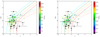 |
Fig. 1. IRX–β plane for quasars. The data corresponding to the high-z galaxies by Capak et al. (2015) reanalyzed by Barišić et al. (2017) are shown (black squares), along with their 1σ errors, superimposed on the HerS/SDSS quasars (filled dots). The empirical IRX-to-β relations by Pettini et al. (1998, dashed lines) and Meurer et al. (1999, solid lines) computed for values of βint from −2.5 to −1 are also reported. Left panel: HerS/SDSS quasars segregated in logarithmic MBH. Right panel: HerS/SDSS quasars segregated in logarithmic Mgas. Only HerS/SDSS objects with measured MBH and Mgas are used. |
It should be noted that the HerS/SDSS quasars tend to segregate in the IRX–β plane according to both their MBH (left panel of Fig. 1) and Mgas (right panel of Fig. 1). In particular, quasars hosting more massive black holes have lower IRXs, whereas objects with higher gas masses show steeper intrinsic slopes coupled to slightly higher IRXs. It is unclear whether the tendency for quasars with higher MBH to have lower IRXs is due to a physical mechanism such as quasar feedback (e.g., Cattaneo et al. 2009; Fabian 2012), since the main driver of feedback appears to be the quasar Eddington ratio Lbol/Ledd rather than the black hole mass (Ricci et al. 2017b; see also Ishibashi & Fabian 2016; Ishibashi et al. 2017). Such a segregation could equally be produced by a selection bias in the observation of quasars with massive black holes, for example by preferentially finding objects with bluer spectra at the high end of the MBH distribution due to their lower Eddington ratio.
Conversely, a high Mgas may be associated with gas-rich quasar surrounding environments, resulting in high-luminosity objects which tend to have bluer spectra and hence steeper βint (e.g., Shankar et al. 2016). Since high gas masses also enhance the star formation and dust content of the host galaxy (e.g., Kennicutt & Evans 2012), the tendency of quasars with higher Mgas to segregate towards steeper UV spectral slopes and higher IRXs is explained by the simultaneous presence of a higher AGN and stellar luminosity, and a higher dust mass. We note that future observations of high-z galaxies could benefit from using these tendencies as diagnostics to infer the presence of a centrally located AGN powering part of the UV emission.
2.2. Construction of a Seyfert comparison sample
The Seyfert comparison sample has been constructed in García-González et al. (2016) by selecting objects from the Revised Shapley–Ames (RSA) catalog (Sandage & Tammann 1987) that were identified as Seyfert galaxies by Maiolino & Rieke (1995). These objects were selected in order to have Herschel/Photometric Array Camera (PACS) imaging in at least two bands and SPIRE photometric observations. The final catalog by García-González et al. (2016) comprises 33 galaxies (15 Sy 1 and 18 Sy 2), of which we only use those with near- and far-UV (NUV and FUV) magnitudes available in the literature in order to compute UV spectral slopes and luminosities. We therefore select Seyfert galaxies from this catalog by performing a search on the NASA Extragalactic Database1 (NED) for objects with both NUV and FUV measurements.
Our final sample is composed of 19 Seyferts with
NUV and FUV AB magnitudes measured by the Galaxy Evolution Explorer (GALEX) satellite for UV surveys (Martin et al. 2005; Gil de Paz et al. 2007);
MIR spectroscopy with high angular resolution (see García-González et al. 2016, and refs. therein);
Herschel FIR photometric measurements from 70 μm to 500 μm.
All these objects have IR SEDs fitted by García-González et al. (2016) with graybody components which allow us to compute LFIR. Coupling these luminosities to the UV magnitudes, we are able to compute the IRX for this subsample, which we show in Fig. 2 as a function of the corresponding β compared to the high-z galaxies by Capak et al. (2015). A visual inspection reveals that these Seyferts have shallower UV spectral slopes and higher IRXs with respect to quasars, thus populating the region at −1 ≲ β ≲ 0 and IRX ≳ 0 which contains neither high-z galaxies nor HerS/SDSS quasars (see Fig. 1). This suggests that a possible AGN activity in the Capak et al. (2015) objects must have properties closer to efficient high-luminosity AGN than to weak ones.
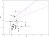 |
Fig. 2. IRX–β plane for Seyfert galaxies. The data by Barišić et al. (2017) are shown (black squares), along with their 1σ errors, superimposed on the sample of Seyfert galaxies by García-González et al. (2016 magenta crosses). For comparison, the theoretical IRX-to-β relation by Meurer et al. (1999) with βint = −2.23 (solid line) and the relation by Pettini et al. (1998) with βint = −2 (dashed line) are also reported. |
2.3. Estimate of the galactic UV contribution
The scenario in which the high-z galaxies by Capak et al. (2015) host AGN activity with average spectral properties (i.e., βint ∼ −2 once a correction for the dust reddening is taken into account in evaluating the spectral slope; Dong & Wu 2016) holds well in describing the observed IRX-to-β distribution of such objects. However, a residual galaxy contribution to the total UV flux cannot be neglected, since models of AGN and host-galaxy coupling, derived from numerical simulations (e.g., Schneider et al. 2015), show that the AGN emission accounts on average for 30% to 70% of the system’s UV energetics. Therefore, we tried to reproduce the observed values of IRX and β for the high-z galaxies with a hybrid relation that takes into account both the AGN and host-galaxy UV contribution.
Equation (1) can be rewritten in a form that only depends on the fraction D(τλ,β) of reprocessed UV light L1600 into IR radiation and on the UV dust reddening S(τλ,β). In doing this, we obtain LUV = L1600 · S(τλ,β), LFIR = L1600 · D(τλ,β) and
![Mathematical equation: $${\rm IRX}\,{=}\,\log{\left[ \frac{L_{\rm 1600}\,{\cdot}\,D(\tau_\lambda,\beta)}{L_{\rm 1600}\,{\cdot}\,S(\tau_\lambda,\beta)} \right]}\,{=}\,\log{\left[\frac{D(\tau_\lambda,\beta)}{S(\tau_\lambda,\beta)} \right]}\cdot $$](/articles/aa/full_html/2018/09/aa33261-18/aa33261-18-eq19.gif) (3)
(3)
The reprocessed UV fraction D(τλ,β) and the reddening S(τλ,β) are respectively given by
 (4)
(4)
and
 (5)
(5)
where β is the intrinsic slope of the UV spectrum and τλ is the wavelength-dependent optical depth of the dust distribution.
Since the AGN (through accretion-disk emission) and the host galaxy (through star formation) both heat the dust that reprocesses the UV into FIR emission, we can separate the contributions to the IRX by writing
![Mathematical equation: $${\rm IRX}\,{=}\,\log{\left\{ \frac{ L^{\rm (q)}_{\rm 1600}\,{\cdot}\,D\left[\tau^{\rm (q)}_\lambda,\beta_{\rm q}\right] + L^{\rm (g)}_{\rm 1600}\,{\cdot}\,D\left[\tau^{\rm (g)}_\lambda,\beta_{\rm g}\right] }{ L^{\rm (q)}_{\rm 1600}\,{\cdot}\,S\left[\tau^{\rm (q)}_\lambda,\beta_{\rm q}\right] + L^{\rm (g)}_{\rm 1600}\,{\cdot}\,S\left[\tau^{\rm (g)}_\lambda,\beta_{\rm g}\right] } \right\}}, $$](/articles/aa/full_html/2018/09/aa33261-18/aa33261-18-eq22.gif) (6)
(6)
where βq and βg are the AGN and host-galaxy UV spectral slopes respectively. Defining fq as the fraction of energy injected in the dust by the AGN, we get
![Mathematical equation: $$f_{\rm q}\,{=}\,\frac{ L^{\rm (q)}_{\rm 1600}\,{\cdot}\,S\left[\tau^{\rm (q)}_\lambda,\beta_{\rm q}\right]}{ L^{\rm (q)}_{\rm 1600}\,{\cdot}\,S\left[\tau^{\rm (q)}_\lambda,\beta_{\rm q}\right] + L^{\rm (g)}_{\rm 1600}\,{\cdot}\,S\left[\tau^{\rm (g)}_\lambda,\beta_{\rm g}\right] }$$](/articles/aa/full_html/2018/09/aa33261-18/aa33261-18-eq23.gif) (7)
(7)
and finally, combining Eqs. (3), (6), and (7),
![Mathematical equation: $$ {\rm IRX}\,{=}\,\log{\left[ f_{\rm q}\,{\cdot}\,10^{{\rm IRX}_{\rm q}}+ \left( 1-f_{\rm q} \right)\,{\cdot}\,10^{{\rm IRX}_{\rm g}}\right]}.$$](/articles/aa/full_html/2018/09/aa33261-18/aa33261-18-eq24.gif) (8)
(8)
We adopt the functional form by Pettini et al. (1998) with βint = −2 in order to describe the IRXq. This model is in fact valid if the dust distribution is foreground to the UV source (e.g., Gordon et al. 1997; Inoue 2005; Gallerani et al. 2010), which is suggested for AGN by unified scenarios where a clumpy distribution of obscuring dust surrounds the central engine (e.g., Urry & Padovani 1995; Risaliti et al. 2011; Krumpe et al. 2014). For IRXg, we adopt the Meurer et al. (1999) IRX-to-β relation with βint = −2.23, since in galaxies the dust is expected to be mixed with stars rather than being (almost) completely foreground (Calzetti 1997; Pettini et al. 1998; Meurer et al. 1999). In order to cover the whole average range of AGN contributions to the total UV emission, we choose for fq the extreme values of 0.3 and 0.7 (Schneider et al. 2015).
Figure 3 shows such combined IRX-to-β relations, along with the pure relations by Pettini et al. (1998) and Meurer et al. (1999). The relations with 30%–70% UV contribution from AGN emission do not fully describe any of the data by Barišić et al. (2017), while the Meurer et al. (1999) relation partially intercepts the observations at IRX ≳ 0 and the Pettini et al. (1998) relation partially succeeds in describing the bulk of observations at −1 < IRX < 0 and −2 < β < −1. Overall, an IRX-to-β relation with both an AGN and galactic contribution to the UV emission appears to be the most suitable to simultaneously describe the spectral properties of Seyferts, quasars, and star-forming galaxies at high redshift. The posterior distribution of least-squares fits of Eq. (8) performed over bootstrap realizations of the total data set by Barišić et al. (2017, high-z galaxies with anomalous IRX), Dong & Wu (2016, HerS/SDSS quasars), and García-González et al. (2016, local Seyferts) with fq as the only free parameter gives fq = 0.73 ± 0.11, compared with a value of fq = 0.70 ± 0.12 obtained by fitting only the AGN-dominated objects.
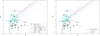 |
Fig. 3. Left panel: theoretical IRX-to-β relations for mixed AGN and host-galaxy UV contributions. A |


2.4. Intrinsic reddening estimates of the high-z galaxies
Under the assumption that the Capak et al. (2015) galaxies are actual observations of AGN hosts that exactly follow an IRX-to-β relation with AGN contribution, it is now possible to derive the unattenuated AGN spectral slopes  using the measured IRX and the observed UV slopes βobs. In order to obtain these values, we evaluate Eq. (8) for each high-z galaxy with fq between 0.3 and 1, fixing the intrinsic slope for the galactic contribution
  at −2.23 (Meurer et al. 1999) and adopting as our fiducial estimate the value of
  for which the composite IRX-to-β relation intercepts each data point. In particular, we find that the lowest AGN contribution (i.e., fq = 0.3) is the most reasonable choice to reproduce the observed IRX-to-β values for the four leftmost objects in the IRX-to-β diagram, namely HZ4, HZ9, HZ10, and HZ10W. This choice of fq predicts values of
  between −5.7 and −2.8 for such objects; higher values of the AGN contribution would predict even steeper intrinsic AGN UV slopes or would fail to reproduce the observed data.
The remaining objects are instead well reproduced if we set a complete AGN domination in the UV flux (i.e., fq = 1). Lower values of fq lead the composite IRX-to-β relation to intercept the region between the IRX-to-β fiducial values below  . An AGN-dominated UV spectrum allows us instead to reproduce the data of HZ1, HZ2, HZ3, HZ6b, and HZ6c with a single relation at
  ; we recall that this is the average value of the intrinsic UV slopes for AGN (Dong & Wu 2016). Furthermore, such a relation also describes the remaining objects assuming
  .
.
We then use the βint derived in this way along with the HST/WFC3 data by Barišić et al. (2017) in order to obtain an estimate of the UV extinction A1600 affecting the AGN emission. To do this, we adopt the simplified assumption that the bolometric luminosities of these objects are approximated using the optical/UV bolometric corrections by Runnoe et al. (2012b). Therefore, we estimate the optical monochromatic luminosities at 3000 Å from the F160W magnitudes by Barišić et al. (2017), and apply the corrections listed in Table 1 of Runnoe et al. (2012a) to derive the de-reddened UV luminosities at 1600 Å. The choice of indirectly computing such luminosities through the correction of the optical magnitudes is motivated by the fact that, at least for low to moderate values of A1600, the luminosity at optical wavelengths is less affected by extinction than the UV flux.
Under these hypotheses, we define the values of A1600 by assuming that the intrinsic UV slopes of the objects by Capak et al. (2015) are reddened by an SMC-like extinction. Such extinction coefficients are shown in Fig. 4 as a function of  , suggesting that the possible AGN emission of these high-z galaxies is affected on average by low to moderate reddening along the line of sight (A1600 ≲ 1.2 mag).
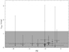 |
Fig. 4. Extinction coefficient A1600 as a function of the intrinsic spectral slope |

2.5. Possible issues in the comparison between different samples of extragalactic sources
Although the presented analysis focuses on the comparison among the average emission properties of the sample of high-z star-forming galaxies by Capak et al. (2015) with those of two AGN classes, the dependence of the latter on quantities derived from SED fitting can bias the results due to (i) the availability of different models for the paramount spectral components , (ii) the possible parameter degeneracies arising in the SED construction, and (iii) the adoption of peculiar extinction curves. In the following, we briefly describe the expected impact of these biases on the main findings reported in this section.
Model dependencies. Model dependencies are particularly important in fitting the main sources of UV (e.g., the details of the AGN process and its ionized surrounding environment) and IR emission (e.g., the reprocessing of radiation by dust in the AGN’s surrounding environment). For instance, the AGN emission may be reproduced by either using a UV template to take into account the additional light from resolved emission lines and Fe II blending (García-González et al. 2016) or adopting a simple power-law functional form (Dong & Wu 2016). However, the difference in such approaches generates discrepancies of ≲10% only in the determination of the UV flux from AGN, i.e., the average contribution of emission features to the total emission with respect to the continuum (e.g., Vanden Berk et al. 2001; Glikman et al. 2006), and hence is not expected to have a great impact on the derivation of the source’s properties unless tailoring the selection for objects with extreme line emission. On broader wavelength ranges, the differences introduced by SEDs related to different emission models can directly affect the determination of IRX, UV slope, and dust extinction. Duras et al. (2017) show that there are some differences among quasar SEDs, but these are in general compatible with each other within at most 0.5 dex on a wavelength range of 100–106 Å (see, e.g., their Figs. 2 and 3), apart from some peculiar choices (e.g., Stalevski et al. 2016). Additionally, the largest discrepancies in the IR emission are due to the opening angle of a dusty AGN torus (Stalevski et al. 2016; Duras et al. 2017), but they are again limited to ∼0.5 dex. A shift of ∼±1 dex in the IRX of AGN introduced by SED differences is still compatible with the observed IRXs of the zombie galaxies by Capak et al. (2015), thus not greatly biasing our main results.
Degeneracies. Another problem is the degeneracies among the free parameters involved in the SED-fitting procedure, which can be explored in detail only with the availability of rich data sets in order to give statistical significance to the fit results (see, e.g., Mullaney et al. 2011). For instance, the UV SED of a quasar affected by intrinsic reddening could be reproduced by either assuming a shallow UV slope (thus neglecting the dust extinction) or an appropriate extinction law applied to a steep spectrum (β ∼ −2; e.g., Dong & Wu 2016). In the FIR, both the dust emission from the host galaxy and the emission from a possible old stellar population peak at ∼100 μm, thus making it difficult to disentangle quasar and galaxy light. Dong & Wu (2016) overcome these issues by adopting quasar-galaxy mixing diagrams (Hao et al. 2013) that allow us to distinguish AGN-dominated sources from galaxy-dominated and reddened SEDs. Additionally, they also fix some SED parameters to typical literature values, such as the AGN torus temperature at 1300 K and the slope of the graybody emissivity for galactic dust at 1.6 in order to reduce possible secondary degeneracies. On the other hand, García-González et al. (2016) rely on spectro-photometric indicators such as the fν(70 μm)/fν(160 μm) flux ratio and the equivalent width of polycyclic aromatic hydrocarbon (PAH) features to discriminate between galaxy emission and AGN activity. Therefore, we can assume that parameter degeneracies are already taken into account in the adopted AGN samples, thus not affecting their comparison with the properties of the zombie galaxies.
Dust extinction. Regarding the choice of the extinction curve, we have already outlined that taking into account different extinction curves and dust distribution geometries do not help reconcile the expected behavior of the zombie galaxies in the IRX–β plane, as widely described in the literature (see, e.g., Mancini et al. 2016; Narayanan et al. 2018; Ferrara et al. 2017; Behrens et al. 2018, and references therein). In particular, the work by Narayanan et al. (2018) suggests that in order to have a galaxy that covers the same locus of the zombie galaxies these object would need a spectral emission dominated by an old stellar population. Alternatively, Ferrara et al. (2017) suggest that it is possible to reduce the discrepancy between the observed and expected IRXs by considering a stellar population completely embedded in a molecular cloud phase. However, even in this strong condition, it is not possible to completely explain the FIR upper limits measured by Capak et al. (2015) and Barišić et al. (2017). Another possibility is to consider a highly inhomogeneous dust distribution produced by dust accretion of surface metals (e.g., Mancini et al. 2016), which would produce higher values of β at the same IRXs. Nevertheless, this effect is not strong enough to reconcile the theoretical expectations of UV slopes and FIR emission with the observed behavior of the zombie galaxies, particularly the upper limits in the IRX at β ≳ −1.5 (see Mancini et al. 2016, for further details). Therefore, we remark that the existence of a weak AGN activity at the center of such high-z objects appears to be a more reasonable explanation for their peculiar IRX-to-β values.
3. Color-magnitude relation for AGN
The difficulty to reproduce the IRX-to-β relation for the sources by Capak et al. (2015) within the scenario of galaxy-dominated objects can be avoided by assuming that these sources are actually hosting AGN activity with UV spectral emission depending on the details of the accretion process. Figures 1–3 show how a UV spectrum with βint not fixed to galactic values may explain the bulk of the data after the reanalysis by Barišić et al. (2017). If this alternative scenario holds, these objects should also follow typical relations that are known for AGN, such as showing steeper spectral slopes at higher luminosities (e.g., Shankar et al. 2016).
Figure 5 shows β as a function of MUV for the HerS/SDSS quasars, the Seyfert galaxies by García-González et al. (2016), and the high-z galaxies by Capak et al. (2015). In order to quantify the β-to-MUV relation for AGN, we perform a Monte Carlo linear regression by running the script PyMC3 (Salvatier et al. 2016) on the joint sample of quasar and Seyfert spectral slopes β as a function of their UV absolute magnitude MUV. We choose a standard likelihood defined as
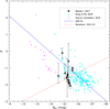 |
Fig. 5. Color-magnitude relation for the HerS/SDSS quasars by Dong & Wu (2016, cyan dots), the Seyfert galaxies by García-González et al. (2016, magenta crosses), and the high-z galaxies by Barišić et al. (2017, black squares). The β-to-MUV relation derived by fitting the HerS/SDSS quasars (blue solid line) is shown superimposed to the data. For comparison, the relation valid for galaxies at z ∼ 5 (Bouwens et al. 2014, red dashed line) is also shown. |
![Mathematical equation: $$ \mathcal{L}\,{\propto}\,\exp{\left( -\frac{\chi^2}{2} \right)}\,{=}\,\exp{\left\{ - \frac{\left[ \beta -(a\,{\cdot}\,M_{\rm UV}+b) \right]^2}{2 \sigma^2} \right\} } $$](/articles/aa/full_html/2018/09/aa33261-18/aa33261-18-eq34.gif) (9)
(9)
with very broad priors for the parameters a, b, and σ:
 (10)
(10)
where  is the Gaussian distribution of UV magnitudes with a given average μ and variance k2, and
  is its positive side. In this way, we find
 (11)
(11)
where we adopt the average uncertainty in the measurement of β for HerS/SDSS objects as an estimate of the systematic error on the intercept of the color-magnitude relation.
Conversely, the dependence of β on UV emission in star-forming galaxies is mainly determined by the amount of extinction. Therefore, the expected trend is to find shallower spectral slopes in bigger, more luminous, more chemically enriched objects with respect to fainter ones (e.g., Meurer et al. 1999; Bouwens et al. 2014; Finkelstein et al. 2015a,b). Here we adopt the relation inferred by Bouwens et al. (2014) at z ∼ 5 to describe the relation between β and MUV in galaxy-dominated objects,
 (12)
(12)
which exhibits an opposite trend with respect to the relation for AGN.
The sample of objects by Capak et al. (2015) is numerically small if compared to the HerS/SDSS ensemble (207 objects) or the Bouwens et al. (2014) catalog (>4000 objects). Furthermore, a visual inspection of Fig. 5 reveals that this sample tends to cluster around the β-to-MUV relation for high-z galaxies. Nevertheless, we aim to test statistically the probability that these objects are AGN- or galaxy-dominated in terms of relative proximity to one relation with respect to the other. In order to do this, we define a χ2 variable as
 (13)
(13)
where β and σβ refer to the observed slopes with their average errors by Barišić et al. (2017), while βx are the values of UV spectral slopes expected for the Capak et al. (2015) objects using either Eq. (11) (βx = βAGN) or Eq. (12) (βx = βgal) with associated standard deviations σx. The Bayesian probability PAGN for a data point by Barišić et al. (2017) to come from an AGN-dominated object is then
 (14)
(14)
with  for an object having
  with respect to Eq. (11) and
  with respect to Eq. (12). The complementary probability Pgal = 1 − PAGN is thus the probability that the data point represents a galaxy-dominated object. We note that we assume a flat prior on both relations (i.e., the objects by Capak et al. 2015 are not forced to follow a priori one between Eqs. (11) or (12).
We report the probabilities in Table 2 for each of the high-z objects by Barišić et al. (2017). Only HZ5 and HZ8W can be classified as AGN hosts at a 90% confidence level, with HZ5 already recognized as an X-ray selected quasar (Capak et al. 2015), whereas HZ1 to HZ3 and HZ10 are likely to be normal galaxies. The other targets show intermediate values of PAGN, and hence it is not possible to strictly classify them in one category, though all of the objects are enclosed within the scatter of the joint AGN color-magnitude relation. Therefore, no firm conclusion may be drawn about the relative spectral domination of AGN or galaxy emission in the sample of objects by Capak et al. (2015). In order to better distinguish AGN-dominated objects from galaxies, we define as Δβ the distance of the observed β from the β-to-MUV relation for AGN described by Eq. (11),
 (15)
(15)
where βi and  are the UV spectral slope and absolute magnitude for the ith object.
Values of χ2 obtained by comparing the Barišić et al. (2017) data with Eqs. (11) and (12), respectively, along with the corresponding Bayesian probabilities of AGN domination (see text for details).
We show this quantity in Fig. 6 as a function of the IRX for the Dong & Wu (2016), the García-González et al. (2016) and the Barišić et al. (2017) data. It can be seen at first glance that the AGN are clustered by construction around a value of Δβ ∼ 0, and scattered over a range of IRX ∈ [−2,3] with the bulk of the data comprised between IRX ∼ −1 and 2. The objects from Capak et al. (2015) are superimposed on the region covered by actual AGN, with the tendency to populate the lower part of the diagram. Interestingly, segregating these objects by their classification based on Bayesian probability shows that the galaxy-dominated objects (i.e., those objects with Pgal > 0.90) cluster around Δβ ∼ −0.8, while the AGN hosts exhibit positive values of Δβ up to ∼1. This diagram synthesizes all the available information about the emission properties of the Capak et al. (2015) galaxies as reanalyzed by Barišić et al. (2017) since it correlates MUV with the IRX and βobs. We note that this kind of analysis could be used for a preliminary discrimination between AGN hosts and normal star-forming galaxies where a measurement of the FIR emission is feasible, although a more thorough analysis of their UV and FIR properties is needed. Furthermore, the IRX–Δβ plane might also be useful for analyzing the evolution of the local galaxies.
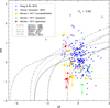 |
Fig. 6. IRX as a function of the slope difference Δβ for the HerS/SDSS quasars by Dong & Wu (2016, blue dots), the Seyfert galaxies by García-González et al. (2016, blue crosses), and the high-z galaxies by Barišić et al. (2017). The high-z galaxies are classified according to the statistical analysis presented in Sect. 3 (red triangles: actual galaxies, yellow squares: unclassifiable objects, green stars: actual quasars). The curves available in the literature that describe the IRX-to-Δβ relation for various classes of galaxies (Pettini et al. 1998; Meurer et al. 1999; Penner et al. 2012; Casey et al. 2014; Talia et al. 2015; Forrest et al. 2016) are also shown. |
To directly compare the effect of removing the AGN dependence on MUV from samples of different objects (quasars, Seyferts, local starbursts, medium-z star-forming galaxies), we rewrite the IRX-to-β relations available in the literature as a function of Δβ = βgal − βAGN. Substituting Eq. (12) into Eq. (11) to eliminate the dependence on MUV and then inverting the result to write βgal as a function of Δβ, we find
 (16)
(16)
Therefore, the IRX-to-Δβ relations assume the form
![Mathematical equation: $$ {\rm IRX}\left( \Delta\beta \right)\,{=}\,\log{\left[ 10^{0.4 \left(m\,{\cdot}\,\Delta\beta + q \right)}-1 \right]}+0.076, $$](/articles/aa/full_html/2018/09/aa33261-18/aa33261-18-eq50.gif) (17)
(17)
with the coefficients m and q depending on the analyzed sample of objects. Unlike in the previous sections of this paper, here we do not restrict ourselves to the relations by Pettini et al. (1998) and Meurer et al. (1999). Instead, we focus on several relations available in the literature that are valid for samples of different classes of galaxies. In Table 3, we list the values of the coefficients m and q for the IRX-to-Δβ relations, along with the source paper of the original IRX-to-β relation and a synthetic description of the corresponding type of astrophysical objects.
Coefficients of the IRX-to-Δβ relations specialized from literature results on different samples of galaxies.
Figure 6 shows these IRX-to-Δβ relations superimposed on the AGN samples and on the high-z galaxies by Capak et al. (2015). Apart from the curve corresponding to the IRX-to-β relation derived by Casey et al. (2014) for star-forming galaxies at z < 0.085, it is evident that none of the considered relations is able to intercept the Capak et al. (2015) galaxies with IRX < 0. This further strengthens the AGN-host hypothesis for the high-z galaxies with anomalous IRXs, and again suggests that deepening the investigation of the IRX–Δβ plane should be a future tool for object discrimination.
4. Expected X-ray luminosities
We now present the analysis of the X-ray emission expected for these objects within the AGN-host scenario. In fact, it has been clearly established that the accretion process around massive black holes can power the emission of X-rays from structures (jets, coronae) collateral to the ionized disk (e.g., Halpern 1982; Begelman et al. 1983; Begelman & McKee 1983; Zdziarski 1985). Therefore, it is possible to select and characterize AGN by studying the details of their high-energy spectra (e.g., Giustini et al. 2008; Lusso et al. 2010; Lusso & Risaliti 2016; Page et al. 2017). In order to give a complete view of the X-ray energetics of the Capak et al. (2015) galaxies, we both evaluate the expected X-ray fluxes of such objects from their measured UV-to-IR properties and perform a stacking analysis on the Chandra X-ray imaging of the COSMOS field at the relevant sky coordinates.
4.1. Estimated upper limits on the X-ray fluxes
The field of the Capak et al. (2015) galaxies has been observed by the Chandra X-ray observatory in the framework of the Chandra COSMOS Survey2 (C-COSMOS; Elvis et al. 2009; Puccetti et al. 2009; Civano et al. 2012; Lanzuisi et al. 2013). This survey has imaged for 1.8 Ms the central region of the COSMOS field around 10h + 02° with an average flux limit of 7.3 × 10⁻¹⁶ erg s−1 cm−2 in the full band (0.5−10 keV). Of the objects listed in Table 1, HZ10 and HZ10W fall outside the area of 0.9 deg2 covered by the C-COSMOS program, and the weak quasar HZ5 is detected as a resolved source. None of the other galaxies in the Capak et al. (2015) sample have been detected.
Assuming that the emission of the non-detected sources in the X-ray comes from AGN-dominated objects, we follow Runnoe et al. (2012b) in computing the bolometric luminosities Lbol of such sources from the values of LUV reported in Table 1. Therefore, we adopt Lbol = fαUVLUV, where the UV-to-bolometric correction is αUV = 5.2, and f = 0.75 is a factor taking into account the anisotropic emission from an accretion disk. The luminosities in the hard (2−10 keV) rest-frame X-ray band LX can then be inferred from the relation obtained by Marconi et al. (2004),
 (18)
(18)
where  . These X-ray luminosity evaluations must be interpreted as upper limits on the intrinsic energetic output of these objects since they would overestimate the real values in the case of non-negligible contribution of the host-galaxy emission in the UV-to-optical band.
Nevertheless, a significant fraction of the observed X-ray emission, especially at low X-ray luminosities (LX ∼ 1043 erg s−1), may be powered by the cumulative radiation produced by high-mass X-ray binaries (HMXBs) in the host galaxy (Ranalli et al. 2003,2005;Lehmer et al.2010,2016). Therefore, we estimate this contribution  in the hard X-ray band following Volonteri et al. (2017), and adopting the redshift-dependent relation found by Lehmer et al. (2016) for galaxies in the redshift range z ∈ [0,7]
 (19)
(19)
where the selected values for z and SFR are shown in Tables 4 and 4, respectively.
We report the predicted luminosities LX and  for the analyzed sample in Table 4. It is clearly visible that, on average, the foreseen luminosities assuming an AGN-driven X-ray emission are ∼2 orders of magnitude higher than the values obtained under the hypothesis of X-ray flux produced by an HMXB population. Even accounting for a host-galaxy contribution of ∼70%, the two predicted emissions still remain very different.
Luminosity properties of the objects described by Capak et al. (2015).
We further note that, at high redshifts, X-ray fluxes can be absorbed by highly obscured environments, such as large amounts of gas and dust surrounding accreting BHs (Ueda et al. 2003; Gilli et al. 2007; Treister et al. 2009). The two main attenuation processes in the X-rays are the photoelectric absorption, accounted for by the cross section σph, and the Compton scattering of photons against free electrons, σT. The photoelectric cross section decreases with increasing energy, and the contribution of the dust to σph is relatively modest for E ≳ 1 keV (Morrison & McCammon 1983). Therefore, at higher energies (E ≳ 10 keV for gas metallicities Z ∼ Z⊙), the energy-independent σT becomes dominant. Softer X-ray photons are thus expected to be more absorbed than harder ones. Furthermore, X-ray observations of AGN at z ≳ 4 typically sample the rest-frame hard X-ray emission, i.e., in the 3–12 keV range on average for the sample by Capak et al. (2015). Even assuming a strong obscuration produced by gas column densities NH ∼ 1023 cm2, the unabsorbed AGN SED for E ≳ 3 keV and Z ≲ 0.1 Z⊙ is at most 1.2 times higher than the absorbed one (see, e.g., Fig. 3 in Pezzulli et al. 2017). The theoretical simulations (Mancini et al. 2016) and observations (Mannucci et al. 2010; Ma et al. 2016) both suggest that the expected metallicity for this kind of objects is ≲0.1 Z⊙. This suggests that neither absorption nor a dominant contribution of the stellar emission to the observed optical photometry is able to reduce the predicted AGN-driven X-ray emission enough to make LX and  comparable. Deeper X-ray observations may greatly help to discriminate between zombie and active galaxies.
4.2. Stacking analysis of the Chandra X-ray imaging
We perform the stacking analysis of the C-COSMOS data at the positions of the remaining sources in order to reveal possible statistical signals, or at least get a flux upper limit that may be useful in order to plan future deep observations with X-ray facilities. For this purpose, we use the software CSTACK, a web-based tool for the stacking analysis of Chandra data developed by T. Miyaji3 (see Appendix A for further details). We only stack sources with an upper limit in LFIR, i.e., HZ1, HZ2, HZ3, HZ5a, HZ7, HZ8, and HZ8W, because the objects with FIR detection could host heavily obscured AGN in which the X-ray emission is almost totally suppressed by the presence of high column densities of gas and IR-emitting dust (e.g., Ricci et al. 2017a). In addition, such objects are the most distant from the traditional IRX-to-β relations adopted for galaxies, further suggesting that their spectral properties can only be explained by AGN domination.
We show the CSTACK output in Fig. 7. While no stacked signal is detected in the hard band, the soft band exhibits an average count rate of (1.95 ± 1.86) × 10−5 cts s−1 in the source region which is not compatible with zero at the 1σ level. However, due to the poor statistics of such a measurement, we are forced to treat it as an upper limit to the X-ray flux rather than a detection. We recall that at z ∼ 5.4, the observer-frame soft band at 0.5 − 2 keV actually observes hard 3−13 keV rest-frame X-rays (for comparison, the observer-frame hard band at 2–8 keV would detect photons produced in the rest-frame range 13–51 keV). Adopting a mean redshift of 5.4, an AGN-typical X-ray photon index Γ ∼ 1.8 (e.g., Trakhtenbrot et al. 2017) and an average Galactic NH ∼ 1.9 × 1020 cm−2 (Dickey & Lockman 1990; Kalberla et al. 2005; McClure-Griffiths et al. 2009; Willingale et al. 2013; HI4PI Collaboration 2016) in the direction of the COSMOS field, the soft-band count rate upper limit of ∼3.8 × 10⁻⁵ cts s−1 derived from the stacking analysis corresponds to an observed flux ≲5.7 × 10⁻¹⁶ erg s−1 cm−2 in the full Chandra band. Interpreting the soft-band excess as a detection, it corresponds to a hard X-ray luminosity of ∼4.6 × 10¹⁰ L⊙ at z ∼ 5.4, in excellent agreement with the luminosities reported in Table 4 for the case of AGN-dominated sources.
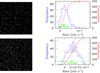 |
Fig. 7. Results of the stacking analysis performed on the C-COSMOS field at the coordinates of the Capak et al. (2015) high-z galaxies given by Barišić et al. (2017, see Table 1). Upper panels: 100″ × 100″ stacked map of the 0.5−2 keV Chandra passband (left) and corresponding count-rate histogram (right). Lower panels: the same for the 2–8 keV Chandra passband. In both histograms, the count-rate frequencies (blue histogram) are shown along their cumulative distributions (red histogram) and their nominal mean (green dot) with 1σ uncertainty. |
5. Discussion
In this paper, we have presented and validated the hypothesis of star-forming galaxies with anomalous IRXs at high redshift (the zombie galaxies) hosting unveiled AGN activity. This alternative scenario to the dust temperature bias (Bouwens et al. 2016) and molecule-rich dust clouds (Ferrara et al. 2017) provides a natural explanation to the IRX-to-β values of such objects in terms of variable intrinsic spectral shape and dust distribution with respect to inactive galaxies.
The comparison of the IR and UV spectral properties of the high-z galaxies discovered by Capak et al. (2015) and reanalyzed by Barišić et al. (2017) with those of quasars (Dong & Wu 2016) and Seyferts (García-González et al. 2016) shows that high-z star-forming galaxies and AGN with bolometric luminosities from 1043 to 1048 erg s−1 populate the same region of the IRX-to-β diagram. Furthermore, we find that the bulk of the data by Barišić et al. (2017) is described by an IRX-to-β relation suitable for AGN-dominated objects with intrinsic spectral slopes around βint ∼ −2 and low galactic contribution to the UV emission (i.e., fq ∼ 0.7), and that this AGN UV flux is moderately reddened (A1600 ≲ 1.2 mag). Model dependencies and degeneracies are already taken into account in the SED fitting of the AGN comparison samples, and are therefore not expected to greatly bias these conclusions (see Sect. 2.5).
We further investigated the possibility of ultimately classifying the anomalous star-forming galaxies from Capak et al. (2015) as actual AGN hosts based on the correlation between their spectral properties, and on their possible X-ray emission. Though superimposing within the scatter to the AGN color-magnitude correlation derived by the Dong & Wu (2016) data, the analyzed objects also lie at the boundary of the calibration region of the color-magnitude relation for inactive galaxies by Bouwens et al. (2014). Therefore, a clear distinction between galaxy-dominated objects and AGN hosts is hard to obtain on the basis of their statistical proximity to one relation with respect to the other. We are in fact only able to classify four objects (HZ1 to HZ3 and HZ10) as normal galaxies and two (HZ5 and HZ8W) as AGN.
Finally, since an analysis of the X-ray emission is crucial in order to definitely assess the nature of such sources, we attempted to derive their expected X-ray luminosities in the opposite cases of AGN domination and galaxy domination, and to detect an X-ray signal from the FIR-undetected objects through stacking analysis. Interestingly, a signal not compatible with zero at the 1σ level arises from stacking the positions of the Capak et al. (2015) objects in the Chandra soft band at 0.5–2 keV, hinting at a possible rest-frame hard X-ray emission from at least some of the sources. According to the luminosities derived in Table 4, such an emission is compatible with the flux expected from AGN-dominated sources at z ∼ 5.4. Hence, future X-ray follow-ups of these objects or surveys through Athena are key to disentangling the two populations of objects.
Our work is based on the hypothesis that all of the zombie galaxies host an AGN at their center. Is this a overly optimistic scenario that would ultimately lead to overestimating the actual number of AGN at z > 5? To test this scenario, we computed the expected AGN amount in the redshift interval probed by the analyzed objects. We adopted the quasar luminosity function by Assef et al. (2011) for the interval 5 < z < 5.85 (see, e.g., their Fig. 7). At those redshifts, the value of the quasar space density is between ∼3.4 × 10⁻⁶ and ∼1.1 × 10⁻⁸ Mpc−3 mag−1 at the 1σ level for sources with −25 < MJ < −22.7 (i.e., the J-band absolute magnitude of the zombie galaxies under the hypothesis of AGN domination), which corresponds to a number of up to 55 high-z quasars in the COSMOS field of view. Restricting the area to the C-COSMOS value of 0.9 deg2 implies a decrease of this amount to ∼25 objects. It should be noted that a NED search for actual quasars at z ∼ 5.4 in the COSMOS field resulted in two sources (SDSS J095728.55+022037.8 and SDSS J100100.04+021300.6; Richards et al. 2009). Therefore, the sample of (at most) 16 high-z objects discovered by Capak et al. (2015) fits inside the currently expected statistics of quasars. This topic will be further exploitable taking advantage of the upcoming releases of COSMOS spectroscopic redshifts (Salvato et al., in prep.)4.
In addition, performing high-precision measurements with the Very Large Baseline Interferometer (VLBI) is an option to probe the radio emission of those objects, aiming at detecting possible jets associated with the accreting AGN (see, e.g., Herrera Ruiz et al. 2017, and references therein). In conclusion, a multiwavelength analysis of such high-redshift objects is not only desirable, but required in order to correctly estimate the star formation history and the evolution of galaxies. To this end, the James Webb Space Telescope (JWST; Gardner et al. 2006; Kalirai 2018), the Wide Field Infrared Survey Telescope (WFIRST; Content et al. 2013), the Atacama Large Millimeter/submillimeter Array (ALMA), and many other facilities play a key role in acquiring new data at z > 5, thus opening new windows to better understand the vast, complex panorama of (mostly unknown) astronomical sources in the high-redshift Universe.
Available at ned.ipac.caltech.edu
An extension of the C-COSMOS program, the 4.6 Ms Chandra COSMOS Legacy Survey (e.g., Marchesi et al. 2016), is present in the literature, but its imaging data are not publicly available for stacking analysis.
Available at http://cstack.ucsd.edu/cstack/ or http://lambic.astrosen.unam.mx/cstack/
We refer to http://cosmos.astro.caltech.edu/page/specz for updates.
Acknowledgments
We are grateful to our anonymous referee for the helpful comments. We thank M. Ginolfi and R. Schneider (University of Rome La Sapienza) for useful discussions. FT acknowledges support from the Programma per Giovani Ricercatori – Anno 2014 “Rita Levi Montalcini”. This research has made use of the NASA/IPAC Extragalactic Database (NED) which is operated by the Jet Propulsion Laboratory, California Institute of Technology, under contract with the National Aeronautics and Space Administration. The development of CSTACK has been supported by CONACyT Grants No. 83564/179662, UNAM-DGAPA Grant PAPIIT IN110209/IN104113/IN104216 and Chandra Guest Observer Support Grant GO1-12178X. The Chandra X-Ray Center (CXC) is operated for NASA by the Smithsonian Astrophysical Observatory.
References
- Abazajian, K. N., Adelman-McCarthy, J. K., Agüeros, M. A., et al. 2009, ApJS, 182, 543 [NASA ADS] [CrossRef] [Google Scholar]
- Adelman-McCarthy, J. K., Agüeros, M. A., Allam, S. S., et al. 2007, ApJS, 172, 634 [NASA ADS] [CrossRef] [Google Scholar]
- Ahn, C. P., Alexandroff, R., Allende Prieto, C., et al. 2014, ApJS, 211, 17 [NASA ADS] [CrossRef] [Google Scholar]
- Assef, R. J., Kochanek, C. S., Ashby, M. L. N., et al. 2011, ApJ, 728, 56 [NASA ADS] [CrossRef] [Google Scholar]
- Barišić, I., Faisst, A. L., Capak, P. L., et al. 2017, ApJ, 845, 41 [NASA ADS] [CrossRef] [Google Scholar]
- Begelman, M. C., & McKee, C. F. 1983, ApJ, 271, 89 [NASA ADS] [CrossRef] [Google Scholar]
- Begelman, M. C., McKee, C. F., & Shields, G. A. 1983, ApJ, 271, 70 [CrossRef] [Google Scholar]
- Behrens, C., Pallottini, A., Ferrara, A., Gallerani, S., & Vallini, L. 2018, MNRAS, 477, 552 [NASA ADS] [CrossRef] [Google Scholar]
- Bianchi, S., & Schneider, R. 2007, MNRAS, 378, 973 [NASA ADS] [CrossRef] [Google Scholar]
- Bouwens, R. J., Illingworth, G. D., Oesch, P. A., et al. 2014, ApJ, 793, 115 [Google Scholar]
- Bouwens, R. J., Illingworth, G. D., Oesch, P. A., et al. 2015, ApJ, 803, 34 [NASA ADS] [CrossRef] [Google Scholar]
- Bouwens, R. J., Aravena, M., Decarli, R., et al. 2016, ApJ, 833, 72 [NASA ADS] [CrossRef] [Google Scholar]
- Bowler, R. A. A., Dunlop, J. S., McLure, R. J., et al. 2015, MNRAS, 452, 1817 [NASA ADS] [CrossRef] [Google Scholar]
- Brightman, M., Nandra, K., Salvato, M., et al. 2014, MNRAS, 443, 1999 [NASA ADS] [CrossRef] [Google Scholar]
- Calzetti, D. 1997, AJ, 113, 162 [NASA ADS] [CrossRef] [Google Scholar]
- Capak, P. L., Carilli, C., Jones, G., et al. 2015, Nature, 522, 455 [NASA ADS] [CrossRef] [Google Scholar]
- Casey, C. M., Scoville, N. Z., Sanders, D. B., et al. 2014, ApJ, 796, 95 [NASA ADS] [CrossRef] [Google Scholar]
- Cattaneo, A., Faber, S. M., Binney, J., et al. 2009, Nature, 460, 213 [NASA ADS] [CrossRef] [PubMed] [Google Scholar]
- Civano, F., Elvis, M., Brusa, M., et al. 2012, ApJS, 201, 30 [NASA ADS] [CrossRef] [Google Scholar]
- Content, D., Aaron, K., Abplanalp, L., et al. 2013, in UV/Optical/IR Space Telescopes and Instruments: Innovative Technologies and Concepts VI, Proc. SPIE, 8860, 88600E [CrossRef] [Google Scholar]
- Cullen, F., McLure, R. J., Khochfar, S., Dunlop, J. S., & Dalla Vecchia, C. 2017, MNRAS, 470, 3006 [NASA ADS] [CrossRef] [Google Scholar]
- Dickey, J. M., & Lockman, F. J. 1990, ARA&A, 28, 215 [NASA ADS] [CrossRef] [MathSciNet] [Google Scholar]
- Dong, X. Y., & Wu, X.-B. 2016, ApJ, 824, 70 [NASA ADS] [CrossRef] [Google Scholar]
- Draine, B. T. 2011, Physics of the Interstellar and Intergalactic Medium (Princeton: Princeton Univ. Press) [Google Scholar]
- Duras, F., Bongiorno, A., Piconcelli, E., et al. 2017, A&A, 604, A67 [NASA ADS] [CrossRef] [EDP Sciences] [Google Scholar]
- Elvis, M., Civano, F., Vignali, C., et al. 2009, ApJS, 184, 158 [NASA ADS] [CrossRef] [Google Scholar]
- Fabian, A. C. 2012, ARA&A, 50, 455 [NASA ADS] [CrossRef] [Google Scholar]
- Ferrara, A., Hirashita, H., Ouchi, M., & Fujimoto, S. 2017, MNRAS, 471, 5018 [NASA ADS] [CrossRef] [Google Scholar]
- Finkelstein, S. L., Ryan, Jr., R. E., Papovich, C., et al. 2015a, ApJ, 810, 71 [NASA ADS] [CrossRef] [Google Scholar]
- Finkelstein, S. L., Song, M., Behroozi, P., et al. 2015b, ApJ, 814, 95 [NASA ADS] [CrossRef] [Google Scholar]
- Forrest, B., Tran, K.-V. H., Tomczak, A. R., et al. 2016, ApJ, 818, L26 [CrossRef] [Google Scholar]
- Gallerani, S., Maiolino, R., Juarez, Y., et al. 2010, A&A, 523, A85 [NASA ADS] [CrossRef] [EDP Sciences] [Google Scholar]
- García-González, J., Alonso-Herrero, A., Hernán-Caballero, A., et al. 2016, MNRAS, 458, 4512 [NASA ADS] [CrossRef] [Google Scholar]
- Gardner, J. P., Mather, J. C., Clampin, M., et al. 2006, Space Sci. Rev., 123, 485 [NASA ADS] [CrossRef] [Google Scholar]
- Gil de Paz, A., Boissier, S., Madore, B. F., et al. 2007, ApJS, 173, 185 [NASA ADS] [CrossRef] [Google Scholar]
- Gilli, R., Comastri, A., & Hasinger, G. 2007, A&A, 463, 79 [NASA ADS] [CrossRef] [EDP Sciences] [Google Scholar]
- Giustini, M., Cappi, M., & Vignali, C. 2008, A&A, 491, 425 [NASA ADS] [CrossRef] [EDP Sciences] [Google Scholar]
- Glikman, E., Helfand, D. J., & White, R. L. 2006, ApJ, 640, 579 [NASA ADS] [CrossRef] [Google Scholar]
- Gordon, K. D., Calzetti, D., & Witt, A. N. 1997, ApJ, 487, 625 [NASA ADS] [CrossRef] [Google Scholar]
- Halpern, J. P. 1982, PhD Thesis (Cambridge: Harvard University) [Google Scholar]
- Hao, H., Elvis, M., Bongiorno, A., et al. 2013, MNRAS, 434, 3104 [NASA ADS] [CrossRef] [Google Scholar]
- Herrera Ruiz, N., Middelberg, E., Deller, A., et al. 2017, A&A, 607, A132 [NASA ADS] [CrossRef] [EDP Sciences] [Google Scholar]
- HI4PI Collaboration (Ben Bekhti, N., et al.) 2016, A&A, 594, A116 [NASA ADS] [CrossRef] [EDP Sciences] [Google Scholar]
- Inoue, A. K. 2005, MNRAS, 359, 171 [NASA ADS] [CrossRef] [Google Scholar]
- Ishibashi, W., & Fabian, A. C. 2016, MNRAS, 457, 2864 [NASA ADS] [CrossRef] [Google Scholar]
- Ishibashi, W., Banerji, M., & Fabian, A. C. 2017, MNRAS, 469, 1496 [NASA ADS] [CrossRef] [Google Scholar]
- Kalberla, P. M. W., Burton, W. B., Hartmann, D., et al. 2005, A&A, 440, 775 [NASA ADS] [CrossRef] [EDP Sciences] [Google Scholar]
- Kalfountzou, E., Civano, F., Elvis, M., Trichas, M., & Green, P. 2014, MNRAS, 445, 1430 [NASA ADS] [CrossRef] [Google Scholar]
- Kalirai, J. 2018, Contemp. Phys., 59, 251 [NASA ADS] [CrossRef] [Google Scholar]
- Kennicutt, R. C., & Evans, N. J. 2012, ARA&A, 50, 531 [NASA ADS] [CrossRef] [Google Scholar]
- Knudsen, K. K., Watson, D., Frayer, D., et al. 2017, MNRAS, 466, 138 [NASA ADS] [CrossRef] [Google Scholar]
- Krumpe, M., Markowitz, A., & Nikutta, R. 2014, in Multiwavelength AGN Surveys and Studies, eds. A. M. Mickaelian, & D. B. Sanders, IAU Symp., 304, 265 [NASA ADS] [Google Scholar]
- Lanzuisi, G., Civano, F., Elvis, M., et al. 2013, MNRAS, 431, 978 [NASA ADS] [CrossRef] [Google Scholar]
- Lawrence, A., Warren, S. J., Almaini, O., et al. 2007, MNRAS, 379, 1599 [NASA ADS] [CrossRef] [MathSciNet] [Google Scholar]
- Lehmer, B. D., Alexander, D. M., Bauer, F. E., et al. 2010, ApJ, 724, 559 [NASA ADS] [CrossRef] [Google Scholar]
- Lehmer, B. D., Basu-Zych, A. R., Mineo, S., et al. 2016, ApJ, 825, 7 [NASA ADS] [CrossRef] [Google Scholar]
- Lusso, E., & Risaliti, G. 2016, ApJ, 819, 154 [NASA ADS] [CrossRef] [Google Scholar]
- Lusso, E., Comastri, A., Vignali, C., et al. 2010, A&A, 512, A34 [NASA ADS] [CrossRef] [EDP Sciences] [Google Scholar]
- Ma, X., Hopkins, P. F., Faucher-Giguère, C.-A., et al. 2016, MNRAS, 456, 2140 [NASA ADS] [CrossRef] [Google Scholar]
- Mainzer, A., Bauer, J., Grav, T., et al. 2011, ApJ, 731, 53 [NASA ADS] [CrossRef] [Google Scholar]
- Maiolino, R., & Rieke, G. H. 1995, ApJ, 454, 95 [NASA ADS] [CrossRef] [Google Scholar]
- Mancini, M., Schneider, R., Graziani, L., et al. 2015, MNRAS, 451, L70 [CrossRef] [Google Scholar]
- Mancini, M., Schneider, R., Graziani, L., et al. 2016, MNRAS, 462, 3130 [NASA ADS] [CrossRef] [Google Scholar]
- Mannucci, F., Cresci, G., Maiolino, R., Marconi, A., & Gnerucci, A. 2010, MNRAS, 408, 2115 [NASA ADS] [CrossRef] [Google Scholar]
- Marchesi, S., Civano, F., Elvis, M., et al. 2016, ApJ, 817, 34 [NASA ADS] [CrossRef] [Google Scholar]
- Marconi, A., Risaliti, G., Gilli, R., et al. 2004, MNRAS, 351, 169 [NASA ADS] [CrossRef] [Google Scholar]
- Martin, D. C., Fanson, J., Schiminovich, D., et al. 2005, ApJ, 619, L1 [Google Scholar]
- McClure-Griffths, N. M., Pisano, D. J., Calabretta, M. R., et al. 2009, ApJS, 181, 398 [NASA ADS] [CrossRef] [Google Scholar]
- Meurer, G. R., Heckman, T. M., & Calzetti, D. 1999, ApJ, 521, 64 [NASA ADS] [CrossRef] [Google Scholar]
- Morrison, R., & McCammon, D. 1983, ApJ, 270, 119 [NASA ADS] [CrossRef] [Google Scholar]
- Mullaney, J. R., Alexander, D. M., Goulding, A. D., & Hickox, R. C. 2011, MNRAS, 414, 1082 [NASA ADS] [CrossRef] [Google Scholar]
- Narayanan, D., Davé, R., Johnson, B. D., et al. 2018, MNRAS, 474, 1718 [NASA ADS] [CrossRef] [Google Scholar]
- Ouchi, M., Yamada, T., Kawai, H., & Ohta, K. 1999, ApJ, 517, L19 [NASA ADS] [CrossRef] [Google Scholar]
- Page, M. J., Carrera, F. J., Ceballos, M., et al. 2017, MNRAS, 464, 4586 [NASA ADS] [CrossRef] [Google Scholar]
- Pâris, I., Petitjean, P., Aubourg, É., et al. 2014, A&A, 563, A54 [NASA ADS] [CrossRef] [EDP Sciences] [Google Scholar]
- Pei, Y. C. 1992, ApJ, 395, 130 [NASA ADS] [CrossRef] [Google Scholar]
- Penner, K., Dickinson, M., Pope, A., et al. 2012, ApJ, 759, 28 [NASA ADS] [CrossRef] [Google Scholar]
- Pettini, M., Kellogg, M., Steidel, C. C., et al. 1998, ApJ, 508, 539 [NASA ADS] [CrossRef] [Google Scholar]
- Pezzulli, E., Valiante, R., Orofino, M. C., et al. 2017, MNRAS, 466, 2131 [NASA ADS] [CrossRef] [Google Scholar]
- Popping, G., Puglisi, A., & Norman, C. A. 2017, MNRAS, 472, 2315 [NASA ADS] [CrossRef] [Google Scholar]
- Puccetti, S., Vignali, C., Cappelluti, N., et al. 2009, ApJS, 185, 586 [NASA ADS] [CrossRef] [Google Scholar]
- Ranalli, P., Comastri, A., & Setti, G. 2003, A&A, 399, 39 [NASA ADS] [CrossRef] [EDP Sciences] [Google Scholar]
- Ranalli, P., Comastri, A., & Setti, G. 2005, A&A, 440, 23 [NASA ADS] [CrossRef] [EDP Sciences] [Google Scholar]
- Reddy, N. A., Kriek, M., Shapley, A. E., et al. 2015, ApJ, 806, 259 [NASA ADS] [CrossRef] [Google Scholar]
- Reddy, N. A., Oesch, P. A., Bouwens, R. J., et al. 2018, ApJ, 853, 56 [NASA ADS] [CrossRef] [Google Scholar]
- Ricci, C., Bauer, F. E., Treister, E., et al. 2017a, MNRAS, 468, 1273 [NASA ADS] [Google Scholar]
- Ricci, C., Trakhtenbrot, B., Koss, M. J., et al. 2017b, Nature, 549, 488 [NASA ADS] [CrossRef] [Google Scholar]
- Richards, G. T., Deo, R. P., Lacy, M., et al. 2009, AJ, 137, 3884 [NASA ADS] [CrossRef] [Google Scholar]
- Risaliti, G., Salvati, M., & Marconi, A. 2011, MNRAS, 411, 2223 [NASA ADS] [CrossRef] [Google Scholar]
- Rogers, A. B., McLure, R. J., Dunlop, J. S., et al. 2014, MNRAS, 440, 3714 [NASA ADS] [CrossRef] [Google Scholar]
- Runnoe, J. C., Brotherton, M. S., & Shang, Z. 2012a, MNRAS, 427, 1800 [NASA ADS] [CrossRef] [Google Scholar]
- Runnoe, J. C., Brotherton, M. S., & Shang, Z. 2012b, MNRAS, 422, 478 [NASA ADS] [CrossRef] [Google Scholar]
- Salpeter, E. E. 1964, ApJ, 140, 796 [CrossRef] [Google Scholar]
- Salvatier, J., Wiecki, T. V., & Fonnesbeck, C. 2016, PeerJ Compu. Sci., 2, e55 [Google Scholar]
- Sandage, A., & Tammann, G. A. 1987, A Revised Shapley-Ames Catalog of Bright Galaxies (Washington: Carnegie Institution) [Google Scholar]
- Schneider, D. P., Richards, G. T., Hall, P. B., et al. 2010, AJ, 139, 2360 [NASA ADS] [CrossRef] [Google Scholar]
- Schneider, R., Bianchi, S., Valiante, R., Risaliti, G., & Salvadori, S. 2015, A&A, 579, A60 [NASA ADS] [CrossRef] [EDP Sciences] [Google Scholar]
- Scoville, N., Aussel, H., Brusa, M., et al. 2007, ApJS, 172, 1 [NASA ADS] [CrossRef] [Google Scholar]
- Scoville, N., Aussel, H., Sheth, K., et al. 2014, ApJ, 783, 84 [NASA ADS] [CrossRef] [Google Scholar]
- Shakura, N. I., & Sunyaev, R. A. 1973, A&A, 24, 337 [NASA ADS] [Google Scholar]
- Shankar, F., Calderone, G., Knigge, C., et al. 2016, ApJ, 818, L1 [NASA ADS] [CrossRef] [Google Scholar]
- Shen, Y., & Kelly, B. C. 2010, ApJ, 713, 41 [NASA ADS] [CrossRef] [Google Scholar]
- Shen, Y., Richards, G. T., Strauss, M. A., et al. 2011, ApJS, 194, 45 [NASA ADS] [CrossRef] [Google Scholar]
- Skrutskie, M. F., Cutri, R. M., Stiening, R., et al. 2006, AJ, 131, 1163 [NASA ADS] [CrossRef] [Google Scholar]
- Stalevski, M., Ricci, C., Ueda, Y., et al. 2016, MNRAS, 458, 2288 [NASA ADS] [CrossRef] [Google Scholar]
- Talia, M., Cimatti, A., Pozzetti, L., et al. 2015, A&A, 582, A80 [NASA ADS] [CrossRef] [EDP Sciences] [Google Scholar]
- Trakhtenbrot, B., Ricci, C., Koss, M. J., et al. 2017, MNRAS, 470, 800 [NASA ADS] [CrossRef] [Google Scholar]
- Treister, E., Urry, C. M., & Virani, S. 2009, ApJ, 696, 110 [NASA ADS] [CrossRef] [Google Scholar]
- Ueda, Y., Akiyama, M., Ohta, K., & Miyaji, T. 2003, ApJ, 598, 886 [NASA ADS] [CrossRef] [Google Scholar]
- Urry, C. M., & Padovani, P. 1995, PASP, 107, 803 [NASA ADS] [CrossRef] [Google Scholar]
- Vanden Berk, D. E., Richards, G. T., Bauer, A., et al. 2001, AJ, 122, 549 [NASA ADS] [CrossRef] [Google Scholar]
- Vestergaard, M., & Peterson, B. M. 2006, ApJ, 641, 689 [NASA ADS] [CrossRef] [Google Scholar]
- Vestergaard, M., & Osmer, P. S. 2009, ApJ, 699, 800 [Google Scholar]
- Viero, M. P., Asboth, V., Roseboom, I. G., et al. 2014, ApJS, 210, 22 [NASA ADS] [CrossRef] [Google Scholar]
- Volonteri, M., Reines, A. E., Atek, H., Stark, D. P., & Trebitsch, M. 2017, ApJ, 849, 155 [NASA ADS] [CrossRef] [Google Scholar]
- Waters, D., Wilkins, S. M., Di Matteo, T., et al. 2016, MNRAS, 461, L51 [NASA ADS] [CrossRef] [Google Scholar]
- Weingartner, J. C., & Draine, B. T. 2001, ApJ, 548, 296 [NASA ADS] [CrossRef] [Google Scholar]
- Wilkins, S. M., Bunker, A., Coulton, W., et al. 2013, MNRAS, 430, 2885 [NASA ADS] [CrossRef] [Google Scholar]
- Willingale, R., Starling, R. L. C., Beardmore, A. P., Tanvir, N. R., & O’Brien, P. T. 2013, MNRAS, 431, 394 [NASA ADS] [CrossRef] [Google Scholar]
- Wright, E. L., Eisenhardt, P. R. M., Mainzer, A. K., et al. 2010, AJ, 140, 1868 [NASA ADS] [CrossRef] [Google Scholar]
- Zdziarski, A. A. 1985, ApJ, 289, 514 [NASA ADS] [CrossRef] [Google Scholar]
- Zel’dovich, Y. B., & Novikov, I. D. 1965, Sov. Phys. Dokl., 9, 834 [Google Scholar]
Appendix A: CSTACK setup
To estimate the amount of the residual X-ray emission from the zombie galaxies by Capak et al. (2015) described in Sect. 4.2, we adopt the following CSTACK setup:
use of the C-COSMOS public data set;
standard Chandra 0.5–2 and 2–8 keV energy bands;
maximum off-axis angle of 15′;
size of 100″ × 100″ for the stacked image;
radius of 1ʺ̣5 for the source region (corresponding to three times the Chandra angular resolution);
inner background radius of 2″;
union of all energy bands for the exclusion of resolved sources;
resolved sources excluded from both the source and the background region.
Points 1 and 2 are CSTACK defaults. Point 3 ensures that the whole C-COSMOS field is explored, avoiding for example the exclusion of regions lying at the field-of-view border. Point 4 only generates images large enough to visually identify possible signal excesses concentrated at the image center. Points 5–8 allow CSTACK to automatically run on source positions and background regions that do not contain any resolved object in the C-COSMOS field: for instance, the weak quasar HZ5 is excluded from the stacking, but the nearby source HZ5a is included due to an angular separation of 1ʺ̣8.
All Tables
Basic properties of the high-z galaxies discovered by Capak et al. (2015) and reanalyzed by Barišić et al. (2017).
Values of χ2 obtained by comparing the Barišić et al. (2017) data with Eqs. (11) and (12), respectively, along with the corresponding Bayesian probabilities of AGN domination (see text for details).
Coefficients of the IRX-to-Δβ relations specialized from literature results on different samples of galaxies.
All Figures
|
Fig. 1. IRX–β plane for quasars. The data corresponding to the high-z galaxies by Capak et al. (2015) reanalyzed by Barišić et al. (2017) are shown (black squares), along with their 1σ errors, superimposed on the HerS/SDSS quasars (filled dots). The empirical IRX-to-β relations by Pettini et al. (1998, dashed lines) and Meurer et al. (1999, solid lines) computed for values of βint from −2.5 to −1 are also reported. Left panel: HerS/SDSS quasars segregated in logarithmic MBH. Right panel: HerS/SDSS quasars segregated in logarithmic Mgas. Only HerS/SDSS objects with measured MBH and Mgas are used. |
| In the text | |
|
Fig. 2. IRX–β plane for Seyfert galaxies. The data by Barišić et al. (2017) are shown (black squares), along with their 1σ errors, superimposed on the sample of Seyfert galaxies by García-González et al. (2016 magenta crosses). For comparison, the theoretical IRX-to-β relation by Meurer et al. (1999) with βint = −2.23 (solid line) and the relation by Pettini et al. (1998) with βint = −2 (dashed line) are also reported. |
| In the text | |
|
Fig. 3. Left panel: theoretical IRX-to-β relations for mixed AGN and host-galaxy UV contributions. A |
| In the text | |
|
Fig. 4. Extinction coefficient A1600 as a function of the intrinsic spectral slope |
| In the text | |
|
Fig. 5. Color-magnitude relation for the HerS/SDSS quasars by Dong & Wu (2016, cyan dots), the Seyfert galaxies by García-González et al. (2016, magenta crosses), and the high-z galaxies by Barišić et al. (2017, black squares). The β-to-MUV relation derived by fitting the HerS/SDSS quasars (blue solid line) is shown superimposed to the data. For comparison, the relation valid for galaxies at z ∼ 5 (Bouwens et al. 2014, red dashed line) is also shown. |
| In the text | |
|
Fig. 6. IRX as a function of the slope difference Δβ for the HerS/SDSS quasars by Dong & Wu (2016, blue dots), the Seyfert galaxies by García-González et al. (2016, blue crosses), and the high-z galaxies by Barišić et al. (2017). The high-z galaxies are classified according to the statistical analysis presented in Sect. 3 (red triangles: actual galaxies, yellow squares: unclassifiable objects, green stars: actual quasars). The curves available in the literature that describe the IRX-to-Δβ relation for various classes of galaxies (Pettini et al. 1998; Meurer et al. 1999; Penner et al. 2012; Casey et al. 2014; Talia et al. 2015; Forrest et al. 2016) are also shown. |
| In the text | |
|
Fig. 7. Results of the stacking analysis performed on the C-COSMOS field at the coordinates of the Capak et al. (2015) high-z galaxies given by Barišić et al. (2017, see Table 1). Upper panels: 100″ × 100″ stacked map of the 0.5−2 keV Chandra passband (left) and corresponding count-rate histogram (right). Lower panels: the same for the 2–8 keV Chandra passband. In both histograms, the count-rate frequencies (blue histogram) are shown along their cumulative distributions (red histogram) and their nominal mean (green dot) with 1σ uncertainty. |
| In the text | |
Current usage metrics show cumulative count of Article Views (full-text article views including HTML views, PDF and ePub downloads, according to the available data) and Abstracts Views on Vision4Press platform.
Data correspond to usage on the plateform after 2015. The current usage metrics is available 48-96 hours after online publication and is updated daily on week days.
Initial download of the metrics may take a while.