| Issue |
A&A
Volume 616, August 2018
|
|
|---|---|---|
| Article Number | A183 | |
| Number of page(s) | 15 | |
| Section | Extragalactic astronomy | |
| DOI | https://doi.org/10.1051/0004-6361/201833287 | |
| Published online | 11 September 2018 | |
COSMOGRAIL
XVII. Time delays for the quadruply imaged quasar PG 1115+080⋆
1
Institute of Physics, Laboratory of Astrophysics, Ecole Polytechnique Fédérale de Lausanne (EPFL), Observatoire de Sauverny, 1290 Versoix, Switzerland
e-mail: vivien.bonvin@epfl.ch
2
Instituto de Física y Astronomía, Universidad de Valparaíso, Avda. Gran Bretaña 1111, Playa Ancha, Valparaíso 2360102, Chile
3
Departamento de Ciencias Físicas, Universidad Andres Bello Fernandez Concha 700, Las Condes, Santiago, Chile
4
Centro de Astroingeniería, Facultad de Física, Pontificia Universidad Católica de Chile, Av. Vicuña Mackenna 4860, Macul 7820436, Santiago, Chile
5
Max-Planck-Institut für Astronomie, Königstuhl 17, 69117 Heidelberg, Germany
6
Department of Physics, University of California, Davis, CA 95616, USA
7
Argelander-Institut für Astronomie, Auf dem Hügel 71, 53121 Bonn, Germany
8
Fermi National Accelerator Laboratory, PO Box 500, Batavia, IL 60510, USA
9
Kavli Institute for Cosmological Physics, University of Chicago, Chicago, IL 60637, USA
10
Kavli Institute for Particle Astrophysics and Cosmology, Stanford University, 452 Lomita Mall, Stanford, CA 94035, USA
11
Max-Planck-Institute for Astrophysics, Karl-Schwarzschild-Strasse 1, 85740 Garching, Germany
12
Physik-Department, Technische Universität München, James-Franck-Straße 1, 85748 Garching, Germany
13
Institute of Astronomy and Astrophysics, Academia Sinica, PO Box 23-141, Taipei 10617, Taiwan
14
Department of Physics and Astronomy, University of California, Los Angeles, CA 90095, USA
15
Millennium Institute of Astrophysics, Chile
16
Space sciences, Technologies and Astrophysics Research (STAR) Institute, Université de Liège, allée du 6 Août 17, 4000 Liège, Belgium
Received:
24
April
2018
Accepted:
31
May
2018
We present time-delay estimates for the quadruply imaged quasar PG 1115+080. Our results are based on almost daily observations for seven months at the ESO MPIA 2.2 m telescope at La Silla Observatory, reaching a signal-to-noise ratio of about 1000 per quasar image. In addition, we re-analyze existing light curves from the literature that we complete with an additional three seasons of monitoring with the Mercator telescope at La Palma Observatory. When exploring the possible source of bias we considered the so-called microlensing time delay, a potential source of systematic error so far never directly accounted for in previous time-delay publications. In 15 yr of data on PG 1115+080, we find no strong evidence of microlensing time delay. Therefore not accounting for this effect, our time-delay estimates on the individual data sets are in good agreement with each other and with the literature. Combining the data sets, we obtain the most precise time-delay estimates to date on PG 1115+080, with Δt(AB) = 8.3+1.5−1.6 days (18.7% precision), Δt(AC) = 9.9+1.1−1.1 days (11.1%) and Δt(BC) = 18.8+1.6−1.6 days (8.5%). Turning these time delays into cosmological constraints is done in a companion paper that makes use of ground-based Adaptive Optics (AO) with the Keck telescope.
Key words: methods: data analysis / gravitational lensing: strong / cosmological parameters
Lightcurve data points are only available at the CDS via anonymous ftp to cdsarc.u-strasbg.fr (130.79.128.5) or via http://cdsarc.u-strasbg.fr/viz-bin/qcat?J/A+A/616/A183
© ESO 2018
1. Introduction
The current cosmological paradigm is the standard cosmological model, also called flat-ΛCDM. It assumes the presence of both dark energy in the form of a cosmological constant (Λ) and cold dark matter (CDM), two components of unknown nature that have been puzzling scientists for decades. The flat-ΛCDM model is determined by a set of cosmological parameters whose values are jointly estimated in order for the model to match the observations.
The current expansion rate of the Universe, also called the Hubble constant or H0, is one of these cosmological parameters whose value can be predicted in the flat-ΛCDM model. Observations of the cosmic microwave background (CMB) by the WMAP and Planck satellites put constraints on the flat-ΛCDM model with values of the Hubble constant of H0 = 70.0 ± 2.2km s-1 Mpc-1 (Bennett et al. 2013) and H0 = 66.93 ± 0.62 km s-1 Mpc-1 (Planck Collaboration Int. XLVI 2016). Large scale surveys are also helpful in that regard, finding values consistent with CMB predictions. Baryon Acoustic Oscillations yield in combination with CMB observations H0 = 67.6 ± 0.5 (Alam et al. 2017), and the Dark Energy Survey yields  in combination with BAO but independently from CMB measurements (DES Collaboration 2017).
In a complementary fashion, it is also possible to directly probe the Hubble constant in the local Universe by measuring the distance and recessional velocity of astrophysical objects of known intrinsic luminosity. These are labeled standard candles, or distance indicators (see e.g., Chávez et al. 2012; Freedman et al. 2012; Sorce et al. 2012; Beaton et al. 2016; Riess et al. 2016; Cao et al. 2017). The currently most precise direct measurement of the Hubble constant comes from the so-called distance ladder technique, making use of cross-calibration of various distance indicators and yields a value of H0 = 73.45 ± 1.66kms-1 Mpc-1 (Riess et al. 2018), in tension with the flat-ΛCDM prediction from the CMB observations and large-sky surveys.
Time-delay cosmography offers an independent approach to directly measure the Hubble constant. The original idea, postulated by Refsdal (1964), consists of measuring the time delay(s) between the luminosity variations of the multiple images of a strongly lensed source. Supernovae, due to their bright nature and variable luminosity were first considered as the ideal source but are however extremely rare (Oguri & Marshall 2010). Only two resolved occurrences have been observed to date, one located behind a cluser (Kelly et al. 2015,2016; Rodney et al. 2016; Grillo et al. 2018, labeled supernovae Refsdal) and the other located behind an isolated galaxy (Goobar et al. 2017; More et al. 2017). The discovery of the first lensed quasar (Walsh et al. 1979), whose occurences are much more numerous than supernovae, gave a huge boost to the field of time-delay cosmography. Over the years, time-delay cosmography has been refined up to the point that it yields nowadays one of the most precise measurement of H0 in the local Universe. In 2016, the H0LiCOW1 collaboration (Suyu et al. 2017) unveiled its measurement from a blind and thorough analysis of the gravitational lens HE 0435-1223 (Sluse et al. 2017; Rusu et al. 2017; Wong et al. 2017; Bonvin et al. 2017; Tihhonova et al. 2018). Combined with previous efforts on two other lensed systems (Suyu et al. 2010,2014), it resulted in a value of  (Bonvin et al. 2017), in good agreement with the distance ladder but higher than the CMB predictions from the Planck satellite observations.
Whether this tension between the local and CMB measurements of H0 comes from unknown sources of errors, a statistical fluke or is the sign of new physics beyond flat-ΛCDM is yet to be carefully examined. Concerning time-delay cosmography, increasing the overall precision and accuracy requires a larger sample of suitable strongly lensed systems. Recent years have seen the emergence of numerical techniques to find strong lenses candidates in surveys covering large portions of the sky (e.g., Joseph et al. 2014; Avestruz et al. 2017; Agnello 2017; Petrillo et al. 2017; Lanusse et al. 2018) that result in the discovery new systems (Lin et al. 2017; Agnello et al. 2017; Schechter et al. 2017). Once a new system is found, high-resolution imaging as well as time-delay measurements are mandatory for an in-depth analysis of the system. However, having to wait 10 yr for robust time-delay estimates is not viable, thus new monitoring strategies are currently being explored.
In the framework of the COSMOGRAIL collaboration2, a high-cadence and high-precision monitoring campaign started in fall 2016 on a daily basis at the ESO MPIA 2.2 m telescope at La Silla Observatory, in Chile (PI: Courbin). The first results are extremely encouraging, with a time delay measured at 1.8% precision between the two brightest images of DES J0408-5354 after only one season of monitoring (Courbin et al. 2018). In the present paper, we report the successful measurement of time delays on another lens system, PG 1115+080, after seven months of monitoring. This measurement is combined with other time-delay estimates from previous monitoring campaigns and used in a companion paper to infer cosmological parameters (Chen et al., in prep.).
2. Observations and photometry
PG 1115+080 is the second lensed quasar ever discovered (α(2000): 11 h18 m17.00s; δ(2000): +07°45′577″ at redshift zs = 1.722 Weymann et al. 1980). It has been identified as a quad in a fold configuration (Hege et al. 1981), whose two brightest images are separated by ~0.5 arcsec only. The redshift of the lens was determined more than a decade after the initial discovery, as z1 = 0.311, independently by Kundic et al. (1997) and Tonry (1998). The lens galaxy has been identified as being a member of a small group of galaxies (Kundic et al. 1997). Infrared observations revealed the presence of an Einstein ring (Impey et al. 1998). The lens galaxy is identified as elliptical (Treu & Koopmans 2002; Yoo et al. 2005). The most recent determination of the astrometry of the system makes use of Hubble Space Telescope observations (see Table 1 of Morgan et al. 2008).
2.1. High-cadence monitoring with the ESO MPIA 2.2 m telescope
The observational material for the present time-delay measurements consists of almost daily imaging data with the Wide Field Imager installed at the ESO MPIA 2.2 m telescope and taken between December 2016 and July 2017, called the WFI data set in the following. The full data set consists of 276 usable exposures of 330 s each, for a total of ~25 h. The median seeing of the observations is 1.2″ and the median airmass is 1.31. Each WFI exposure consists of a 36′ × 36′ field of view covered by eight CCDs, with a pixel size of 0.238″ per pixel. The data reduction pipeline makes use of only one of the eight chips to ensure the stability of the night-to-night calibration. The exposures are all taken through the ESO BB#Rc/162 filter centered around 651.725 nm.
The data reduction process follows the standard pipeline already presented in the most recent COSMOGRAIL publications (Tewes et al. 2013b; Rathna Kumar et al. 2013; Bonvin et al. 2017; Courbin et al. 2018). It includes bias subtraction, flat fielding, sky removal with Sextractor (Bertin & Arnouts 1996), fringe pattern removal as well as PSF reconstruction and source deconvolution using the MCS algorithm (Magain et al. 1998; Cantale et al. 2016). Figure 1 presents a stack of the 92 exposures with seeing <1.1″ and ellipticity <0.12, as well as a single 330-second cutout of the lens seen with WFI. The stars used for the PSF reconstruction are labeled PSF 1 to PSF 6 in red and the stars used for the exposure-to-exposure normalization are labeled N1 to N6 in green. Because the A1 and A2 images are separated by only a few tenths of arcseconds – too close for our deconvolution scheme to be properly resolved – their measured fluxes are merged together in a single component simply called A. This can be done without loss of consistency as Chartas et al. (2007) measure a delay between A1 and A2 of 0.149 ± 0.006 days, a value much smaller than the uncertainty of our time delay estimates involving A (see Sect. 3). The resulting light curves are presented in the top-left panel of Fig. 23.
 |
Fig. 1. Part of the field of view around PG 1115+080, as seen with the ESO MPIA 2.2 m telescope at La Silla Observatory. The field is a stack of 92 exposures with seeing <1.1″ and ellipticity <0.12, for a total of ~8.5 h of exposure. The stars used for the modeling of the PSF are labeled PSF 1 to PSF 6, in red, and the stars used for the exposure to exposure normalization are labeled N1 to N6, in green. The insert shows a single, 330-second exposure of the lens. |
 |
Fig. 2. Light curves for the three data sets used in this work. The B and C components of each data set are shifted in magnitude for visual purposes. The A component corresponds to the integrated flux of the unresolved A1 and A2 quasar images. The WFI and Mercator data are new, while the other observations in the Schechter and Maidanak data were published in Schechter et al. (1997) and Tsvetkova et al. (2010), respectively (see Fig. 2 of both papers). Maidanak and Mercator data overlap during the 2006 season only (see text for details). The inserts show the contribution to the 2006 season from both data sets. |
2.2. Previous data sets
In addition to the WFI data, we make use of the already reduced data obtained at the Maidanak telescope in Uzbekistan in the years 2004–20064 (Tsvetkova et al. 2010). We complement these observations with three extra years of monitoring at the Mercator telescope between 2006 and 2009, whose observing cadence and photometric precision are comparable to the Maidanak data. The Mercator data reduction is done using the same pipeline as the WFI data, yet using different normalization and PSF stars due to different CCD size and defects (position of dead pixels and dead lines). The Mercator data set not being of sufficient quality to measure time delays on its own, it is merged with Maidanak into a single set (hereafter the Maidanak + Mercator data set) presented in the bottom panel of Fig. 2, where each Mercator light curve is independently shifted in magnitude in order to overlap with the 2006 season of its Maidanak counterpart. If the A light curves overlap very well, B and C show some discrepancy of unknown origin in the second part of the 2006 season, around MHJD = 53 880 days. Robustness checks performed when measuring the time delays show that this discrepancy between the two instruments have no visible effect on the time-delay measurements.
Finally, we complement our analysis with data points from the Hiltner, WIYN, NOT and Du Pont telescopes acquired in 1996–1997 and first presented in Schechter et al. (1997, hereafter the Schechter data set – data courtesy of P. Schechter). The corresponding light curves are reproduced in the top-right panel of Fig. 2.
3. Time delay measurement
To estimate the time delays we use PyCS5, a publicly available python toolbox developed by the COSMOGRAIL collaboration. PyCS is originally presented in Tewes et al. (2013a). Since then, it has been continuously developed, applied to a rapidly growing number of data sets (see e.g., Tewes et al. 2013b; Eulaers et al. 2013; Rathna Kumar et al. 2013; Bonvin et al. 2017; Courbin et al. 2018) and extensively tested in the scope of the Time Delay Challenge (Liao et al. 2015; Bonvin et al. 2016).
3.1. PyCS formalism
The formalism used in PyCS is presented in full details in Tewes et al. (2013a), of which we summarize here the key aspects.
A curve-shifting technique designates a procedure that takes a set of light curves as input and yields the corresponding time-delay estimates with associated uncertainty. In this approach, a curve-shifting technique is defined by (i) an estimator that is an algorithm yielding the optimal point estimates of the time delay(s) in a set of light curves, (ii) estimator parameters that control the behavior and convergence of the estimator and (iii) an error estimation procedure that assesses the robustness of the estimator. PyCS currently makes use of two estimators.
The first estimator is called the free-knot splines estimator. It makes use of splines, which are piece-wise 3rd order polynomials linked together by knots at which the 2nd derivative is continuous. The estimator fits a spline to model the common intrinsic luminosity variations of the quasar and individual extrinsic splines to model the luminosity variations due to microlensing independently affecting each light curve. The overall variability is controlled by the initial knot step η of the splines. The local variability of the splines is adapted to match the observed features by iteratively adjusting the position of the knots, coefficients of the polynomials and both time and magnitude shifts of the light curves, following the bounded-optimal-knot algorithm presented in Molinari et al. (2004).
The second estimator is called the regression difference estimator. It independently fits regressions through each individual light curve using Gaussian procesess whose covariance function, amplitude, scale and observation variance can be adjusted. The regressions are then shifted in time and subtracted pair-wise. The amount of variability of the subtraction – a quantification of how flat the subtraction is – is computed for each time shift. The minimum in variability corresponds to the optimal time shift of the estimator.
The estimated mean value of the time delays is obtained by running the chosen estimator 200 times on the data, each time from a different starting point, and taking the mean result. This process is not a Monte-Carlo approach; only the initial conditions to the fit differ between two runs, which are applied to the exact same data. A large dispersion of the measured values indicates that the estimator fails to converge for the given choice of estimator parameters.
The error estimation procedure used in PyCS consists of drawing sets of mock light curves from a generative model, based on the quasar intrinsic variability and individual slow extrinsic variability curves as modeled by the free-knot spline technique applied on the data. The residuals of the fit are used to compute the statistical properties of the correlated noise and any other signal not included in the fit. Therefore, each set of mock light curves has the same intrinsic and slow extrinsic variations, but a different realisation of the noise drawn with respect to a common set of statistical properties. In addition, “true” time delays for each set are randomly chosen in an interval around the measured delays on the original data. Assuming that these sets of mock curves mimic plausible realisations of the observations, the errors on the time-delay estimates can be computed by comparing the result of the estimator applied on each set of mock to their true delays. Exploring a large range of true delays allows one to detect any so-called lethargic behavior in the estimator (Rathna Kumar et al. 2013) by binning the resultings errors according to the true delays of the mocks and checking if there is a systematic bias evolving with the value of the true delays. In practice, we draw 1000 sets of mock light curves. The final errors consist of the worst systematic and random errors accross all bins, added in quadrature. Provided there is no apparent lethargic behavior and that the systematic part of the errors is smaller than the random one, the estimated mean values and associated errors can be associated to Gaussian probability distributions. These probability distribution functions will be used later when combining various sets of estimates together.
A complete analysis of a data set thus requires one to choose (i) an estimator, (ii) the parameters of this estimator and (iii) the method parameters of the free-knot splines estimator used in the generative model of mock curves. Together, these three criteria define a curve-shifting technique. Obviously, not all possible combinations of estimators and parameters are wise. For example, choosing a too small or too large initial knot step when fitting free-knot splines can lead to over or under fitting of the data, respectively assuming unphysical variations or missing information in the data. However, most choices of estimator parameters leading to a bad fit of the data result in larger dispersions when computing the means and the errors (see Tewes et al. 2013b, for an illustration). Ultimately, in this data-driven approach the preferred curve-shifting technique is the one yielding the most precise time-delay estimates. It is up to the PyCS user to assess the robustness of the curve-shifting technique used, by ensuring that slight modifications of the estimator parameters do not significantly affect the final results. A visual description of the pipeline detailed here can be found in Fig. 2.6 of Bonvin (2017).
3.2. Application to the individual data sets
The three data sets presented in Sect. 2 can in principle be handled by PyCS together as a two-decade long monitoring campaign, with large gaps of many years in between. We choose however not to proceed this way, as the data sets have a different sampling cadence and photometric accuracy and thus are sensitive to features of different timescale. Analyzing them together requires the choice of a given knot step for the initial splines fit that is at the core of the generative model. As stated above, the knot step is a key parameter of the spline estimator. Forcing a single knot step for a common fit will average out the knot repartition over the three campaigns, de facto over- or underfitting some of the most shallow and sharp intrinsic variations features in the data. Since the three monitoring campaigns are (i) separated by gaps of six and eight years, (ii) shorter than these gaps and (iii) displaying no clear signs of decade-long correlated variability, we safely conclude that we can treat them independently and combine the resulting time delays a posteriori.
In addition to the curve-shifting technique and associated definitions presented in Sect. 3.1, we use the following terminology:
A data set D refers to either the WFI, Maidanak + Mercator of Schechter monitoring campaigns.
A time-delay estimate
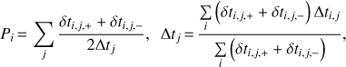
 is a measurement of the median and associated upper and lower errors between a given pair of light curves of a given data set. It corresponds to each single measurement in Fig. 3.
A group of time delay estimates G = [EAB, EAC, EBC] represents the time delays between all pairs j of light curves of the lensed quasar, measured by a given curve shifting technique applied on a given data set. It corresponds to any three points of the same color in each row of Fig. 3.
A series of time delay estimates S = [G1,…Gi,…GN] for i ϵ N is an ensemble of groups of time delay estimates that share the same data set and estimator. A series is typically obtained by varying the estimator parameters and error estimation procedure of a curve-shifting technique. It corresponds to each row of Fig. 3, where N = 5 in this case.
 |
Fig. 3. Time delays estimates and uncertainties (including both the statistical and systematic contributions) between the three pairs of light curves of PG 1115+080. Each column corresponds to a given pair of light curves, indicated in the top-left corner of each panel. Each row corresponds to a series, that is groups of time-delay estimates applied on given data set and curve-shifting technique, the name of which is indicated above the central panel. The estimator parameters corresponding to each group of time-delay estimates are indicated in Table 1. For each two consecutive rows, representing time-delay estimates from the same data set, the symbols correspond to the generative model used when drawing the mock light curves. The shaded region in each panel indicates the combined time-delay estimates for τthresh = 0.5 (see text for details). |
We process each data set the same way. First, we apply the free-knot splines technique, consisting of the free-knot spline estimator applied on the data and mock curves analysis as well as in the mock curves generative model. While exploring various choices of estimator parameters, we choose to use the same parameters when fitting the data, the mocks and in the generative model in order to limit the number of possible configurations to consider. Similarly, we focus on only one type of slow microlensing modeling. For the shorter data sets (WFI and Schechter), we follow Courbin et al. (2018) and use extrinsic splines with a single knot whose position is fixed on the time axis at the middle of the light curves. For the longer data set (Maidanak + Mercator) we use splines with roughly one knot per season, whose position is free to vary during the iterative fitting process, up to a minimal distance of 100 days between the knots. This representation for microlensing leave us with only one estimator parameter to vary, which is the initial knot step η of the spline used to represent the intrinsic variations of the quasar. Eyeballing the fitting of the original data gives us an η to start with, and other η values are explored around this initial guess. As stated earlier, an inappropriate choice of η yields time-delay estimates with larger error bars, thus giving us upper and lower limits for η. The resulting series of time-delay estimates, obtained by using five different η for each data set can be seen in every second row of Fig. 3, with “free-knot splines” in the subtitle.
Second, we apply the regression difference technique consisting of the regression difference estimator used in the data and mock curves analysis, while still using the free-knot spline estimator in the generative model. Here, the choice of the regression difference estimator parameters to fit the data and mock curves is completely independent from the choice of free-knot splines estimator parameters used in the generative model. We first choose five different plausible combinations of regression difference estimator parameters. For simplicity, we decide to use the same generative models as for the free-knot splines technique. Therefore, to each of the five combinations of estimator parameters correspond five possible generative models, each of which influences only the precision of the resulting group of time-delay estimates. For each choice of regression difference estimator parameters, there is one generative model that yields the most precise group of time-delay estimates. In order to assess which group is the most precise, we define the relative precision of a series of time-delay estimates: for each group i in the series, the relative precision reads as
 (1)
where we sum over the j time delay estimates of each group, and where Δtj is the mean of the individual j delays over the i groups of the series. We compute Δtj using the unweighted mean of the Δti,j for simplicity. The results for various choices of estimator parameters are presented in each second row of Fig. 3, with “re-gression difference” mentioned in the subtitle. Each group represents one choice of regression difference estimator parameters, and the symbols indicate which generative model from the corresponding free-knot spline row above has been used.
(1)
where we sum over the j time delay estimates of each group, and where Δtj is the mean of the individual j delays over the i groups of the series. We compute Δtj using the unweighted mean of the Δti,j for simplicity. The results for various choices of estimator parameters are presented in each second row of Fig. 3, with “re-gression difference” mentioned in the subtitle. Each group represents one choice of regression difference estimator parameters, and the symbols indicate which generative model from the corresponding free-knot spline row above has been used.
4. Toward a single group of time-delay estimates
A latent question of PyCS concerns the combination of multiple groups of time-delay estimates obtained with different curve-shifting techniques in order to get a definitive measurement. By construction, a given curve-shifting technique has always one set of estimator parameters for which the best precision is achieved. The expected behavior when varying the estimator parameters is that it impacts mostly the precision while marginally affecting the mean of the measured time delays. Such behavior has always been observed in the previous COSMOGRAIL work and is part of the usual robustness checks, as mentioned earlier. However, the present case is the first time where light curves not obtained with the COSMOGRAIL reduction pipeline are thoroughly analyzed with PyCS. As observed in Fig. 3, the measured mean time delays for the Maidanak + Mercator and Schechter data sets shift with the choice of estimator parameters. Furthermore, the best estimates from two different curve-shifting techniques are not necessarily in excellent agreement. For example, Tewes et al. (2013b) and Bonvin et al. (2017) each present time-delay estimates from both the regression difference and free-knot splines techniques but pick the most precise as the absolute reference, whereas the two techniques agree at the ~one sigma level. In this section, we first combine the groups of time-delay estimates per data set, marginalizing over the possible choice of estimator parameters and curve-shifting techniques weighted by their individual preci-sion. We then discuss the combination of the estimates from the three data sets together and propose two possible results.
4.1. Combining various curve-shifting techniques
In order to combine various groups of time-delay estimates measured on the same data set, we make use of the precision P defined in Eq. (1) but also of the tension between two groups. For two time-delay estimates 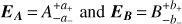 with A > B, the tension in σ units is defined as
 (2)
(2)
For reference, two Gaussian distributions overlapping at their respective 1σ (2σ) points thus have a tension of τ = ~1.4σ (2σ). Therefore, the tension between two groups G1 and G2 is:
 (3)
that is the maximum tension between the time-delay estimates from corresponding pairs of light curves. In order to combine the time-delay estimates together, we proceed in the following way: for each serie of time-delay estimates sharing the same data set and estimator (i.e., each row of Fig. 3), we first pick the most precise group in the series as our reference Gref. In previous COSMOGRAIL publications, this reference would have been our definitive group of time-delay estimates for the consid-ered curve-shifting technique, but in the present case it is rather a starting point that we might or not combine with other groups. To do so, we compute the tension between each group i in the series and the reference group τi,ref. If the tension exceeds a certain threshold τthresh, the corresponding group is flagged. We then pick the most precise of the flagged groups and combine it with the reference group by marginalizing over the respective time-delay estimates probability distributions. This creates a new reference group. We then repeat the procedure above with the remaining groups, until there is none exceeding the tension threshold τthresh. The reference group is then considered as the final group of time-delay estimates for the considered curve-shifting technique and data set. The combined reference estimates are displayed as gray shaded regions in each panel of Fig. 3 for τthresh = 0.5σ. The combined estimates do not follow a Gaussian probability distribution anymore; in such cases, we take as the mean and 1σ error bars the 50th, 16th and 84th percentiles of the distribution, respectively.
(3)
that is the maximum tension between the time-delay estimates from corresponding pairs of light curves. In order to combine the time-delay estimates together, we proceed in the following way: for each serie of time-delay estimates sharing the same data set and estimator (i.e., each row of Fig. 3), we first pick the most precise group in the series as our reference Gref. In previous COSMOGRAIL publications, this reference would have been our definitive group of time-delay estimates for the consid-ered curve-shifting technique, but in the present case it is rather a starting point that we might or not combine with other groups. To do so, we compute the tension between each group i in the series and the reference group τi,ref. If the tension exceeds a certain threshold τthresh, the corresponding group is flagged. We then pick the most precise of the flagged groups and combine it with the reference group by marginalizing over the respective time-delay estimates probability distributions. This creates a new reference group. We then repeat the procedure above with the remaining groups, until there is none exceeding the tension threshold τthresh. The reference group is then considered as the final group of time-delay estimates for the considered curve-shifting technique and data set. The combined reference estimates are displayed as gray shaded regions in each panel of Fig. 3 for τthresh = 0.5σ. The combined estimates do not follow a Gaussian probability distribution anymore; in such cases, we take as the mean and 1σ error bars the 50th, 16th and 84th percentiles of the distribution, respectively.
The results of the two estimators can then be combined together. The free-knot spline technique and regression difference technique, although fundamentally different in their conception cannot be considered as independent estimates when applied to the same data set. Thus, for each data set, the two corresponding sets of time-delay estimates (shaded gray regions in Fig. 3) are considered as equiprobable distributions that are marginalized over (i.e., the probability distributions are summed) to yield a final group of estimates per data set. The combined group of time-delay estimates are presented in Fig. 4, labeled PyCS-WFI, PyCS-Maidanak + Mercator and PyCS-Schechter. They can be compared to time-delay estimates from the literature that use the same data sets. The Schechter data set has been analyzed by Schechter et al. (1997), Barkana (1997) and Pelt et al. (1998). The second monitoring campaign conducted from the Maidanak observatory has yield time-delay estimates measured by Vakulik et al. (2009), Shimanovskaya et al. (2015) and Tsvetkova et al. (2016). On the same data set, Eulaers & Magain (2011) also tried to estimate the time delays but were unsuccessful. The Mercator and WFI monitoring campaigns are for the first time presented and analyzed in this work.
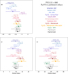 |
Fig. 4. Time delays between the images of PG 1115+080. Each panel compares the already published values from various authors to our own estimates, obtained using PyCS on the same data sets. The new estimates obtained in this work are labeled “PyCS” and are displayed more prominently than the already published estimates. On each panel from top to bottom, the first four estimates are computed using the Schechter data set, the four following estimates are computed using the Maidanak data set. The last two estimates are obtained from two possible combination of our own results on the three data sets, either marginalizing over the probability distributions (PyCS-sum) or multiplying them (PyCS-mult). The quoted mean values and error bars are respectively the 50th, 16th and 84th percentiles of the associated time-delay probability distributions. |
4.2. Combining various data sets
The final groups of time-delay estimates for each data set can be combined into a single, final group. There are two ways of performing such a combination. The conservative approach assumes that there might still be shared systematics between the estimates on the three data sets, due to the use of the same curve-shifting techniques. In such a case, the final combined estimates are obtained by marginalizing over the probability distributions corresponding to each estimate. The second approach assumes that the three sets of time-delay estimates are really independent, meaning that the tension between them (if any) does not results from the curve-shifting techniques used and thus can be combined by multiplying the probability distributions. Asking if the tension hints for unaccounted systematics or can be explained by a statistical fluke can be answered, at least partly, by computing the Bayes Factor F (or evidence ratio) between these two hypothesis. Following Marshall et al. (2006), we find an evidence of FAB = 56, FAC = 25 and FBC = 11 in favor of the statistical fluke hypothesis. Considering only the most apparent case of tension, that is between the BC estimates of WFI and Maidanak + Mercator, we find an evidence of  . Without ruling out the possible presence of systematic errors, a Bayes Factor F > 1 indicates that the considered data sets can be consistently combined into a joint set of time-delay estimates by multiplying the probability distributions.
In Fig. 4, we present the final combined estimates from the three data sets, where PyCS-sum refers to the marginalization over the three data sets and PyCS-mult refers to the joint set of estimates. From the results of Fig. 4 we draw the following conclusions:
Firstly, due to the conservative formalism of PyCS, our own time-delay estimates are in comparison less precise than some of the already published estimates, yet always in reasonable agreement.
Secondly, the WFI data set is in overall the one yielding the most precise time-delay estimates, thanks to the better sampling and photometric precision with respect to the other data sets.
Thirdly, the PyCS – Maidanak set of estimates is obtained by application of the whole analysis pipeline to the Maidanak data only, for the sake of a fair comparison with the literature estimates. It is interesting to note that the addition of the Mercator data to the Maidanak light curves results in a slight decrease of the overall precision. Such an effect can be explained by the absence of well-defined features in the Mercator light curves, or also by microlensing time delay potentially affecting differently the two monitoring campaigns (see Sect. 5). The quality of the Mercator data alone is however not sufficient to precisely measure time delays, and the direct comparison with Maidanak is thus not possible. We decided however to use the joint Maidanak + Mercator data set for our final combination, as the addition of extra years of monitoring usually helps constraining the smooth extrinsic variations modeled by the free-knot spline estimator.
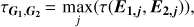
Fourthly, the most stringent tension between the individual PyCS estimates is in the BC delay between Maidanak + Mercator and WFI. Using Eq. (3), we end up with a tension of τ = ~1.9σ. This tension can result from various factors. First, the Maidanak data reduction has been done using a different pipeline that was not under our control, making it hard to exclude a possible systematic bias in the deconvolution. Second, the timescale of the intrinsic variations observed in the Maidanak + Mercator being longer than in WFI, it is more prone to be degenerate with the extrinsic variations. Third, it could also result from a statistical fluke - a two sigma tension has a few percents probability to arise by chance. Last but not least, it could result from microlensing time delay, a systematic error explored in more details in Sect. 5.
Fifthly, the PyCS-sum estimates, although less precise than their PyCS-mult counterpart predict a similar mean value of the time delays. Choosing one or the other for cosmological parameters inference will have an impact on the precision rather than on the accuracy of the results. Being confident that our curve-shifting techniques are sufficiently accurate (Liao et al. 2015; Bonvin et al. 2016), we recommend the use of the joint estimates, that is the PyCS-mult results.
5. Effect of the microlensing time delay
Not to be confused with the traditional microlensing magnification already implemented in PyCS, a microlensing time delay arises when the accretion disk of the quasar is differently magnified by microlenses (stars or other compact objects) located at the position of the lensed images around the lens galaxy. If the accrection disk is modeled following a lamp-post model (Cackett et al. 2007), temperature variations correlate with luminosity variations. When temperature changes at the center of the accretion disk, it propagates along the disk and generates correlated emission on its way, lagged by the time taken for the impulse to propagate from the center to the edges. Thus, the larger the disk, the longer the lag. In the case of no microlensing, these lagged emissions are order(s) of magnitude fainter than the central emission and are contributing similarly from image to image to the integrated emission. However, for a given magnification pattern, different regions of the accretion disk will be differently magnified, and the lagged contributions will contribute differently to the integrated emission from one lensed image to another. In practice, the accretion disk being far too small to be resolved, light curves of images affected by microlensing time delay are seen shifted in time and skewed with respect to the case of no microlensing, resulting in a biased measurement of the time delays.
Tie & Kochanek (2018), who first introduced microlensing time delay, compute its amplitude for the two lensed quasars HE0435-1223 and RXJ1131-1231. They find that the amplitude of the effect depends on the size of the accretion disk of the quasar, its orientation relative to the lens and the amount of microlenses at the position of the lensed images. The microlenses and accretion disk are moving with respect to each other, resulting in a time-variable micromagnification of the disk over many years. However, microlensing time delay does not average out over time. Considering the worst cases (see Table 2 of Tie & Kochanek 2018), the mean bias is on the order of a day. However, for peculiar geometrical configurations this bias can reach several days. Since the relative motion of the accretion disk and microlenses is slow, such a strong bias can affect the light curves for years. Thus, data sets of short duration like the WFI and Schechter data sets are more likely to be strongly affected, if during this short period of time the quasar happens to lie close to a micro caustic. In data sets with longer baseline such as the Maidanak + Mercator data set, it is in principle possible to observe a variation of the measured time delays over the years, although in practice the temporal sampling and photometric precision of our light curves are not sufficient to see an effect season by season.
κ, γ, and κ⋆/κ at each lensed image position from the macro model, based on the modeling in Chen et al. (in prep.).
In the case of PG 1115+080 our three data sets span over two decades, thus if microlensing time delay is at play we should see variations in the measured delays over time. A look at Fig. 3 shows that the measurements are indeed in slight tension, es-pecially the AC and BC time-delays from the WFI and Maidanak + Mercator data sets - the results from the Schechter data sets being not precise enough to conclude in that regard. Attributing the tension solely to microlensing time delay is certainly wrong, yet it indicates that we have no reason not to consider microlensing time delay as a plausible source of systematic. To address it, we follow the same analysis carried out in Tie & Kochanek (2018) but using microlensing characteristics related to PG 1115+080 instead. We present below the main steps of the analysis and redirect the interested reader to Tie & Kochanek (2018) for more details.
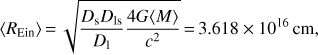
The magnification maps for each lensed image are generated using GPU-D (Vernardos et al. 2014), which is a GPU-accelerated implementation of the inverse ray-shooting technique (Wambsganss et al. 1992). We list the microlensing parameters we used in Table 2. They are based on the lens modeling performed in Chen et al. (in prep.); the lens model is constrained using HST F160W data. The lens total mass is modeled using a NFW profile for the dark matter and a Chameleon profile for the lens light. The latter is converted into baryonic mass through a mass-to-light ratio M/L considered as a free parameter of the model. A prior on M/L is given by the enclosed mass within the Einstein radius, tightly constrained by the visible arc in the lens images. McCully et al. (2017) find, using flexion-shift calculations, that the nearby group plays an important role; it is thus explicitly modeled using a NFW profile, using priors based on the position and velocity dispersion measured by Wilson et al. (2017). To assess the importance of the lens modeling on our microlensing time delay estimates, we also perform our analy-sis using the parameters proposed in Table 1 of Morgan et al. (2008) for a stellar fraction fM/L of 0.7 and 0.8 and find similar results. For each case, we assume a mean mass of the microlenses of ⟨M⟩ = 0.3M⊙ following the Salpeter mass function with a ratio of the upper and lower masses of r = 100 (Kochanek 2004). Our tests show that the choice of mass function influences little the conclusions below. Each map has the size of 20⟨REin⟩ with a 8192-pixel resolution, where
 (4)
which depends on the angular diameter distances from the observer to the lens Dl, the observer to the source Ds, and the lens to the source Dls.
(4)
which depends on the angular diameter distances from the observer to the lens Dl, the observer to the source Ds, and the lens to the source Dls.
To model the quasar accretion disk, we consider a standard thin disk model (Shakura & Sunyaev 1973), which has a radius R0 = 1.629 × 1015 cm in the WFI Rc filter (6517.25 Å) for an Eddington ratio of L/LE = 0.1 and a radiative efficiency of η = 0.1, given an estimated black hole mass of 1.2 × 10⁹M⊙ from Peng et al. (2006). Ignoring the inner edge of the disk, in the simple lamp post model of variability the average microlensing time delay can be derived using Eq. 10 of Tie & Kochanek (2018), reproduced here for convenience:
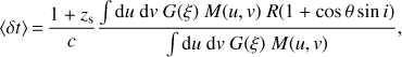 (5)
where G(ξ) is the 1st derivative of the luminosity profile of the disk, ξ = (R/Ro)3/4, M(u, v) is the magnification map projected in the source plane and u, v are the observed coordinates in the lens plane (see Tie & Kochanek 2018, for a detailed explanation of the coordinate system). i and θ represent the inclination and position angle of the disk with respect to the source plane, taken as perpendicular to the observer’s line of sight. For a given geometrical configuration and accretion disk model, we can thus compute the mean excess of microlensing time delay ⟨δt⟩ for a given source position and magnification pattern. By varying the magnification pattern, we can infer a distribution of ⟨δt⟩ for each lensed image.
(5)
where G(ξ) is the 1st derivative of the luminosity profile of the disk, ξ = (R/Ro)3/4, M(u, v) is the magnification map projected in the source plane and u, v are the observed coordinates in the lens plane (see Tie & Kochanek 2018, for a detailed explanation of the coordinate system). i and θ represent the inclination and position angle of the disk with respect to the source plane, taken as perpendicular to the observer’s line of sight. For a given geometrical configuration and accretion disk model, we can thus compute the mean excess of microlensing time delay ⟨δt⟩ for a given source position and magnification pattern. By varying the magnification pattern, we can infer a distribution of ⟨δt⟩ for each lensed image.
In this work, we investigate four disk configurations with inclination i and position angle PA: (i) i = 0°, (ii) i = 60°, PA = 0°, (iii) i = 60°, PA = 45°, and (iv) i = 60°, PA = 90°. The long axis of the tilted disk is perpendicular (parallel) to the caustic structures for PA = 0°(PA = 90°) and corresponds to a face-on disk. We also investigate the effect of decreasing and increasing the source size R0 by a factor of 2. The inferred microlensing time delay distributions, along with their 16th, 50th and 84th percentiles are presented in Fig. 5. We have subtracted the contribution due to the lamp post delay of 5.04(1 + zs)Ro/c. It corresponds to the excess of time delay that would be present even without any microlensing magnification, that cancels out when measuring time delays between two lensed images.
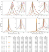 |
Fig. 5. Distributions of the excess of microlensing time delay for the four images of PG 1115+080. The table below the figure reports the 16th, 50th and 84th percentiles of the single image distributions as well as the image pair distributions (see text for details) for the various geometrical configurations explored in this work. |
The mean microlensing time delays from different source configurations follow the trend in Tie & Kochanek (2018). When the disk is perpendicular to the line of sight the microlensing time delay is longer, the disk size R0 drives the amplitude of the effect, and the median excess of microlensing time delay per lensed image is positive, meaning the effect does not fully average out over time. In the worst case scenario explored in this work, the median shift is of half a day, but can reach several days in a few unlucky cases. Contrary to Tie & Kochanek (2018), we report here the percentile values instead of mean and standard deviation of the distributions. The latter are correct approximations only if the distribution follows a Gaussian profile, which is not necessarily the case (see Fig. 5). Depending on the configuration considered, the difference between the mean and 50th percentile can reach a factor of two where the former usually predicts a stronger bias than the latter. It is also interesting to note that the microlensing time delay biases for the C image are much smaller than their A1, A2 and B counterparts, due to the lower fraction of stellar mass κ⋆/κ and lower κ at the C image position.
Propagating the microlensing time delay into our time-delay estimates is done the following way. We first compute the microlensing time delay for image A as the mean of the A1 and A2 individual microlensing delays. This is achieved by convolving the A1 and A2 distributions and rescaling the result by a factor 2. Then, we compute the microlensing time delay affecting each pair of images. To do so, in order to take into account that we observe a difference of microlensing time delays between the lensed images, we mirror one of the distribution with respect to zero before convolving them with each other (in other words, we cross-correlate them). The 50th, 16th and 84th percentiles of the distributions for each pair of images are presented in the table accompanying Fig. 5. To propagate these distributions into the time-delay estimates, one would in turn convolve with the time-delay estimate probability distributions of each data set estimated in Sect. 3.
Ultimately, the question that arises is if microlensing time delay should be added to the time-delay measurements or not. As stated earlier, the 1.9σ tension between the WFI and Maidanak + Mercator data sets, if not uniquely due to microlensing time delay, speaks in favor of it. On the other hand, as mentioned by Tie & Kochanek (2018), not all quasars are well modeled by the thin-disk model, nor by the lamp-post model of variability. Study of accretion disks with microlensing generally finds larger sources sizes that those predicted by the thin-disk model (see e.g., Morgan et al. 2010; Rojas et al. 2014; Jiménez-Vicente et al. 2015), and references therein), and a similar trend emerges from reverberation mapping studies (e.g., Edelson et al. 2015; Lira et al. 2015; Fausnaugh et al. 2016), which motivated the exploration of larger source sizes in this section. The microlensing time delay relies on assumptions about astrophysics that are currently hard to verify experimentally. In conclusion, further work is needed to assess if the effect is still present and with which amplitude when considering, for example, different accretion disk models. In such cases mitigation strategies could be derived, for example by monitoring the quasar in different bands.
We show that the average microlensing time delay values, albeit different from zero are still small enough not to signifi-cantly affect our measured time delays. Presently, we choose not to include the microlensing time delay into our final time delay estimates. All our results are therefore given with error bars that do not include microlensing time delay. However, we present in Sect. 6 how the PyCS-mult estimates change when it is taken into account following the formalism presented in this Section. We also redirect the interested readers to Chen et al. (2018) for a full account of the microlensing time delay at the lens modeling stage.
6. Robustness checks
The results presented in Sect. 4.2 are obtained by marginalizing our curve-shifting techniques over a range of estimators and associated parameters implemented in PyCS. However, not all possible combinations were exhaustively explored and constraining choices were made, for example on how the slow extrinsic variations in the free-knot splines technique were handled. In this section, our goal is to assess whether choosing other options beyond those explored in Sect. 4.2 have a minimal impact on the results. To do so, we use the tension as defined in Eq. (3) to compare the results. In what follows, we refer to the PyCS-mult time-delay estimates obtained in Sect. 4.2 as the fiducial estimates to perform the following checks.
Firstly, we explore various ranges of estimator parameters for the regression difference technique. As highlighted by Steinhardt & Jermyn (2018), it is not possible to know a priori if a Gaussian process regression has converged to its best possible solution, hence the importance of exploring a large range of possible combinations. Limiting ourselves to only five choices of estimator parameter combinations is purely artificial and future improvements of this curve-shifting technique should include a way to go beyond this limitation, for example by using priors with adaptive constraints on the estimator parameters. In the present case, we test the regression difference estimator against extreme values of the estimator parameters, well outside the range used for the fiducial estimates. This results in similar median values but with much larger error bars. The tension stays always below 0.5σ with the fiducial estimates.
Secondly, we vary the microlensing model used in the Maidanak + Mercator data set analysis. Testing against various microlensing models is a good way to assess whether the chosen model is biased by, for example, features of the intrinsic variations being accounted for in the extrinsic variations, or vice-versa. The chosen extrinsic spline initial knot step ηml is increased to 360 and 500 days, either keeping the minimal spacing between the knots at 100 days or increasing it to 180 and 250 days, respectively. In both cases, both the precision and accuracy are similar to the results presented in Sect. 3, with a tension with the fiducial results always below 0.5σ. Assuming there is no microlensing has a much stronger effect, shifting the mean measured time-delays by up to several days. Yet, it is impossible to properly stack the three light curves across all five seasons without allowing for microlensing variability. For this reason, we believe that the results without microlensing should not be used. We avoid decreasing ηml below 100 as in such a regime, intrinsic and extrinsic variations become degenerate and bias the outcome.
Thirdly, we vary the microlensing model used in the Schechter and WFI data set analysis. Similar to the previous point, we want to assess whether the model chosen in the fiducial analysis has any degeneracies between intrinsic and extrinsic features in the light curves. We avoid adding more than one knot to the extrinsic splines since it would make the intrinsic and extrinsic variations degenerate. Instead, we explore an alternative solution by giving more freedom to the central knot, letting its position on the time axis slide up to 50 days closer to both ends of the extrinsic splines. Doing so adds degeneracy between the intrinsic and extrinsic splines, yet remains an interesting robustness test to perform. For the Schechter data set, this alternative microlensing model marginally affects the results, notably because the precision is relatively low. Thus, the maximum tension with the fiducial results is only 0.15σ. For the WFI data set, since the precision is much better the tension between the alternative microlensing and fiducial results goes up to ~0.6σ for the free-knot splines technique with η = 20 and η = 30. Since this exceeds the fiducial threshold τthresh = 0.5σ used for the combination of time-delay estimates in Sect. 3, we perform the whole analysis using this new microlensing model for WFI instead of the fiducial one. Interestingly, the regression difference results computed using the modified microlensing in the generative model for mock light curves remain very close to their fiducial counterparts, with a maximum tension of 0.2σ. Whereas the fiducial regression difference and free-knot splines time-delay estimates on WFI are in excellent agreement, as it can be seen on Fig. 3, this is less true for the modified microlensing results. The fiducial combined WFI results are thus more precise than the modified microlensing ones, the resulting tension between the two being smaller than 0.5σ. The impact on the final joint combination is also barely noticeable, with a maximum tension of ~0.1, and is represented in purple on Fig. 6.
 |
Fig. 6. Results of various robustness checks performed in Sect. 6. The fiducial PyCS-mult time-delay estimates from Fig. 4 are reproduced here as shaded gray regions. |
Fourthly, the sigma threshold value used when combining the sets of time-delay estimates for a given curve-shifting tech-nique and data set, initially chosen at τthresh = 0.5σ, has no motivations other than accounting for the variance of the estimates for a given estimator. We want to make sure that this arbitrary choice has no strong effect on the outcome. We consider here two extreme cases: with τthresh = 1.0σ, the pipeline simply picks the most precise estimates per panel in Fig. 3. With τthresh = 0σ, all estimates of Fig. 3 are combined together. We note that both cases are not very reasonable choices: neither neglecting estimates in tension with the fiducial estimates, nor including known unprecise estimates is correct. However, doing so provides valuable information on the robustness of our final time-delay estimates. The results of this process are presented in Fig. 6. The maximum tension with the fiducial value is of ~0.2 for τthresh = 1σ and ~0.4 for τthresh = 0σ. Both measurements are represented in red and orange on Fig. 6.
Finally, we include the microlensing time delay following the formalism presented in Sect. 5, convolving the microlensing time delay distribution to the time delay measurement error distribution. This is performed individually on the PyCS-Schechter, PyCS-Maidanak + Mercator and PyCS-WFI sets of time-delay estimates. The three estimates are then combined together, hence reducing the random contribution of microlensing time delay. We assume that this can be done without loss of consistency as the three data sets are separated by roughly twice a decade – allegedly enough time for the microlensing configuration to significantly vary. We present in Fig. 6 the result from two configurations: we fix the inclination angle and position at zero, and use source sizes of 1R0 and 2R0. The impact on the final result remains moderate, with a maximum change in accuracy of 3.5% (6%) and a relative decrease of precision, computed through Eq. (1), of 21.1% (71.1%) for a source size of 1R0 (2R0). An alternative approach to include microlensing time delay at the lens modeling stage instead of the measurement stage is presented in Chen et al. (2018) and illustrated with the microlensing time delay results on PG 1115+080 presented in Sect. 5 of this paper.
In this section we tested some specific effects that we thought could affect our results, but as shown in Fig. 6 these remain of low impact. When compared to the fiducial PyCS-mult measurements, the tension always stayed below 0.5σ, thus as-sessing the robustness of our fiducial results.
7. Conclusions
In this paper, we present the light curves of the lensed quasar PG 1115+080 after one season of monitoring at the ESO MPIA 2.2 m telescope. We expand this monitoring campaign with the already published data from various telescopes in the years 1996-1997 (Schechter et al. 1997) as well as data taken between 2004 and 2006 at the Maidanak telescope in Uzbekistan (Tsvetkova et al. 2010). We complement the latter data set with three monitoring seasons at the Mercator telescope taken from 2005 to 2008.
We present individual measurements of the time delays on these data sets using PyCS, a curve-shifting toolbox de-veloped over the years in the COSMOGRAIL collaboration. We notably include in our results estimations of the microlensing time-delay, following the formalism introduced in Tie & Kochanek (2018) as well as a marginalization strategy over the choice of curve-shifting techniques and optimizer parameters in PyCS. Our results are in agreement with previous estimates from the literature. The time-delay estimates obtained using the ESO MPIA 2.2 m telescope monitoring data are the most precise estimates published so far. This demonstrates along with Courbin et al. (2018) how quasi daily observations over a single season at very high signal-to-noise ratio can surpass long-term monitoring carried out less frequently over many seasons.
By combining our measurements on all the data sets, we obtain values for the time delays (without including the microlensing time delay) of 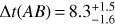 days (18.7% precision),
 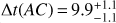 days (11.1%) and
 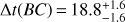 days (8.5%). Our results are robust against how extrinsic intensity variations from microlensing are modeled and how individual set of estimates are combined.
We compute the impact of microlensing time delay for various source parameters. Explicitly accounting for it in the time-delay measurements results in a loss of precision that depend mostly on the chosen size of the accretion disk. We decided not to include it in our final time-delay estimates, as (i) it relies on astrophysical assumptions that are not yet proven to be true (the accretion disk follow a lamp-post model of variability, and is well modeled by a thin-disk model), (ii) there is no clear evidence of microlensing time delay in our data and (iii) a more efficient formalism to handle microlensing time delay at the lens modeling stage is presented in a companion paper (Chen et al. 2018).
Cosmological inference with PG 1115+080 will be carried out in a dedicated paper (Chen et al., in prep.) using AO imaging from the Keck telescope. With two of the three time delays measured around the 10% precision level, PG 1115+080 will be very useful for cosmography when included in a joint analysis of a larger sample of lensed quasars (Treu & Marshall 2016). Ongoing large-sky surveys (e.g., STRIDES, KiDS, CFIS) and future ones (e.g., LSSt, Euclid) will drastically increase the number of known lens systems (e.g., Oguri & Marshall 2010). In such a context, dedicated monitoring telescopes that can yield robust time-delay estimates in a single monitoring season will be crucial.
High-cadence monitoring at the ESO MPIA 2.2 m telescope started in October 2016. Since then, six different lensed quasars have already been monitored for a full season already and three more are currently being monitored on a daily basis. Among these, four targets have been recently discovered and never been monitored before. This work follows the presentation of the time delays of the lensed quasar DES J0408-5354 (Courbin et al. 2018), and represents the second installment of a series of time-delay measurements from high-cadence monitoring soon to be extended.
PyCS can be obtained from http://www.cosmograil.org
Acknowledgments
The authors would like to thank R. Gredel for his help in setting up the program at the ESO MPIA 2.2 m telescope, and the anonymous referee for his or her comments on this work. This work is supported by the Swiss National Fundation. This research made use of Astropy, a community-developed core Python package for Astronomy (Astropy Collaboration et al. 2013, 2018) and the 2D graphics environment Matplotlib (Hunter 2007). K.R. acknowledge support from PhD fellowship FIB-UV 2015/2016 and Becas de Doctorado Nacional CONICYT 2017 and thanks the LSSTC Data Science Fellowship Program, her time as a Fellow has benefited this work. M.T. acknowledges support by the DFG grant Hi 1495/2-1. G. C.-F. C. acknowledges support from the Ministry of Education in Taiwan via Government Scholarship to Study Abroad (GSSA). D. C.-Y. Chao and S. H. Suyu gratefully acknowledge the support from the Max Planck Society through the Max Planck Research Group for S. H. Suyu. T. A. acknowledges support by the Ministry for the Economy, Development, and Tourism’s Programa Inicativa Científica Milenio through grant IC 12009, awarded to The Millennium Institute of Astrophysics (MAS).
References
- Agnello, A. 2017, MNRAS, 471, 2013 [NASA ADS] [CrossRef] [Google Scholar]
- Agnello, A., Lin, H., Buckley-Geer, L., et al. 2017, MNRAS, 472, 4038 [NASA ADS] [CrossRef] [Google Scholar]
- Alam, S., Ata, M., Bailey, S., et al. 2017, MNRAS, 470, 2617 [NASA ADS] [CrossRef] [Google Scholar]
- Astropy Collaboration (Robitaille, T. P., et al.) 2013, A&A, 558, A33 [NASA ADS] [CrossRef] [EDP Sciences] [Google Scholar]
- Astropy Collaboration (Price-Whelan, A. M., et al.) 2018, AJ, 156, 123 [Google Scholar]
- Avestruz, C., Li, N., Lightman, M., Collett, T. E., & Luo, W. 2017, ArXiv e-prints [arXiv:1704.02322] [Google Scholar]
- Barkana, R. 1997, ApJ, 489, 21 [NASA ADS] [CrossRef] [Google Scholar]
- Beaton, R. L., Freedman, W. L., Madore, B. F., et al. 2016, ApJ, 832, 210 [NASA ADS] [CrossRef] [Google Scholar]
- Bennett, C. L., Larson, D., Weiland, J. L., et al. 2013, ApJS, 208, 20 [Google Scholar]
- Bertin, E., & Arnouts, S. 1996, A&AS, 117, 393 [NASA ADS] [CrossRef] [EDP Sciences] [Google Scholar]
- Bonvin, V. F. 2017, PhD Thesis, SB, Lausanne, Switzerland [Google Scholar]
- Bonvin, V., Tewes, M., Courbin, F., et al. 2016, A&A, 585, A88 [NASA ADS] [CrossRef] [EDP Sciences] [Google Scholar]
- Bonvin, V., Courbin, F., Suyu, S. H., et al. 2017, MNRAS, 465, 4914 [NASA ADS] [CrossRef] [Google Scholar]
- Cackett, E. M., Horne, K., & Winkler, H. 2007, MNRAS, 380, 669 [NASA ADS] [CrossRef] [Google Scholar]
- Cantale, N., Courbin, F., Tewes, M., Jablonka, P., & Meylan, G. 2016, A&A, 589, A81 [NASA ADS] [CrossRef] [EDP Sciences] [Google Scholar]
- Cao, S., Zheng, X., Biesiada, M., et al. 2017, A&A, 606, A15 [NASA ADS] [CrossRef] [EDP Sciences] [Google Scholar]
- Chartas, G., Brandt, W. N., Gallagher, S. C., & Proga, D. 2007, AJ, 133, 1849 [NASA ADS] [CrossRef] [Google Scholar]
- Chávez, R., Terlevich, E., Terlevich, R., et al. 2012, MNRAS, 425, L56 [NASA ADS] [CrossRef] [Google Scholar]
- Chen, G. C. F., Fassnacht, C. D., Chan, J. H. H., et al. 2018, ArXiv e-prints [arXiv:1804.09390] [Google Scholar]
- Courbin, F., Bonvin, V., Buckley-Geer, E., et al. 2018, A&A, 609, A71 [NASA ADS] [CrossRef] [EDP Sciences] [Google Scholar]
- DES Collaboration 2017, MNRAS, 480, 3879 [Google Scholar]
- Edelson, R., Gelbord, J. M., Horne, K., et al. 2015, ApJ, 806, 129 [NASA ADS] [CrossRef] [Google Scholar]
- Eulaers, E., & Magain, P. 2011, A&A, 536, A44 [NASA ADS] [CrossRef] [EDP Sciences] [Google Scholar]
- Eulaers, E., Tewes, M., Magain, P., et al. 2013, A&A, 553, A121 [NASA ADS] [CrossRef] [EDP Sciences] [Google Scholar]
- Fausnaugh, M. M., Denney, K. D., Barth, A. J., et al. 2016, ApJ, 821, 56 [NASA ADS] [CrossRef] [Google Scholar]
- Freedman, W. L., Madore, B. F., Scowcroft, V., et al. 2012, ApJ, 758, 24 [NASA ADS] [CrossRef] [Google Scholar]
- Goobar, A., Amanullah, R., Kulkarni, S. R., et al. 2017, Science, 356, 291 [Google Scholar]
- Grillo, C., Rosati, P., Suyu, S. H., et al. 2018, ApJ, 860, 94 [NASA ADS] [CrossRef] [Google Scholar]
- Hege, E. K., Hubbard, E. N., Strittmatter, P. A., & Worden, S. P. 1981, ApJ, 248, L1 [NASA ADS] [CrossRef] [Google Scholar]
- Hunter, J. D. 2007, Comput. Sci. Eng., 9, 90 [Google Scholar]
- Impey, C. D., Falco, E. E., Kochanek, C. S., et al. 1998, ApJ, 509, 551 [NASA ADS] [CrossRef] [Google Scholar]
- Jiménez-Vicente, J., Mediavilla, E., Kochanek, C. S., & Muñoz, J. A. 2015, ApJ, 806, 251 [NASA ADS] [CrossRef] [Google Scholar]
- Joseph, R., Courbin, F., Metcalf, R. B., et al. 2014, A&A, 566, A63 [NASA ADS] [CrossRef] [EDP Sciences] [Google Scholar]
- Kelly, P. L., Rodney, S. A., Treu, T., et al. 2015, Science, 347, 1123 [NASA ADS] [CrossRef] [Google Scholar]
- Kelly, P. L., Rodney, S. A., Treu, T., et al. 2016, ApJ, 819, L8 [Google Scholar]
- Kochanek, C. S. 2004, ApJ, 605, 58 [Google Scholar]
- Kundic, T., Cohen, J. G., Blandford, R. D., & Lubin, L. M. 1997, AJ, 114, 507 [NASA ADS] [CrossRef] [Google Scholar]
- Lanusse, F., Ma, Q., Li, N., et al. 2018, MNRAS, 473, 3895 [NASA ADS] [CrossRef] [Google Scholar]
- Liao, K., Treu, T., Marshall, P., et al. 2015, ApJ, 800, 11 [NASA ADS] [CrossRef] [Google Scholar]
- Lin, H., Buckley-Geer, E., Agnello, A., et al. 2017, ApJ, 838, L15 [NASA ADS] [CrossRef] [Google Scholar]
- Lira, P., Arévalo, P., Uttley, P., McHardy, I. M. M., & Videla, L. 2015, MNRAS, 454, 368 [NASA ADS] [CrossRef] [Google Scholar]
- Magain, P., Courbin, F., & Sohy, S. 1998, ApJ, 494, 472 [NASA ADS] [CrossRef] [Google Scholar]
- Marshall, P., Rajguru, N., & Slosar, A. 2006, Phys. Rev. D, 73, 067302 [NASA ADS] [CrossRef] [Google Scholar]
- McCully, C., Keeton, C. R., Wong, K. C., & Zabludoff, A. I. 2017, ApJ, 836, 141 [NASA ADS] [CrossRef] [Google Scholar]
- Molinari, N., Durand, J., & Sabatier, R. 2004, Comput. Stat. Data Anal., 45, 159 [CrossRef] [Google Scholar]
- More, A., Suyu, S. H., Oguri, M., More, S., & Lee, C.-H. 2017, ApJ, 835, L25 [NASA ADS] [CrossRef] [Google Scholar]
- Morgan, C. W., Kochanek, C. S., Dai, X., Morgan, N. D., & Falco, E. E. 2008, ApJ, 689, 755 [NASA ADS] [CrossRef] [Google Scholar]
- Morgan, C. W., Kochanek, C. S., Morgan, N. D., & Falco, E. E. 2010, ApJ, 712, 1129 [NASA ADS] [CrossRef] [Google Scholar]
- Oguri, M., & Marshall, P. J. 2010, MNRAS, 405, 2579 [NASA ADS] [Google Scholar]
- Patil, A., Huard, D., & Fonnesbeck, C. 2010, J. Stat. Softw., 35, 1 [CrossRef] [EDP Sciences] [Google Scholar]
- Pelt, J., Hjorth, J., Refsdal, S., Schild, R., & Stabell, R. 1998, A&A, 337, 681 [NASA ADS] [Google Scholar]
- Peng, C. Y., Impey, C. D., Rix, H.-W., et al. 2006, ApJ, 649, 616 [Google Scholar]
- Petrillo, C. E., Tortora, C., Chatterjee, S., et al. 2017, MNRAS, 472, 1129 [NASA ADS] [CrossRef] [Google Scholar]
- Planck Collaboration Int. XLVI. 2016, A&A, 596, A107 [NASA ADS] [CrossRef] [EDP Sciences] [Google Scholar]
- Rathna Kumar, S., Tewes, M., Stalin, C. S., et al. 2013, A&A, 557, A44 [NASA ADS] [CrossRef] [EDP Sciences] [Google Scholar]
- Refsdal, S. 1964, MNRAS, 128, 307 [NASA ADS] [CrossRef] [Google Scholar]
- Riess, A. G., Macri, L. M., Hoffmann, S. L., et al. 2016, ApJ, 826, 56 [NASA ADS] [CrossRef] [Google Scholar]
- Riess, A. G., Casertano, S., Yuan, W., et al. 2018, ApJ, 855, 136 [NASA ADS] [CrossRef] [Google Scholar]
- Rodney, S. A., Strolger, L.-G., Kelly, P. L., et al. 2016, ApJ, 820, 50 [NASA ADS] [CrossRef] [Google Scholar]
- Rojas, K., Motta, V., Mediavilla, E., et al. 2014, ApJ, 797, 61 [NASA ADS] [CrossRef] [Google Scholar]
- Rusu, C. E., Fassnacht, C. D., Sluse, D., et al. 2017, MNRAS, 467, 4220 [NASA ADS] [CrossRef] [Google Scholar]
- Schechter, P. L., Bailyn, C. D., Barr, R., et al. 1997, ApJ, 475, L85 [NASA ADS] [CrossRef] [Google Scholar]
- Schechter, P. L., Morgan, N. D., Chehade, B., et al. 2017, AJ, 153, 219 [NASA ADS] [CrossRef] [Google Scholar]
- Shakura, N. I., & Sunyaev, R. A. 1973, A&A, 24, 337 [NASA ADS] [Google Scholar]
- Shimanovskaya, E., Oknyansky, V., & Artamonov, B. 2015, ArXiv e-prints [arxiv:1502.05392] [Google Scholar]
- Sluse, D., Sonnenfeld, A., Rumbaugh, N., et al. 2017, MNRAS, 470, 4838 [NASA ADS] [CrossRef] [Google Scholar]
- Sorce, J. G., Tully, R. B., & Courtois, H. M. 2012, ApJ, 758, L12 [NASA ADS] [CrossRef] [Google Scholar]
- Steinhardt, C. L., & Jermyn, A. S. 2018, PASP, 130, 023001 [NASA ADS] [CrossRef] [Google Scholar]
- Suyu, S. H., Marshall, P. J., Auger, M. W., et al. 2010, ApJ, 711, 201 [NASA ADS] [CrossRef] [Google Scholar]
- Suyu, S. H., Treu, T., Hilbert, S., et al. 2014, ApJ, 788, L35 [NASA ADS] [CrossRef] [Google Scholar]
- Suyu, S. H., Bonvin, V., Courbin, F., et al. 2017, MNRAS, 468, 2590 [Google Scholar]
- Tewes, M., Courbin, F., & Meylan, G. 2013a, A&A, 553, A120 [NASA ADS] [CrossRef] [EDP Sciences] [Google Scholar]
- Tewes, M., Courbin, F., Meylan, G., et al. 2013b, A&A, 556, A22 [NASA ADS] [CrossRef] [EDP Sciences] [Google Scholar]
- Tie, S. S., & Kochanek, C. S. 2018, MNRAS, 473, 80 [NASA ADS] [CrossRef] [Google Scholar]
- Tihhonova, O., Courbin, F., Harvey, D., et al. 2018, MNRAS, 477, 5657 [NASA ADS] [CrossRef] [Google Scholar]
- Tonry, J. L. 1998, AJ, 115, 1 [NASA ADS] [CrossRef] [Google Scholar]
- Treu, T., & Koopmans, L. V. E. 2002, MNRAS, 337, L6 [NASA ADS] [CrossRef] [Google Scholar]
- Treu, T., & Marshall, P. J. 2016, A&ARv, 24, 11 [Google Scholar]
- Tsvetkova, V. S., Vakulik, V. G., Shulga, V. M., et al. 2010, MNRAS, 406, 2764 [NASA ADS] [CrossRef] [Google Scholar]
- Tsvetkova, V. S., Shulga, V. M., & Berdina, L. A. 2016, MNRAS, 461, 3714 [NASA ADS] [CrossRef] [Google Scholar]
- Vakulik, V. G., Shulga, V. M., Schild, R. E., et al. 2009, MNRAS, 400, L90 [NASA ADS] [CrossRef] [Google Scholar]
- Vernardos, G., Fluke, C. J., Bate, N. F., & Croton, D. 2014, ApJS, 211, 16 [NASA ADS] [CrossRef] [Google Scholar]
- Walsh, D., Carswell, R. F., & Weymann, R. J. 1979, Nature, 279, 381 [NASA ADS] [CrossRef] [PubMed] [Google Scholar]
- Wambsganss, J., Witt, H. J., & Schneider, P. 1992, A&A, 258, 591 [NASA ADS] [Google Scholar]
- Weymann, R. J., Latham, D., Roger, J., et al. 1980, Nature, 285, 641 [NASA ADS] [CrossRef] [Google Scholar]
- Wilson, M. L., Zabludoff, A. I., Keeton, C. R., et al. 2017, ApJ, 850, 94 [NASA ADS] [CrossRef] [Google Scholar]
- Wong, K. C., Suyu, S. H., Auger, M. W., et al. 2017, MNRAS, 465, 4895 [NASA ADS] [CrossRef] [Google Scholar]
- Yoo, J., Kochanek, C. S., Falco, E. E., & McLeod, B. A. 2005, ApJ, 626, 51 [NASA ADS] [CrossRef] [Google Scholar]
All Tables
κ, γ, and κ⋆/κ at each lensed image position from the macro model, based on the modeling in Chen et al. (in prep.).
All Figures
|
Fig. 1. Part of the field of view around PG 1115+080, as seen with the ESO MPIA 2.2 m telescope at La Silla Observatory. The field is a stack of 92 exposures with seeing <1.1″ and ellipticity <0.12, for a total of ~8.5 h of exposure. The stars used for the modeling of the PSF are labeled PSF 1 to PSF 6, in red, and the stars used for the exposure to exposure normalization are labeled N1 to N6, in green. The insert shows a single, 330-second exposure of the lens. |
| In the text | |
|
Fig. 2. Light curves for the three data sets used in this work. The B and C components of each data set are shifted in magnitude for visual purposes. The A component corresponds to the integrated flux of the unresolved A1 and A2 quasar images. The WFI and Mercator data are new, while the other observations in the Schechter and Maidanak data were published in Schechter et al. (1997) and Tsvetkova et al. (2010), respectively (see Fig. 2 of both papers). Maidanak and Mercator data overlap during the 2006 season only (see text for details). The inserts show the contribution to the 2006 season from both data sets. |
| In the text | |
|
Fig. 3. Time delays estimates and uncertainties (including both the statistical and systematic contributions) between the three pairs of light curves of PG 1115+080. Each column corresponds to a given pair of light curves, indicated in the top-left corner of each panel. Each row corresponds to a series, that is groups of time-delay estimates applied on given data set and curve-shifting technique, the name of which is indicated above the central panel. The estimator parameters corresponding to each group of time-delay estimates are indicated in Table 1. For each two consecutive rows, representing time-delay estimates from the same data set, the symbols correspond to the generative model used when drawing the mock light curves. The shaded region in each panel indicates the combined time-delay estimates for τthresh = 0.5 (see text for details). |
| In the text | |
|
Fig. 4. Time delays between the images of PG 1115+080. Each panel compares the already published values from various authors to our own estimates, obtained using PyCS on the same data sets. The new estimates obtained in this work are labeled “PyCS” and are displayed more prominently than the already published estimates. On each panel from top to bottom, the first four estimates are computed using the Schechter data set, the four following estimates are computed using the Maidanak data set. The last two estimates are obtained from two possible combination of our own results on the three data sets, either marginalizing over the probability distributions (PyCS-sum) or multiplying them (PyCS-mult). The quoted mean values and error bars are respectively the 50th, 16th and 84th percentiles of the associated time-delay probability distributions. |
| In the text | |
|
Fig. 5. Distributions of the excess of microlensing time delay for the four images of PG 1115+080. The table below the figure reports the 16th, 50th and 84th percentiles of the single image distributions as well as the image pair distributions (see text for details) for the various geometrical configurations explored in this work. |
| In the text | |
|
Fig. 6. Results of various robustness checks performed in Sect. 6. The fiducial PyCS-mult time-delay estimates from Fig. 4 are reproduced here as shaded gray regions. |
| In the text | |
Current usage metrics show cumulative count of Article Views (full-text article views including HTML views, PDF and ePub downloads, according to the available data) and Abstracts Views on Vision4Press platform.
Data correspond to usage on the plateform after 2015. The current usage metrics is available 48-96 hours after online publication and is updated daily on week days.
Initial download of the metrics may take a while.